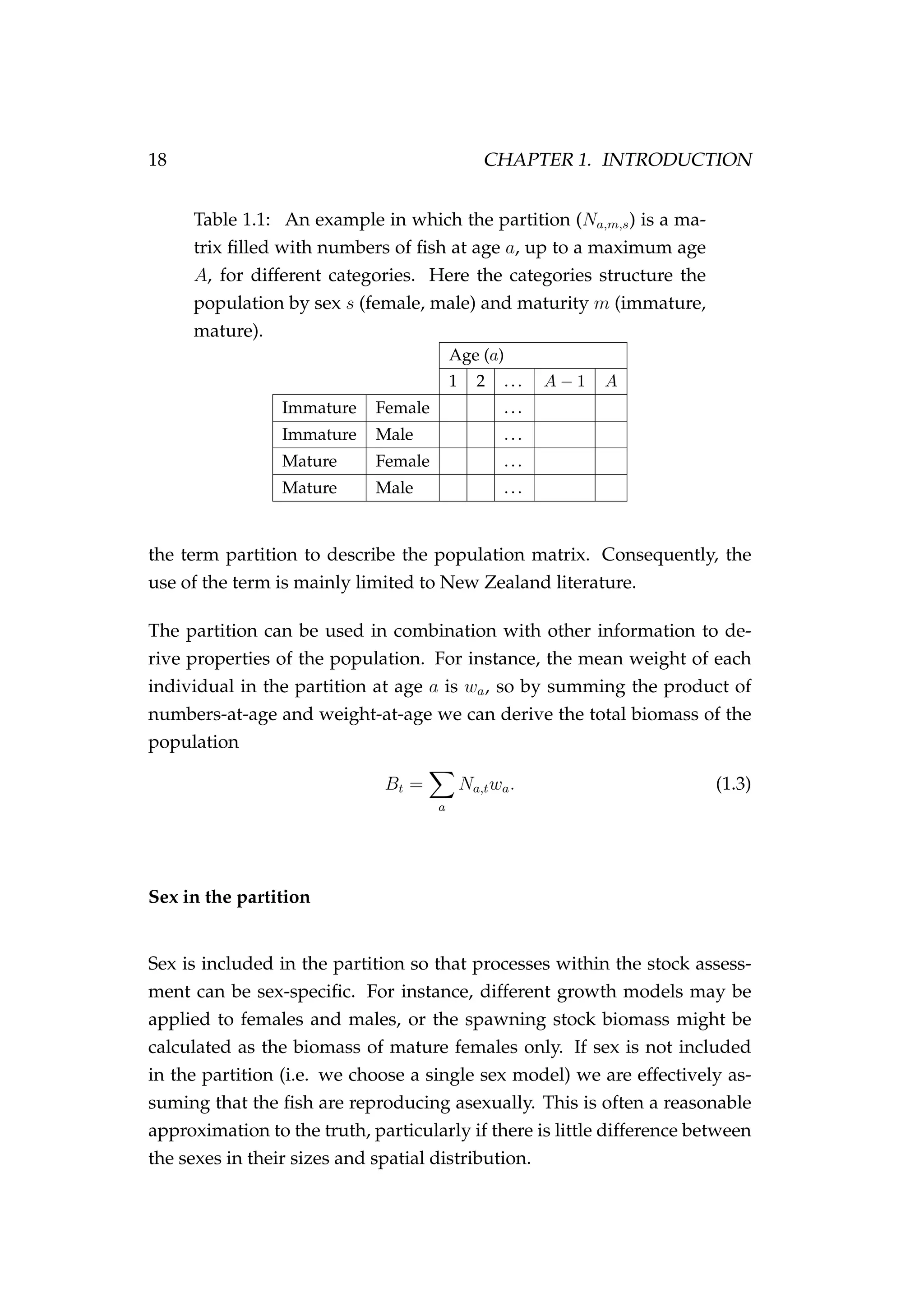
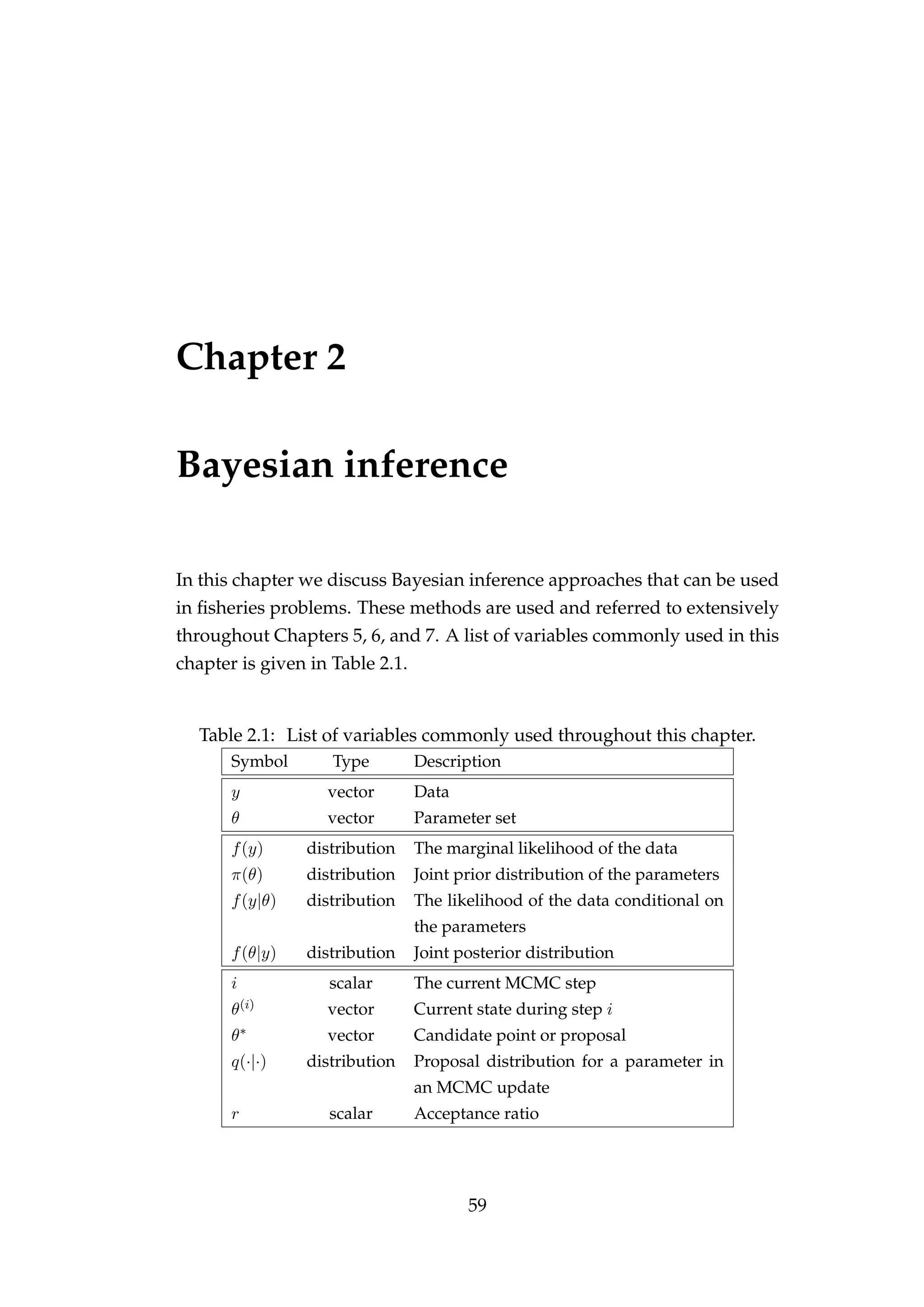
This document is a thesis submitted by D'Arcy N. Webber for the degree of Doctor of Philosophy in Statistics at Victoria University of Wellington in 2015. The thesis develops more realistic fisheries stock assessment models that explicitly model complex processes or quantify uncertainty. It includes the following key components: 1) An agent-based model is developed to better capture individual variability in fish growth, maturation, migration, and mortality for the New Zealand snapper. However, this model has high computational costs. 2) A state-space age-structured model is suggested to better represent uncertainty in stock assessments, but practical application is limited by MCMC mixing issues. 3) A state-space model is presented to estimate

1. Modelling Complexity and
Uncertainty in Fisheries Stock
Assessment
by
D’Arcy N. Webber
A thesis
submitted to the Victoria University of Wellington
in fulfilment of the
requirements for the degree of
Doctor of Philosophy
in Statistics.
Victoria University of Wellington
2015

3. Abstract
Stock assessment models are used to determine the population size of fish
stocks. Although stock assessment models are complex, they still make
simplifying assumptions. Generally, they treat each species separately, in-
clude little, if any, spatial structure, and may not adequately quantify un-
certainty. These assumptions can introduce bias and can lead to incorrect
inferences. This thesis is about more realistic models and their inference.
This realism may be incorporated by explicitly modelling complex pro-
cesses, or by admitting our uncertainty and modelling it correctly.
We develop an agent-based model that can describe fish populations as a
collection of individuals which differ in their growth, maturation, migra-
tion, and mortality. The aim of this model is to better capture the richness
in natural processes that determine fish abundance and subsequent pop-
ulation response to anthropogenic removals. However, this detail comes
at considerable computational cost. A single model run can take many
hours, making inference using standard methods impractical. We apply
this model to New Zealand snapper (Pagurus auratus) in northern New
Zealand.
Next, we developed an age-structured state-space model. We suggest that
this sophisticated model has the potential to better represent uncertainty
in stock assessment. However, it pushes the boundaries of the current
practical limits of computing and we admit that its practical application
remains limited until the MCMC mixing issues that we encountered can
be resolved.
The processes that underpin agent-based models are complex and we may
need to seek new sources of data to inform these types of models. To make
a start here we derive a state-space model to estimate the path taken by in-
dividual fish from the day they are tagged to the day of their recapture.

4. The model uses environmental information collected using pop-up satel-
lite archival tags. We use tag recorded depth and oceanographic temper-
ature to estimate the location at any given time. We apply this model to
Antarctic toothfish (Dissostichus mawsoni) in the Ross Sea.
Finally, to reduce the computational burden of agent-based models we
use Bayesian emulation. This approach replaces the simulation model
with an approximating algorithm called an emulator. The emulator is cal-
ibrated using relatively few runs of the original model. A good emulator
provides a close approximation to the original model and has significant
speed gains. Thus, inferences become tractable.
We have made the first steps towards developing a tractable approach to
fisheries modelling in complex settings through the creation of realistic
models, and their emulation. With further development, Bayesian emula-
tion could result in the increased ability to consider and evaluate innova-
tive methods in fisheries modelling. Future avenues for application and
exploration range from spatial and multi species models, to ecosystem-
based models and beyond.

5. Acknowledgments
Firstly, I would like to thank my supervisors. Richard Arnold, thank you
for the opportunity to work with you in developing this thesis and for
all of your time and ideas. You have helped me develop an invaluable
skill set. Alistair Dunn, thank you for being my go to fisheries science
encyclopedia. Your enthusiasm and wealth of fisheries knowledge has
provided me a great deal of encouragement. And Shirley Pledger, thank
you for all of your guidance and help.
I would like to thank the Ministry for Primary Industries (MPI) and the
National Institute of Water and Atmospheric Research Ltd (NIWA) for
their support of my post-graduate study through the provision of a post-
graduate scholarship in Quantitative Fisheries Science. I would also like to
thank the Victoria University of Wellington for the provision of a Victoria
Doctoral Scholarship.
Thanks Neville Smith and Ben Sharp for your mentorship and advice.
And, thanks to Daniel Fernandez, Roy Costilla, Kath Large, Ash Eaden,
Boyd Anderson, Tom Nation, Matt Dunn, Pamela Mace, Richard Ford,
Jim Thorson, Jim Ianelli, Paul Breen, Paul Starr, Vivian Haaste, Charles
Edwards, Nokome Bentley, Daryl Sykes, Steve Parker, Megan and Christie
Webber, and many more for their help and discussions over the past three
years.
I would also like to thank my reviewers Nokuthaba Sibanda, Andre Punt
and Chris Francis for all of their time and input.
Finally, thank you mum and dad for encouraging me and supporting me
in everything I do and guiding me on my way.
iii

6. iv

7. Contents
Glossary 1
1 Introduction 9
1.1 Research questions . . . . . . . . . . . . . . . . . . . . . . . . 12
1.2 Notation, terminology and layout . . . . . . . . . . . . . . . . 15
1.3 Components of a fisheries model . . . . . . . . . . . . . . . . 17
1.3.1 The partition . . . . . . . . . . . . . . . . . . . . . . . 17
1.3.2 Length and weight at age . . . . . . . . . . . . . . . . 19
1.3.3 Maturation . . . . . . . . . . . . . . . . . . . . . . . . 21
1.3.4 Natural mortality . . . . . . . . . . . . . . . . . . . . . 22
1.3.5 Fishing mortality . . . . . . . . . . . . . . . . . . . . . 24
1.3.6 Spawning stock biomass (SSB) . . . . . . . . . . . . . 24
1.3.7 Recruitment . . . . . . . . . . . . . . . . . . . . . . . . 24
1.3.8 R0 and B0 . . . . . . . . . . . . . . . . . . . . . . . . . 27
1.3.9 Selectivity . . . . . . . . . . . . . . . . . . . . . . . . . 27
1.3.10 Areas, stocks and fisheries . . . . . . . . . . . . . . . . 31
1.3.11 Simulation . . . . . . . . . . . . . . . . . . . . . . . . . 33
1.4 Types of model . . . . . . . . . . . . . . . . . . . . . . . . . . 34
1.4.1 Biomass dynamics models . . . . . . . . . . . . . . . . 35
1.4.2 Age- and length-structured models . . . . . . . . . . 36
1.4.3 Individual-based models . . . . . . . . . . . . . . . . 45
1.5 Data . . . . . . . . . . . . . . . . . . . . . . . . . . . . . . . . . 47
1.5.1 Proportions in the catch-at-age . . . . . . . . . . . . . 49
1.5.2 Abundance indices . . . . . . . . . . . . . . . . . . . . 50
1.6 Fisheries management . . . . . . . . . . . . . . . . . . . . . . 56
1.6.1 Quota Management System (QMS) . . . . . . . . . . . 56
v

8. vi CONTENTS
1.6.2 Total Allowable Commercial Catch (TACC) . . . . . . 56
1.6.3 Annual catch entitlement (ACE) . . . . . . . . . . . . 57
1.6.4 Deemed values (DV) . . . . . . . . . . . . . . . . . . . 58
2 Bayesian inference 59
2.1 Introduction . . . . . . . . . . . . . . . . . . . . . . . . . . . . 60
2.1.1 Bayes’ theorem . . . . . . . . . . . . . . . . . . . . . . 60
2.2 Priors π(θ) . . . . . . . . . . . . . . . . . . . . . . . . . . . . . 61
2.3 Likelihoods f(y|θ) . . . . . . . . . . . . . . . . . . . . . . . . . 62
2.4 Markov chain Monte Carlo (MCMC) . . . . . . . . . . . . . . 62
2.4.1 Metropolis-Hastings (MH) . . . . . . . . . . . . . . . 63
2.4.2 Blockwise MCMC . . . . . . . . . . . . . . . . . . . . 65
2.4.3 Blockwise MH with log-normal proposals . . . . . . 66
2.4.4 Transformations of random variables . . . . . . . . . 67
2.4.5 Proposal variances . . . . . . . . . . . . . . . . . . . . 68
2.4.6 Parallel tempering . . . . . . . . . . . . . . . . . . . . 68
2.5 Bayesian emulation . . . . . . . . . . . . . . . . . . . . . . . . 71
3 Case studies 73
3.1 Antarctic toothfish . . . . . . . . . . . . . . . . . . . . . . . . 73
3.2 Snapper (SNA 1) . . . . . . . . . . . . . . . . . . . . . . . . . 77
3.3 Packhorse rock lobster . . . . . . . . . . . . . . . . . . . . . . 80
4 An agent-based simulation model 89
4.1 Introduction . . . . . . . . . . . . . . . . . . . . . . . . . . . . 89
4.2 The agent . . . . . . . . . . . . . . . . . . . . . . . . . . . . . . 92
4.2.1 Accessing agents . . . . . . . . . . . . . . . . . . . . . 94
4.2.2 Creating agents . . . . . . . . . . . . . . . . . . . . . . 96
4.2.3 Deleting agents . . . . . . . . . . . . . . . . . . . . . . 101
4.2.4 Splitting agents . . . . . . . . . . . . . . . . . . . . . . 102
4.2.5 Moving agents . . . . . . . . . . . . . . . . . . . . . . 103
4.2.6 Merging agents . . . . . . . . . . . . . . . . . . . . . . 105
4.3 Model structure . . . . . . . . . . . . . . . . . . . . . . . . . . 107
4.3.1 Initialisation . . . . . . . . . . . . . . . . . . . . . . . . 107
4.3.2 Applying the fishery . . . . . . . . . . . . . . . . . . . 109
4.4 Processes . . . . . . . . . . . . . . . . . . . . . . . . . . . . . . 109

9. CONTENTS vii
4.4.1 Ageing . . . . . . . . . . . . . . . . . . . . . . . . . . . 110
4.4.2 Growth . . . . . . . . . . . . . . . . . . . . . . . . . . . 110
4.4.3 Maturation . . . . . . . . . . . . . . . . . . . . . . . . 112
4.4.4 Spawning . . . . . . . . . . . . . . . . . . . . . . . . . 112
4.4.5 Recruitment . . . . . . . . . . . . . . . . . . . . . . . . 114
4.4.6 Natural mortality . . . . . . . . . . . . . . . . . . . . . 117
4.4.7 Migration . . . . . . . . . . . . . . . . . . . . . . . . . 117
4.4.8 Fishing mortality . . . . . . . . . . . . . . . . . . . . . 118
4.4.9 Tagging . . . . . . . . . . . . . . . . . . . . . . . . . . 122
4.5 Population calculations . . . . . . . . . . . . . . . . . . . . . . 123
4.6 Technical details . . . . . . . . . . . . . . . . . . . . . . . . . . 123
4.7 Discussion . . . . . . . . . . . . . . . . . . . . . . . . . . . . . 125
5 State-space models 129
5.1 Introduction . . . . . . . . . . . . . . . . . . . . . . . . . . . . 129
5.2 A simple example . . . . . . . . . . . . . . . . . . . . . . . . . 132
5.3 Biomass dynamics state-space models . . . . . . . . . . . . . 137
5.3.1 Inference . . . . . . . . . . . . . . . . . . . . . . . . . . 138
5.3.2 Packhorse rock lobster example . . . . . . . . . . . . . 140
5.4 Age-structured state-space models . . . . . . . . . . . . . . . 163
5.4.1 Inference . . . . . . . . . . . . . . . . . . . . . . . . . . 171
5.4.2 Snapper simulation example . . . . . . . . . . . . . . 179
5.5 Discussion . . . . . . . . . . . . . . . . . . . . . . . . . . . . . 204
6 Pop-up satellite archival tagging 209
6.1 Introduction . . . . . . . . . . . . . . . . . . . . . . . . . . . . 209
6.1.1 Variables recorded by the tags . . . . . . . . . . . . . 214
6.1.2 Environmental data or models (covariates) . . . . . . 214
6.1.3 Projection . . . . . . . . . . . . . . . . . . . . . . . . . 216
6.2 Model development . . . . . . . . . . . . . . . . . . . . . . . 220
6.2.1 The process model . . . . . . . . . . . . . . . . . . . . 220
6.2.2 Observation models . . . . . . . . . . . . . . . . . . . 225
6.2.3 Additional considerations . . . . . . . . . . . . . . . . 229
6.3 Bayesian inference . . . . . . . . . . . . . . . . . . . . . . . . 230
6.3.1 Blockwise Metropolis-Hastings algorithm . . . . . . . 232

10. viii CONTENTS
6.4 Tag 186: the towed tag . . . . . . . . . . . . . . . . . . . . . . 233
6.5 Simulation . . . . . . . . . . . . . . . . . . . . . . . . . . . . . 240
6.6 Tag 121: the tagged fish . . . . . . . . . . . . . . . . . . . . . . 244
6.7 Discussion . . . . . . . . . . . . . . . . . . . . . . . . . . . . . 253
7 Bayesian emulation 259
7.1 Introduction . . . . . . . . . . . . . . . . . . . . . . . . . . . . 259
7.2 Univariate emulators . . . . . . . . . . . . . . . . . . . . . . . 262
7.2.1 A one-dimensional example . . . . . . . . . . . . . . . 273
7.2.2 An example with a stochastic function . . . . . . . . . 275
7.3 Stochasticity in emulators . . . . . . . . . . . . . . . . . . . . 278
7.3.1 A one-dimensional example with stochasticity . . . . 281
7.4 Multivariate emulators . . . . . . . . . . . . . . . . . . . . . . 283
7.5 Inference on an emulator . . . . . . . . . . . . . . . . . . . . . 290
7.6 Univariate emulation of a biomass dynamics model . . . . . 292
7.6.1 The simulator . . . . . . . . . . . . . . . . . . . . . . . 292
7.6.2 The emulator . . . . . . . . . . . . . . . . . . . . . . . 294
7.6.3 Inference . . . . . . . . . . . . . . . . . . . . . . . . . . 296
7.7 Multivariate emulation of a stochastic agent-based model . . 298
7.7.1 The simulator . . . . . . . . . . . . . . . . . . . . . . . 298
7.7.2 The emulator . . . . . . . . . . . . . . . . . . . . . . . 302
7.7.3 Inference . . . . . . . . . . . . . . . . . . . . . . . . . . 305
7.8 Discussion . . . . . . . . . . . . . . . . . . . . . . . . . . . . . 310
8 Conclusions and future research 317
Appendix A The log-normal distribution 323
A.1 Probability density function (PDF) . . . . . . . . . . . . . . . 323
A.2 Expectation . . . . . . . . . . . . . . . . . . . . . . . . . . . . 323
A.3 Using a log-normal proposal distribution . . . . . . . . . . . 325
Appendix B Age-structured state-space models 327
B.1 Equilibrium numbers at age proof . . . . . . . . . . . . . . . 327
B.2 Model validation . . . . . . . . . . . . . . . . . . . . . . . . . 328
B.3 Model fit (fixed process error) . . . . . . . . . . . . . . . . . . 328
B.4 Model fit (releasing σ2
R) . . . . . . . . . . . . . . . . . . . . . . 336

11. CONTENTS ix
Appendix C Pop-up satellite archival tagging 341
C.1 GPS coordinates for tag 186 . . . . . . . . . . . . . . . . . . . 341
C.2 MCMC diagnostics . . . . . . . . . . . . . . . . . . . . . . . . 341
Appendix D Agent-based model of snapper (SNA 1) 351
D.1 ABM input file . . . . . . . . . . . . . . . . . . . . . . . . . . . 351
D.2 Plots of ABM output . . . . . . . . . . . . . . . . . . . . . . . 355
References 365

12. x CONTENTS

13. Glossary
Byear is the estimated or predicted biomass in the named year (usually a
mid-year biomass). 76, 80
abundance a measure of fish density, numbers or total biomass. i, 1, 7, 17,
36, 37, 51, 54, 55, 75, 132, 138, 171
abundance index a quantitative but relative (i.e. uncalibrated) measure
of fish density, numbers or total biomass. An abundance index can be
specific to an area or to a segment of the stock (e.g. mature fish), or it can
refer to abundance stock-wide. 2, 9, 47, 50, 51
ACE Annual Catch Entitlement. 57, 58
age-frequency (Pa) the proportions of fish of different ages in the stock,
or in the catch taken by either the commercial fishery or research fishing.
This is often estimated based on a sample. Sometimes called an age com-
position. 49, 75
age-length key (M
key
a, ) the proportion of fish of each age in each length-
group in a catch (or stock) of fish. 49, 50
biomass (Bt) refers to the size of the stock in units of weight. Often,
biomass refers to only one part of the stock (e.g. spawning stock biomass,
recruited biomass, or vulnerable biomass the later two of which are essen-
tially equivalent). 1, 2, 6, 7, 9, 17, 33–36, 50, 51, 54, 123, 129, 137, 139
bycatch refers to fish species, or size classes of those species, caught unin-
tentionally in association with key target species. 81
C++ is a general-purpose programming language. It has object-oriented
programming features, while also providing the facilities for low-level
memory manipulation. 93, 123, 125
1

14. 2 Glossary
carrying capacity (K) is the average stock size expected in the absence
of fishing. Even without fishing the stock size varies through time in re-
sponse to stochastic environmental conditions. 7, 33, 35, 137–139, 296
catch (Ct) is the total weight (or sometimes numbers) of fish caught by
fishing operations. Sometimes referred to as landings. The catch can be
split by age Ca,t or by size C ,t. i, 1–4, 9, 24, 33, 35, 37, 42, 44, 47, 49–51, 54,
58, 75, 83, 84, 86, 118, 122, 130, 132, 138, 139, 141, 148, 163, 171, 172, 179,
180, 293, 296, 300, 305
catch-per-unit-effort (CPUE) (It) is the quantity of fish caught with one
standard unit of fishing effort; e.g. the number of fish taken per 1000 hooks
per day or the weight of fish taken per hour of trawling. CPUE is often
assumed to be an abundance index. 9, 36, 47, 50–52, 54, 86, 87, 130, 137,
138, 171, 296, 305
catchability (q) is the proportion of fish that are caught by a defined unit
of fishing effort. It is a constant relating an abundance index to the true
biomass (the abundance index is approximately equal to the true biomass
multiplied by the catchability). 36, 51, 54, 90, 122, 137, 139, 141, 172, 181,
293, 296, 305
CCAMLR Convention for the Conservation of Antarctic Marine Living
Resources. 73–76
CELR Catch Effort Landing Return. 86
coefficient of variation (CV) is a standardised measure of dispersion of a
probability distribution or frequency distribution. It is defined as the ratio
of the standard deviation to the mean. 99, 166
cohort refers to those individuals of a stock born in the same spawning
season. For annual spawners, a years recruitment of new individuals to a
stock is a single cohort or year-class. 2, 17, 34, 36, 37, 91, 92, 125
CRA red rock lobster (Jasus edwardsii), commonly known as crayfish. 80–
82, 86
CSIRO Commonwealth Scientific and Industrial Research Organisation.
215
demersal species live and feed on or near the bottom of seas or lakes (the
demersal zone). 255
deterministic a deterministic system is a system in which no randomness

15. Glossary 3
is involved in the development of future states of the system. A deter-
ministic model will thus always produce the same output from a given
starting condition or initial state. 6, 19, 94, 109, 110, 171, 240, 259
DV Deemed Value. 58
EEZ Exclusive Economic Zone. 56, 83
equilibrium A theoretical condition that arises when the fishing mortal-
ity, exploitation patterns and other fishery or stock characteristics (growth,
natural mortality, recruitment) are balanced and sustainable and thus do
not change from year to year. 33, 35, 107
exploitation rate (U) is the proportion of the recruited or vulnerable
biomass that is caught during a certain period, usually a fishing year. 24,
40, 42, 44, 118, 123, 171
fishing mortality (F) is the fishing mortality rate. 3, 11, 24, 42–44, 54, 101,
138
fishing year (t) For most stocks in New Zealand, the fishing year runs
from 1 October in one year to 30 September in the next. The second year is
usually used as shorthand for the split years. For example, 2005 refers to
the fishing year running from 1 October 2004 to 30 September 2005. 3, 52,
57, 214, 244
FishServe FishServe is the trading name of a privately owned company
called Commercial Fisheries Services (CFS). CFS is a wholly owned sub-
sidiary of Seafood New Zealand (SNZ). FishServe provides administrative
services to the New Zealand commercial fishing industry to support the
1996 Fisheries Act. 57
FMA Fisheries Management Area. 56
Fortran (previously FORTRAN, derived from Formula Translating Sys-
tem) is a general-purpose, imperative programming language that is es-
pecially suited to numeric computation and scientific computing. 256
Git is a distributed revision control system for distributed, non-linear
workflows. Git was initially designed and developed by Linus Torvalds
for Linux kernel development in 2005, and has since become the most
widely adopted version control system for software development. 3, 4
GitHub is a web-based Git repository hosting service, which offers all of

16. 4 Glossary
the distributed revision control and source code management functional-
ity of Git as well as adding its own features (https://github.com/).
16
GPS global positioning system. 214, 215, 217, 218, 234–236, 239, 253
heterogeneous composed of parts of different kinds; having widely dis-
similar elements or constituents; not homogeneous. 4, 10, 13, 92, 125, 317
homogeneous composed of parts or elements that are all of the same kind;
not heterogeneous. 4, 11, 56, 75
ITQ Individual Transferable Quota. 57
Julia is a high-level, dynamic programming language for technical com-
puting (http://julialang.org/). 206, 220, 254, 256, 322
length-frequency (Q ) the proportions of fish of different lengths in the
stock, or in the catch, taken by either the commercial fishery or research
fishing. This is often estimated based on a sample. Sometimes called a
length or size composition. 49, 50, 75, 86
Linux is a Unix-like computer operating system assembled under the
model of free and open-source software development and distribution.
The defining component of Linux is the Linux kernel, an operating system
kernel first released on 5 October 1991 by Linus Torvalds. 3, 123
maturity refers to the ability of fish to reproduce. i, 1, 10, 17, 18, 21–24, 40,
89, 90, 92, 93, 96, 112, 171, 172
MCMC Markov chain Monte Carlo. 13, 59, 62–69, 133–137, 139, 140, 142,
143, 145–149, 151, 155, 157, 158, 160, 162, 163, 174, 177, 180, 182–184, 191–
194, 201–203, 205, 220, 227, 232, 233, 235, 237, 240, 241, 244, 246, 247, 253,
254, 256, 259, 299, 309, 310, 325, 327–340
MHR Monthly Harvest Return. 84, 86
MLS minimum legal size. 79, 83, 86
MPI Ministry for Primary Industries. iii, 56, 58, 83, 86
multithreading is a widespread programming and execution model that
allows multiple threads to exist within the context of a single process.
These threads share the process’s resources, but are able to execute in-
dependently. Multithreading can be applied to a single process to enable
parallel execution on a multiprocessing system. 95, 125, 220

17. Glossary 5
natural mortality (M) is the natural mortality rate caused by predation
and other natural processes and is normally calculated on an annual basis.
3, 22–24, 33, 37, 39, 40, 42–44, 46–48, 90, 93, 96, 101, 107, 108, 117, 130, 138,
163, 171, 172
NIWA National Institute of Water and Atmospheric Research Ltd. iii, 17,
79, 213
otolith one of the small bones in the internal ear of fish that can sometimes
be used to determine their age. This involves counting rings in the bone
that correspond to annual growing seasons. 19, 49
PHC packhorse rock lobster (Sagmariasus verreauxi). 81, 83, 86, 87, 129, 140
photic zone or sunlight zone, extends from the surface down to a depth
where light intensity falls to one percent of that at the surface. Accord-
ingly, this depth depends on the extent of light attenuation in the water
column. Typical depths vary from only a few centimetres in highly turbid
eutrophic lakes, to around 200m in the open ocean. 212
pointer in computer science, a pointer is a programming language object,
whose value refers to (or “points to”) another value stored elsewhere in
the computer memory using its address. A pointer references a location in
memory. Obtaining the value stored at that location is known as derefer-
encing the pointer. As an analogy, a page number in a book’s index could
be considered a pointer to the corresponding page; dereferencing such a
pointer would be done by flipping to the page with the given page num-
ber. 94–96, 101, 103
PSAT pop-up satellite archival tag. 75, 76, 209, 212–214, 216, 253, 256
QMA Quota Management Area. 52, 56, 81
QMS Quota Management System. 56–58, 79, 83
R is high-level software environment for statistical computing and graph-
ics (http://www.r-project.org/). 62, 220
recruitment (Rt) is the addition of new individuals to the fished compo-
nent of a stock. This is determined by the size and age at which fish are
first able to be caught. 2, 3, 24–27, 33, 35, 37, 42, 47, 90, 107, 114, 115
selectivity (Sx) a curve describing the relative vulnerability of fish of dif-
ferent ages (x = a), lengths (x = ) or weights (x = w) to the fishing gear

18. 6 Glossary
used. 24, 27, 29–31, 33, 37, 40, 47, 90, 118, 122, 130, 163, 171
selectivity ogive (Sx) see selectivity. 122
SNA snapper (Pagurus auratus). 77, 79, 80, 129, 180
spawning stock biomass (SSBt) refers to the portion of a stocks biomass
that is mature. 1, 18, 24, 25, 27, 32, 37, 38, 40, 42, 92, 107, 112, 114, 115, 123,
124
standard deviation (σ) (SD) is a measure that is used to quantify the
amount of variation or dispersion of a set of data values. 2, 15, 50, 90,
133, 140–142, 148–155, 157–159, 210, 211, 215, 216, 218, 221, 222, 225, 226,
230–232, 234–237, 240, 241, 245–247, 254, 255, 274–277, 293
stochastic a purely stochastic system is one whose state is randomly de-
termined, having a random probability distribution or pattern that may be
analysed statistically but may not be predicted precisely. In this regard, it
can be classified as non-deterministic. 109, 111, 137, 259, 278, 281
stock a biological stock is a population of a given species that forms a
reproductive unit and spawns little if at all with other units. However,
there are many uncertainties in defining spatial and temporal geographi-
cal boundaries for such biological units that are compatible with current
data collection systems. For this reason, the term stock is often synony-
mous with an assessment/management unit, even if there is migration or
mixing of some components of the assessment/management unit between
areas. i, 1–7, 9, 11, 17, 24, 25, 27, 31–33, 35–38, 47, 50, 51, 56–58, 75–77, 80,
86, 90, 99, 100, 107, 124, 129, 163, 209, 300, 319
stock assessment is the application of statistical and mathematical tools
to relevant data to obtain a quantitative understanding of the status of a
stock relative to defined benchmarks or reference points (e.g. BMSY, FMSY).
i, 9–14, 18–21, 23, 27, 31, 35, 36, 47, 51, 54, 55, 60, 75, 76, 86, 87, 91, 92, 125,
127, 129, 163, 166, 171, 204, 206, 209, 212, 319
TAC Total Allowable Catch. 57
TACC Total Allowable Commercial Catch. 57, 58, 79, 83, 84
TOT Antarctic toothfish (Dissostichus mawsoni). 73, 209
variance (σ2
) variance measures how far a set of numbers is spread out.
15, 26, 31, 47, 61, 139, 142, 148, 154, 155, 157–159, 165, 168–172, 181, 200,
204, 205, 207, 229, 254, 264, 266, 270, 275, 276, 278, 279, 281, 286, 293, 296,

19. Glossary 7
305, 323, 325
virgin biomass (B0) is the theoretical carrying capacity of the spawning,
recruited or vulnerable biomass of a fish stock. In some cases, it refers to
the average biomass of the stock in the years before fishing started. More
generally, it is the average biomass that theoretically would have occurred
if the stock had never been fished. 25, 27, 76, 114, 123
vulnerable biomass (Vt) refers to the portion of a stocks biomass that
is available to the fishery. Also called exploitable biomass or recruited
biomass. 1, 3, 7, 38, 40, 42, 50, 54, 118, 122–124, 163
WGS84 The World Geodetic System of 1984. 216
year class (cohort) refers to fish in a stock that were born in the same year.
Occasionally, a stock produces a very small or very large year class which
can be pivotal in determining stock abundance in later years. 2, 25, 26, 115

20. 8 Glossary

21. Chapter 1
Introduction
Commercial and ecological management of fisheries requires good esti-
mates of stock sizes: that is, the number of individuals or total biomass
in a fish population of a particular species. The current practice in fish-
eries science is to fit a model, on which stock assessment is based, to data.
The results of these models are then passed on to managers to make de-
cisions about allowable catches, taking into account the outcome and un-
certainty of the model (Harwood & Stokes 2003, Hilborn 2003). Modern
stock assessment models are generally large statistical models and often
make use of all available data. These data include: estimates of total re-
movals (catch); fishery independent surveys; indices of abundance such as
catch per unit effort (CPUE); age and length structure of the catch and/or
population; biological parameters; and in special cases may incorporate
tagging data, environmental covariates, genetic information, and/or eco-
nomic data (Anderson 1977).
Despite their complexity, stock assessment models are still simplified ver-
sions of reality. They are simplistic in that they tend to lump fish together
into broad categories or groups (i.e. all fish within a year are lumped to-
gether in biomass dynamics models or all fish of the same age in the same
year are lumped together in age-structured models) and treat all of the
individuals within each of these groups in the same way. For example,
stock assessment models might lump populations together for manage-
ment convenience, and/or they may treat fish from broad spatial areas
9

22. 10 CHAPTER 1. INTRODUCTION
together in the same way. We expand on each of these concepts in the
following paragraphs.
Organisms in the marine environment are likely to exhibit variation in
behavioral or phenotypic traits among individuals (e.g. growth rates,
condition, maturity), and this variation may be persistent (e.g. particu-
lar individuals growing faster/slower throughout their entire lifetime) or
transient (e.g. particular individuals growing faster in one year than in
another year). Many recent studies of captive or wild populations have
demonstrated examples of such persistent differences, termed differences
in “personality” (Wolf & Weissing 2012). For example, persistent differ-
ences in activity level or tolerance of predation risk (i.e. a tendency to
forage in high vs. low-quality habitat) will likely lead to persistent differ-
ences in growth rates among individuals. Subsequently, persistent differ-
ences in growth rate, combined with size-selective harvest targeting larger
individuals, can result in older individuals being composed primarily of
slow-growing individuals (termed “Rosa Lees Phenomenon”), and has
been demonstrated to occur in small-lake mesocosm experiments (Biro &
Post 2008).
Individuals are also likely to experience transient variation in natural pro-
cesses. Such transient variation could be caused by many different pro-
cesses including movement between warmer/colder ambient tempera-
tures (and hence transient variation in metabolic rates), periodic access to
improved feeding (Armstrong & Schindler 2011), and year-specific deci-
sions regarding the allocation of resources between growth and reproduc-
tion (Jorgensen & Fiksen 2006). Several recent studies have also demon-
strated transient differences in behavioural or phenotypic traits among in-
dividuals (Shelton et al. 2013, Webber & Thorson 2015). Failure to account
for persistent or transient differences in growth rate can lead to biased es-
timation of average growth rates in populations and subsequently lead to
biases in stock assessment.
Population variability, (such as average growth, maturity, etc) can also
be important and Punt (2003b) demonstrates that spatial heterogeneity in
growth can affect stock assessment outcomes and that better outcomes

23. 11
can be realised by doing assessments at the population level rather than
pooling data across different populations and carrying out assessments on
these pooled data.
Despite these known risks, stock assessment models are typically devel-
oped for broad scale management and fish stocks are often assumed to
be discrete and spatially homogeneous (Stephenson 1999). As a result,
many stock assessment models have little or no incorporation of spatial
variation or dependence and often stocks are managed over areas that are
either smaller or larger than the true (biological) stock area. In reality,
fish populations are far from spatially homogeneous (Ralston & O’Farrell
2008). Yet the implementation of spatial structure in stock assessment
models has been slow. Although the importance of accounting for spa-
tial population structure in stock assessment is acknowledged (Cadrin &
Secor 2009), the impacts of simplifying assumptions are not yet fully un-
derstood. Spatial complexity can take many forms, including: gradients of
fishing mortality occurring across stock or management boundaries (Siler
et al. 1986); or fishing mortality can be much higher in spatially aggre-
gated clumps (Prince 2003); and high fishing mortality in small areas can
lead to localised depletion while the stock as a whole may still appear
healthy. Furthermore, additional layers of complexity may be introduced
when marine protected areas (MPAs) are declared within stock boundaries
by displacing fishing effort.
Further complications arise when we consider that often stock assessment
models further simplify fisheries systems by largely ignoring ecosystem
interactions (e.g. other species or environmental influences).
Finally, stock assessment models should provide estimates with as little
bias as possible, have the ability to deal with uncertainty, and the uncer-
tainty in the data should be properly reflected in the estimates produced
by the models. Although quantifying uncertainty is an important topic
in fisheries, current stock assessment models tend to underestimate the
true uncertainty (Magnusson et al. 2013). This can produce biased re-
sults (Mormede, Dunn & Hanchet 2013) which can lead to incorrect in-
ferences (Hoshino et al. 2014). One of the key problems we are faced

24. 12 CHAPTER 1. INTRODUCTION
with is separability of the different variance components (i.e. observation
and process error). This is a well known problem in these types of mod-
els (Hilborn & Mangel 1997, Schnute 1987). Therefore, models are needed
that better represent the uncertainty that is characteristic of fisheries data.
Stock assessment models that do take into account some of these addi-
tional complexities in fish populations are at the forefront of fisheries mod-
elling, but often push the limits of available data and computing power.
However, before models like this are adopted, and resources are allocated
to collecting the data to “feed” them, we must first consider whether or not
our current models do an adequate job. If not, then we open a Pandora’s
box of questions. When does modelling space begin to matter? How can
we include individual level variability in our models? Do environmental
drivers influence populations more than fishing? Where do we stop?
This thesis is about more realistic models and their inference. We identify
four specific research questions below.
1.1 Research questions
The primary research questions considered in this thesis include:
1. Can we develop models to better capture complexity, including
spatial richness and individual variability, inherent in real fish
populations?
2. Can we do better at modelling uncertainty in “classic” stock as-
sessment?
3. More complex stock assessments will require richer sources of
data, particularly spatially explicit data. Can we extract some of
these data from pop-up satellite archival tag technology?
4. Bayesian inference of fisheries models can be slow and we are
looking to make them more complex and thus slower. Can we
speed up the Bayesian inference of complex fisheries models?

25. 1.1. RESEARCH QUESTIONS 13
While the focus of this thesis is stock assessment, no formal stock assess-
ments are done. All applications of the models developed use simulated
data, based loosely on case study species (except for Chapter 6). The main
contributions in this thesis are found in Chapters 4, 5, 6 and 7. The pre-
ceding chapters provide the background material required for these core
chapters.
The remainder of this chapter introduces stock assessment modelling and
provides a literature review on stock assessment. Section 1.2 introduces
some of the mathematical terminology used throughout the thesis. Sec-
tion 1.3 gives an overview of the components of a stock assessment model.
Section 1.4 discusses some of the model structures that have been devel-
oped to date. Section 1.5 introduces the types of data used to inform the
parameters of stock assessment models. Finally, Section 1.6 briefly intro-
duces the fisheries management system in New Zealand.
Chapter 2 introduces Bayesian inference methods including Metropolis-
Hastings Markov chain Monte Carlo (MCMC), parallel tempering and
Bayesian emulation. These methods are discussed and used extensively
throughout the rest of the thesis.
Chapter 3 introduces three case study species: Antarctic toothfish (Dis-
sostichus mawsoni), snapper (Pagurus auratus) and packhorse rock lobster
(Sagmariasus verreauxi). Both snapper and packhorse rock lobster are used
in later chapters to develop simulation models. The data from a pop-up
satellite archival tag (PSAT) that was attached to an Antarctic toothfish for
a year is used to develop a novel state-space model in Chapter 6.
Chapter 4 describes a spatially explicit multi-generational agent-
structured fish simulation model that allows flexibility in specifying pop-
ulation and spatial dynamics. The model has the potential to consider
individual variability, individual movement, and spatial heterogeneity in
the environment. The aim was to construct a model that is sufficiently
rich that it can be used to simulate complete, realistic fish populations.
The simulated data can be used to test stock assessment methodologies -
which are usually based on samples from the population, and incomplete
data. The capability of the model is illustrated through an application to

26. 14 CHAPTER 1. INTRODUCTION
snapper.
Chapter 5 introduces state-space models and their inference. The chapter
begins by introducing state-space models using biomass dynamics mod-
els as an example (see Section 1.4.1, page 35). While these are nothing
new, the age-structured state-space model described next is novel. This
age-structured state-space model includes process error in the mid-year
numbers at age in the modelled population, attempting to better capture
model uncertainty in stock assessment. The posterior distribution of this
model is developed, and sophisticated MCMC methods are implemented
in an attempt to sample from the posterior distribution. However, efficient
sampling proved difficult for this model.
In Chapter 6, a novel state-space model for estimating the path taken by
individual fish is developed making use of PSAT data. The difference be-
tween this model and other models is that this model is conditional on the
start and end location. In contrast, other models may not fix the end point
(often called diffusion models or random walks). Our model also attempts
to use depth and temperature, rather than the standard light and temper-
ature, to estimate the location of the fish at any given time. The model is
applied to data collected from a PSAT attached to an Antarctic toothfish in
the Ross Sea region. Although this application was not entirely successful,
the model shows promise for future applications to this and other species.
Chapter 7 explores Bayesian emulation in detail and applies the method in
a series of examples - starting with simple deterministic univariate exam-
ples, up to stochastic fisheries models nested within a state-space frame-
work.
Finally, the thesis concludes with a discussion in Chapter 8.
We provide a list of original contributions to fisheries science and statistics
that this thesis makes here to aid the reader as they progress through the
document:
• A comprehensive agent-based simulation model (Chapter 4)
• Further development of age-structured state-space models (Chap-
ter 5)

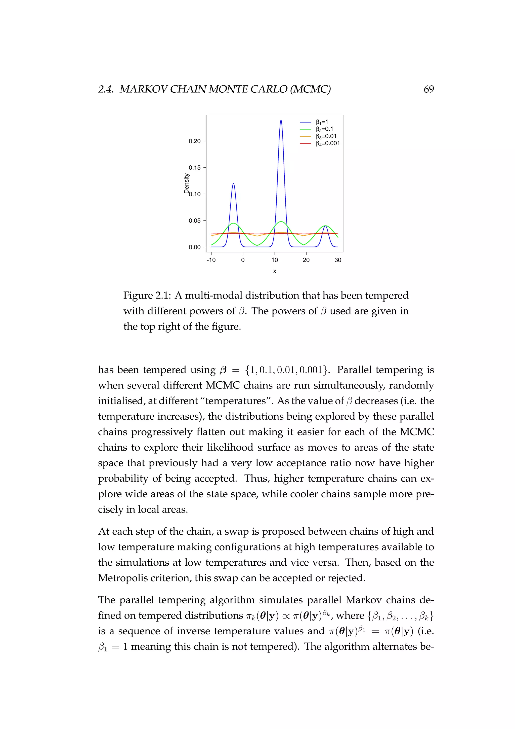
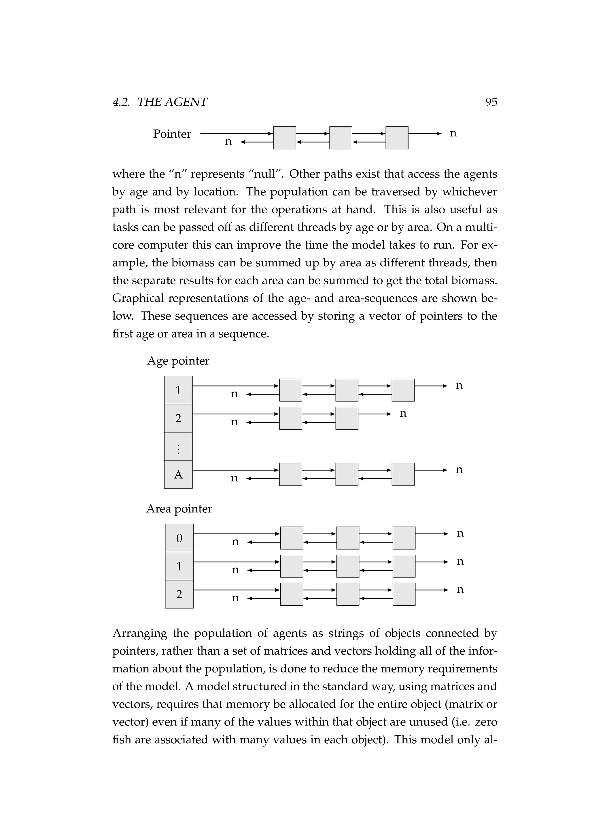
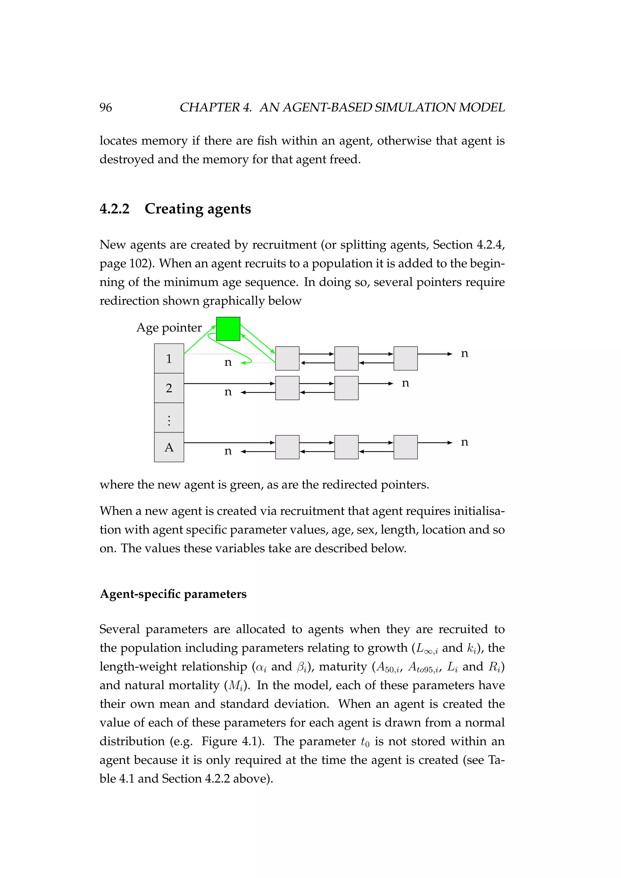
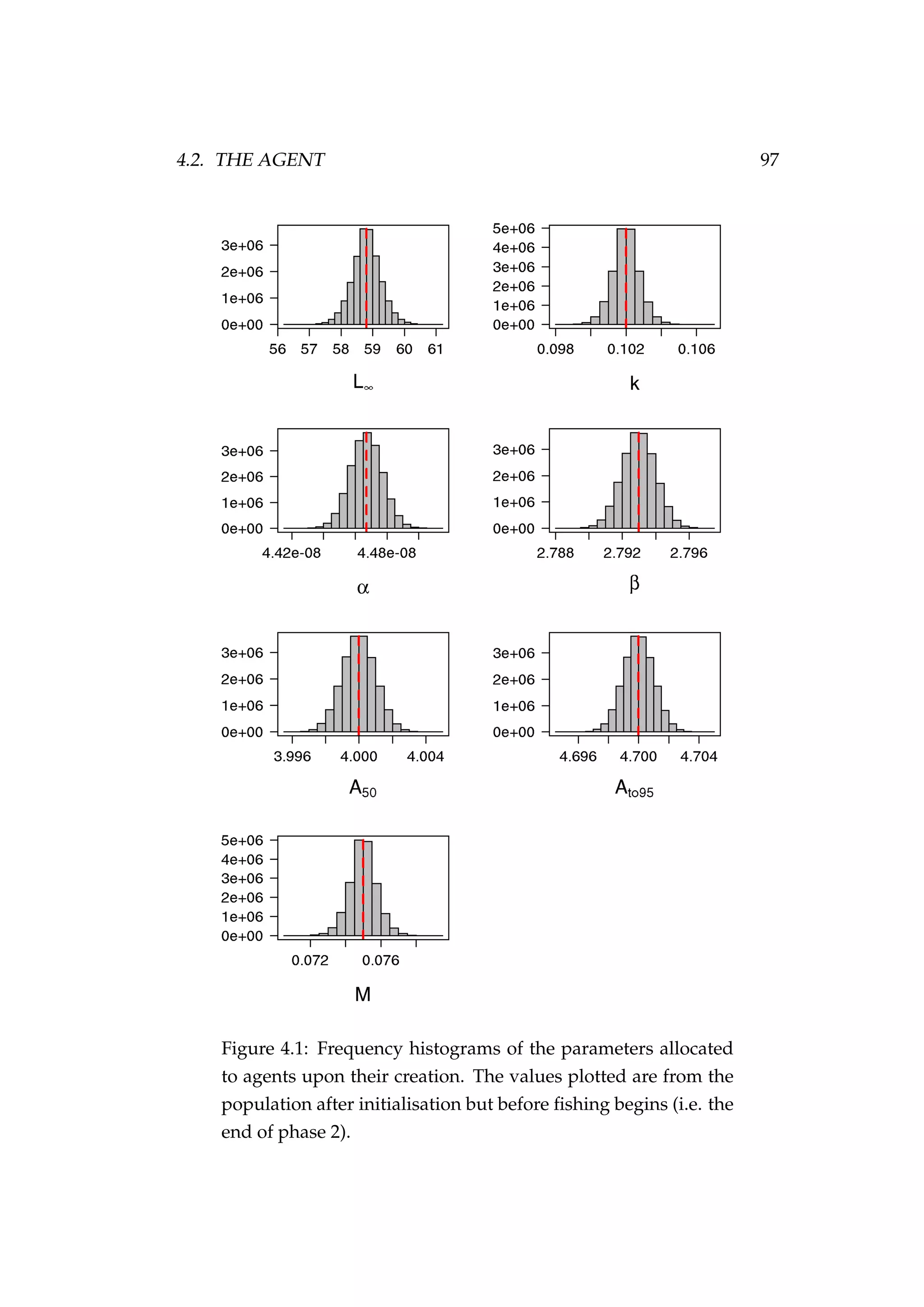
27. 1.2. NOTATION, TERMINOLOGY AND LAYOUT 15
• A new process model for modelling the dynamics of fish tagged us-
ing pop-up satellite archival tags coupled with a new observation
model for geolocating fish using depth/bathymetric data (Chapter 6)
• Bayesian emulators nested within a state-space framework (Chap-
ter 7)
• Further development of stochastic Bayesian emulators and a proof of
concept applied to a spatially explicit agent based model (Chapter 7).
1.2 Notation, terminology and layout
This section describes some of the mathematical terminology used
throughout this thesis.
Generally a bold capital symbol A refers to a matrix, a bold lowercase
symbol a to a vector and an unbolded italic symbol a to a scalar. {ai}n
i=1
is an ordered n-tuple. θ and θ are generally used to represent a parameter
or parameter vector, respectively. Data are usually denoted y. R is a real
number.
The expected value of a random variable a is E[a], while V[a] is the vari-
ance of a, and C[a] is the covariance of a. The terms π(·), p(·) or P(·) repre-
sent probability distributions. iid is short for independent and identically
distributed. a|b means event a conditional on event b having occurred. The
symbol ∀ means for all values, usually referring to all of the values within
an ordered tuple.
Throughout we use σ for standard deviation and σ2
for variance. A normal
distribution with mean µ and variance σ2
is written N(µ, σ2
). We use U to
represent a uniform distribution, IG inverse gamma, log N log-normal,
Bin binomial, and Ga gamma. Other distributions are defined as they are
used. The random variable ε is usually used to represent an error term.
It is common to see log-normal errors applied in fisheries science (typically
used for innovations). For example, if we have a random variable α that is
assumed to be log-normally distributed with standard deviation σ we can

28. 16 CHAPTER 1. INTRODUCTION
write
αt = αt−1eη
where η ∼ N −σ2
/2, σ2
,
or
αt = αt−1eε−σ2/2
where ε ∼ N 0, σ2
,
noticing the −σ2
/2 adjustment. In both cases log(αt) = log(αt−1) + η, but
E[αt|αt−1] = αt−1 only if η ∼ N(−σ2
/2, σ2
) (see Appendix A.2, page 323).
Without this adjustment the expected value of a random variable α will
tend to increase. However, if σ is small, say σ = 0.01, then the effect can be
negligible (i.e. e−0.012/2
= 0.99995) so sometimes the adjustment is omitted
in the literature.
Throughout this document we use boxes, like the one below, to develop
ideas alongside the text.
Boxes like this are used to illustrate ideas or concepts alongside the
text.
If you are viewing this document electronically as a pdf then it is useful
to know that all references to acronyms, appendices, chapters, cited liter-
ature, contents entries, equations, figures, pages, sections, and tables are
hyperlinked (i.e. clicking on the reference will take you to the relevant
part of this document). Any web-sites referred to in the text are also hy-
perlinked and clicking the link will open the web page in your default web
browser.
A glossary of acronyms, technical terms and commonly used fisheries pa-
rameters is also provided. The words contained in the glossary are also
hyperlinked throughout this document. If the reader is ever unsure of a
word then clicking the word will take the reader to the relevant glossary
entry (if that word is in the glossary, this can be checked by hovering a
mouse cursor over the word and if the cursor changes then that word is
in the glossary). The glossary lists hyperlinked page numbers to all of the
pages containing these words.
This thesis is fully version controlled on GitHub (https://github.
com/quantifish/PhD).

29. 1.3. COMPONENTS OF A FISHERIES MODEL 17
1.3 Components of a fisheries model
If Bt is the total biomass (e.g. tonnes) of a fish population at time t, Nt is
the total number of individuals within that population at time t, and wt is
the mean weight (tonnes) of a single fish at time t, then
Bt = Ntwt (t = 0, . . . , T).
A fisheries model provides a mathematical or statistical description of the
way Bt and Nt evolve over time, and specifically, how that population
responds to anthropogenic removals (exploitation)1
. Often these models
are tailored to suit both the population in question and the data that are
available. The components of these models, the way that these models can
be structured, and the types of data that are used to inform them follows.
Many of the equations in this section are drawn from Bull et al. (2012).
1.3.1 The partition
Often in models of a fish population we specify Na,t individuals of age a
in year t. We can in general represent counts of fish in any given year as a
matrix of numbers of fish where the columns are either age-classes (often
referred to as cohorts) or size-classes, and the rows are defined by some
categorisation, such as sex, maturity, area, stock, or tag year. We call this
matrix the “partition” (e.g. Table 1.1). In a model, the partition is updated
over time by applying suitable transformations. For example, to age the
fish after one year we simply move all of the fish in the partition one cell
to the right
Na,t = Na−1,t−1 (a = amin, . . . , A), (1.1)
and absorb all of the oldest fish into a single final age group A
NA,t = NA−1,t−1 + NA,t−1. (1.2)
This is how the numbers of fish in stock assessment models have been
viewed conceptually for some time, but R.I.C.C. Francis (NIWA) coined
1
Not all fisheries models express the abundance of fish in a population as a biomass;
some simply track the numbers of fish through time.

30. 18 CHAPTER 1. INTRODUCTION
Table 1.1: An example in which the partition (Na,m,s) is a ma-
trix filled with numbers of fish at age a, up to a maximum age
A, for different categories. Here the categories structure the
population by sex s (female, male) and maturity m (immature,
mature).
Age (a)
1 2 ... A − 1 A
Immature Female ...
Immature Male ...
Mature Female ...
Mature Male ...
the term partition to describe the population matrix. Consequently, the
use of the term is mainly limited to New Zealand literature.
The partition can be used in combination with other information to de-
rive properties of the population. For instance, the mean weight of each
individual in the partition at age a is wa, so by summing the product of
numbers-at-age and weight-at-age we can derive the total biomass of the
population
Bt =
a
Na,twa. (1.3)
Sex in the partition
Sex is included in the partition so that processes within the stock assess-
ment can be sex-specific. For instance, different growth models may be
applied to females and males, or the spawning stock biomass might be
calculated as the biomass of mature females only. If sex is not included
in the partition (i.e. we choose a single sex model) we are effectively as-
suming that the fish are reproducing asexually. This is often a reasonable
approximation to the truth, particularly if there is little difference between
the sexes in their sizes and spatial distribution.

31. 1.3. COMPONENTS OF A FISHERIES MODEL 19
1.3.2 Length and weight at age
Length and weight data from the commercial catch are perhaps the most
commonly available data in fisheries, because they are the cheapest and
easiest to collect. When analysed in conjunction with age data, one can
construct growth curves that inform us of the mean length or weight of
a fish at a given age. In many fish species, the age can be determined
by examining the otolith and counting the rings (much like the growth
rings of a tree). The ability to easily age a fish often determines whether
an age-structured or length-based model will be used (see Section 1.4,
page 34 for details on these different model structures). The relationship
between length or weight and age is often described deterministically us-
ing a growth model. The purpose of these growth models is to provide an
estimate of the expected length of a fish for a given age. Perhaps the most
commonly used growth model is that proposed by von Bertalanffy (1934)
La = L∞ 1 − e−k(a−t0)
, (1.4)
where La is the mean length (cm) of an individual in the population at
age a, L∞ is the asymptotic length or the mean length of very old organ-
isms (cm), k is the Brody growth coefficient (a curvature parameter that
describes how fast the organism approaches L∞ with units years−1
), and
t0 is the growth intercept (the hypothetical age at which the organism has
zero length with units years, e.g. Figure 1.1). The parameter t0 need not
be 0 since fish are only caught at ages > 0, and a good fit of this sim-
ple model may require t0 = 0 without ever predicting a fish of negative
length within a stock assessment model. These parameters are typically
expressed in centimetres (cm) and years, but may take other units. When
fitting this model, we estimate the parameters L∞, k and t0 given a sample
of fish of known age a and length La.
However, this growth function may not be the best curve to describe the
growth of a particular species. There are many other growth models that
may be more suitable (e.g. Richards 1959, Gompertz, logistic, exponential).
Moreover, such growth curves model the mean and variability of growth
in the population, but not the trajectories of individuals.

32. 20 CHAPTER 1. INTRODUCTION
Figure 1.1: Length-at-age example plot using the von Berta-
lanffy growth model (Equation 1.4). The parameter values for
this model are given in the bottom right of the figure.
In most stock assessment models it is necessary to determine the weight-
at-age of individuals in the population. We can do this using a power law
length-weight relationship
wa = αLβ
a. (1.5)
The exponent β is close to 3.0 for most species while the coefficient α varies
between species. If the exponent β is greater than three for a certain fish
species, that species tends to become relatively fatter or have more girth
as it grows longer. If the exponent β is less than three, the species tends
to be more streamlined. Alternatively, the length-weight relationship may
be combined with the von Bertalanffy relationship (Equation 1.4),
wa = w∞ 1 − e−k(a−t0) β
, (1.6)
where wa is the mean weight (tonnes) of a fish at age a, α and β are pa-
rameters of the length-weight relationship, w∞ is the asymptotic weight
(tonnes) of fish in the population which may be found using w∞ = αLβ
∞,
k is the Brody growth coefficient (years−1
), and t0 is the growth intercept
(years) (e.g. Figure 1.2).

33. 1.3. COMPONENTS OF A FISHERIES MODEL 21
Figure 1.2: Examples of the length-weight relationship (left,
Equation 1.5) and weight-at-age (right, Equation 1.6). The pa-
rameter values used are given in the bottom right of each fig-
ure.
1.3.3 Maturation
Maturation is the process in which immature fish become sexually mature
and therefore able to reproduce. This process can be modelled in one of
two ways in a stock assessment model, by including maturity in the parti-
tion, or not including maturity in the partition. If maturity is included in
the partition, then as fish become mature they can be moved accordingly
within the partition. One function that may be used to achieve this is the
logistic-producing ogive
ηa =



0 if a < L
λ(L) if a = L
(λ(a) − λ(a − 1))/(1 − λ(a − 1)) if L < a < H
1 if a ≥ H
, (1.7)
where
λ(a) = 1 1 + 19(A50−a)/Ato95
,

34. 22 CHAPTER 1. INTRODUCTION
where ηa represents the proportion of immature fish at age a maturing
each year (0 ≤ ηa ≤ 1) and not the proportion of fish mature in that year.
The logistic-producing ogive has the parameters L, H, A50 and Ato95. L
and H are used to define the age at which no fish are mature and the age
at which all fish are mature, respectively. A50 and Ato95 describe the age
at which 50% of individuals within the population are mature and the
difference in age at which 95% of individuals within the population are
mature, respectively.
When maturity is not explicitly included in the partition a parametric dis-
tribution can be used to describe the proportion of mature fish in each age-
or size-class at any given time. This approach assumes that the proportion
of mature fish remains constant over time. A logistic ogive is commonly
used to model maturity when maturity is not included in the partition
ma = 1 1 + 19(A50−a)/Ato95
(0 ≤ ma ≤ 1), (1.8)
where ma is the proportion of individuals at age a that are sexually ma-
ture, and A50 and Ato95 are parameters describing the age at which 50% of
individuals within the population are mature and the difference in age at
which 95% of individuals within the population are mature, respectively
(e.g. Figure 1.3).
Note that Equation 1.8 can be written
ma = 1 1 + exp −
a − A50
Ato95
log(19) ,
logit (ma) =
a − A50
Ato95
log(19),
where logit(p) ≡ log
p
1 − p
.
1.3.4 Natural mortality
Natural mortality is the death of fish due to causes not associated with
fishing (e.g. cannibalism, competition, disease, old age, predation). Nat-

35. 1.3. COMPONENTS OF A FISHERIES MODEL 23
Figure 1.3: Example of the logistic ogive used to model matu-
rity (Equation 1.8). The parameter values used are given in the
bottom right of the figure. The dashed lines represent the ages
at which 5%, 50% and 95% of the population are mature.
ural mortality is usually applied as an instantaneous rate and the propor-
tion surviving a time interval of τ years2
is e−τM
, where M is the natural
mortality rate3
. It is often assumed that M is independent of age and year
(an exception to this can be found in the New Zealand hoki stock assess-
ment where M is modelled as being age-dependent Ma, see Francis 2006).
Natural mortality is one of the most difficult parameters to estimate, par-
ticularly when we have only a short time series of observations, and is a
crucial element of a stock assessment (Hewitt et al. 2007). In New Zealand
M is usually fixed and assumed known within stock assessment models
(i.e. not estimated). However, in countries with much longer fishery time-
series (e.g. the US) M is sometimes estimated within stock assessment
models.
2
In most models we would specify 0 ≤ τ ≤ 1 because mortality is calculated from year
to year. However, we could potentially develop a model that tracks numbers in multiple
year time-steps.
3
It is also interesting to note that the mean age of fish in a model is 1
M .

36. 24 CHAPTER 1. INTRODUCTION
1.3.5 Fishing mortality
Fishing mortality is the removal of fish from a population due to fishing
activities using fishing gear (fishing activities could be commercial, recre-
ational, customary or illegal). The catch biomass (Ct) during year t is di-
rectly removed from the population in biomass dynamics models (see Sec-
tion 1.4.1, page 35) or used to derive an exploitation rate (Ut) or a fishing
mortality (Ft) in statistical catch at age models (see Section 1.4.2, page 37).
Age or length dependent selectivity functions can be used in these mod-
els to remove the relative proportion of these fish from the age or length
partitions in the model (see Section 1.3.9, page 27).
1.3.6 Spawning stock biomass (SSB)
The spawning stock biomass (SSBt) is the biomass (tonnes) of mature fish
within a fish stock at time t and can be determined by
SSBt =
a
Na,twamae−τM
, (1.9)
where Na,t is the number of fish of age a at time t, wa is the mean weight
(tonnes) of a fish at age a, ma is the proportion of fish mature at age a, M
is the natural mortality rate, and τ is used to set the time of year we wish
to calculate SSBt. By convention, the SSB is often assumed to be a mid-
season estimate, and hence we set τ = 0.5 on the assumption that natural
mortality occurs at a constant rate throughout the year. This would give us
the mid-year SSB by applying half of the natural mortality (e−0.5M
) before
calculating SSBt.
1.3.7 Recruitment
Recruitment is the addition of new individuals to the fished component
of a stock. Fish usually recruit to the fished (vulnerable) component of a
stock when they reach a size, or age, sufficient to be caught by the fishing
gear used. In an age-based model, all recruiting fish are of some speci-
fied minimum age (amin). This minimum age is usually the lower of some

37. 1.3. COMPONENTS OF A FISHERIES MODEL 25
approximate age corresponding to a minimum catchable size and the age
for which the analyst wishes to report results for (and is almost always
assumed to be age 1).
The number of fish that recruit to a stock at time t is usually assumed to
be dependent on some underlying average annual recruitment in the un-
fished population R0 (numbers of fish, see Section 1.3.8, page 27), the SSB
(biomass rather than numbers) of fish during time t − 1, and the strength
(a multiplier) of the year class (cohort) during time t. The recruitment Rt
(number of fish) at time t can be written
Rt = R0 × SR(SSBt−te ) × YCSt, (1.10)
where te is the number of time-steps after spawning that a year class (co-
hort) enters the fished component of a stock and can incorporate egg de-
velopment time as well as the time taken for the fish to reach recruitment
age amin (usually te = 1), SR(·) is a function of the SSB, and is a measure
of the productivity of a spawning biomass of the stock, SR(SSBt−te ) is the
stock recruitment value at time t − te, and YCSt is the relative year class
strength (YCS) at time t. This allows environmental/ecological variations
to lead to higher or lower numbers of recruits in a given year.
The stock recruitment function SR(·) is used to model the relationship be-
tween SSB and the number of recruits (Rt) entering the fishery each year.
The stock recruitment function scales R0, the stock’s expected average re-
cruitment if there had been no anthropogenic mortality. The two most
commonly used stock recruitment functions are those developed by Bev-
erton & Holt (1957) and Ricker (1954). The Beverton-Holt function is
SR(SSBt) =
SSBt
B0
1 −
5h − 1
4h
1 −
SSBt
B0
, (1.11)
and the Ricker function is
SR(SSBt) =
SSBt
B0

 1
5h
5
4
SSBt
B0
−1

 , (1.12)
where SR(SSBt) is the stock recruitment value at time t (0 ≤ SR(SSBt)),
SSBt is the SSB (tonnes) at time t, B0 is the initial biomass (tonnes), and h is

38. 26 CHAPTER 1. INTRODUCTION
Figure 1.4: Examples of Beverton-Holt (left, Equation 1.11) and
Ricker (right, Equation 1.12) recruitment. The parameters used
are given in the bottom right of each figure.
the steepness parameter defined as h = SR(0.2B0) (e.g. Figure 1.4, Mangel
et al. 2010).
Although recruitment could be defined using just R0 and the stock recruit-
ment relationship SR(SSBt) (i.e. Rt = R0 × SR(SSBt−te )), we know that
the true numbers of fish recruiting to a stock each year in the absence of
fishing would vary about R0 (e.g. see Section 1.3.8 below). To account for
this we use YCS multipliers (also known as recruitment multipliers). The
YCS multipliers allow the recruitment to vary between year’s within the
model while maintaining the definition of R0 (i.e. the number of recruits
that would be observed, on average, in the absence of fishing, e.g. see
Figure 1.5). The year class (cohort) strengths can be defined as
YCSt = eεR
t −σ2
R/2
where εR
t ∼ N 0, σ2
R , (1.13)
and σ2
R is the recruitment variance.

39. 1.3. COMPONENTS OF A FISHERIES MODEL 27
Figure 1.5: Example of year class strength multipliers YCSt
(left, Equation 1.13) and recruitment Rt (right, Equation 1.10).
The parameters used are given in the top left of each figure. In
the recruitment plot (right) the YCSt from the left plot is used
and SR(SSBt) = 1 ∀t.
1.3.8 R0 and B0
The stock’s average unfished recruitment R0 (numbers) and average
biomass B0 (tonnes) are perhaps the two most important parameters in
stock assessment models. R0 is the underlying parameter that determines
how large a stock would be, on average, if there had been no fishing. From
R0 one can calculate B0, which is defined as the SSB that would exist if
recruitment were equal to R0 every year and there was no fishing (see
Equation 1.20). It is often assumed (e.g. for the purposes of initialising
simulations) that B0 = SSBt=1. Figure 1.6 illustrates the definition of B0.
1.3.9 Selectivity
Selectivity refers to the relative vulnerability of fish of different ages or
sizes to the fishing gear used. Although we often assume that selectivity
is independent of time, this is likely to be an unrealistic assumption as

40. 28 CHAPTER 1. INTRODUCTION
Figure 1.6: The definition of B0. The solid line represents the
actual biomass of a fish population that would occur in the ab-
sence of fishing. This example illustrates a population with a
cyclic biomass, however the biomass of a real population may
take any form. The horizontal dashed line represents B0 or the
mean biomass that would exist in the absence of fishing. The
two vertical dotted lines represent the time period of fishing or
the set of years S for which we wish to define R0.

41. 1.3. COMPONENTS OF A FISHERIES MODEL 29
fishing gear can improve over time or the fleet can fish in different areas
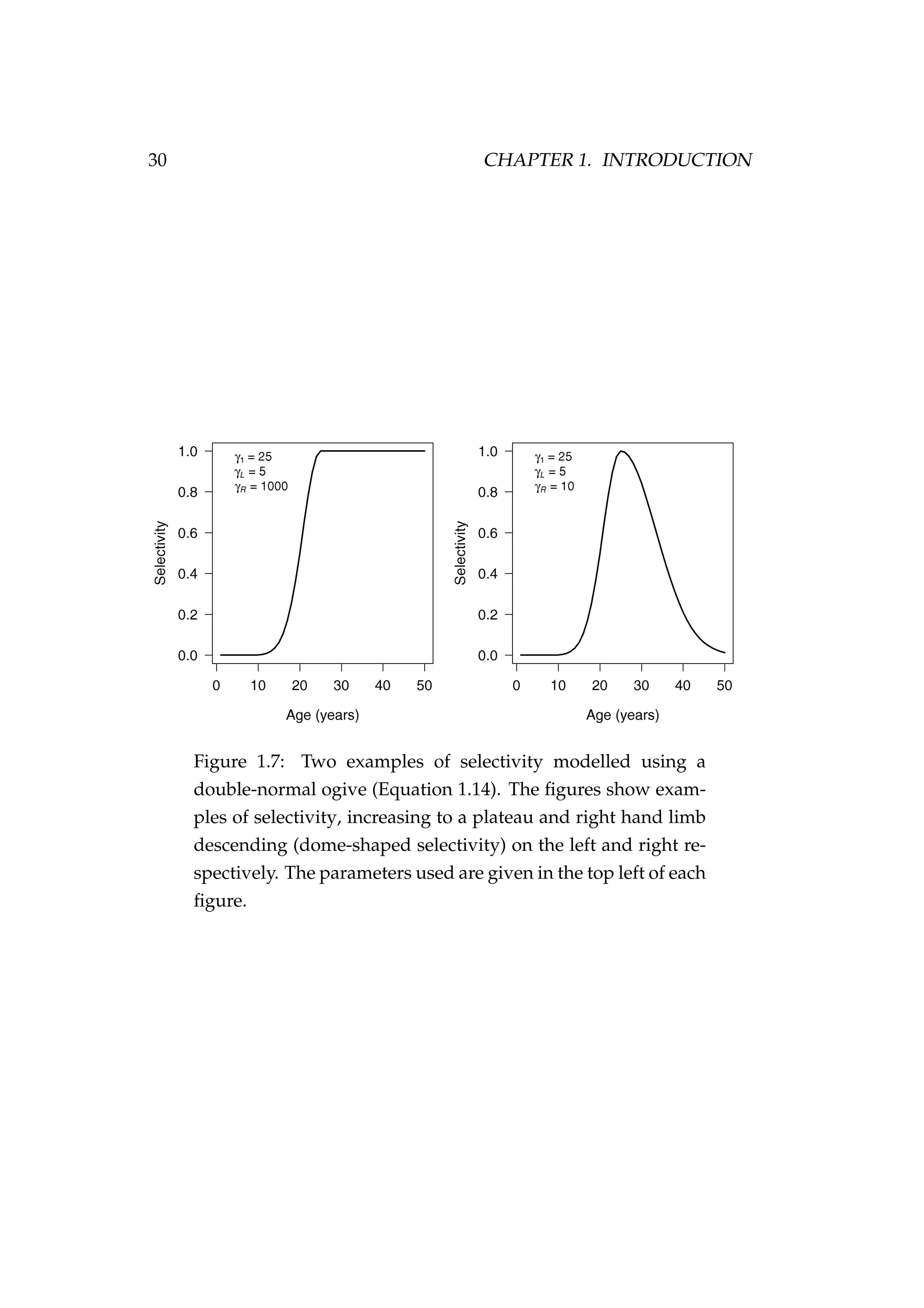
and have differing degrees of success. Below is an example of selectivity
parameterised using a double-normal ogive
Sa =



2−[(a−γ1)/γL]2
if a ≤ γ1
2−[(a−γ1)/γR]2
if a > γ1
, (1.14)
where Sa is the selectivity (proportion of fish vulnerable) of fish in the
population at age a, γ1 is the mode, γL describes the shape of the left hand
limb, and γR describes the shape of the right hand limb (e.g. Figure 1.7).
The scale of selectivity is arbitrary and Sa is scaled to have a maximum
value of 1.
Note that Equation 1.14 can be written
Sa =



e
−
a−γ1
γL
2
log(2)
if a ≤ γ1
e
−
a−γ1
γR
2
log(2)
if a > γ1
.
The double-normal ogive is useful as it allows the model to specify the
parameters γ1, γL, and γR, in such a way that selectivity can approximate
a logistic curve or have a declining right hand limb (dome-shaped). “Lo-
gistic” type selectivities suggests that younger/smaller fish are less vul-
nerable to the fishing gear used in the fishery than the older/larger fish.
This could be because the younger fish are small enough to fit through the
mesh in a trawl net and escape, too small to take the bait on a longline,
or may live elsewhere. A dome-shaped selectivity suggests that younger
fish are less vulnerable than middle aged fish, and that the vulnerability of
fish decreases again as they grow older. This may occur if the oldest fish
in the population are alive, but are not vulnerable to the fishery for some
reason (e.g. they live somewhere else, they are large enough to outrun a
trawl net, or are big enough to simply pull the hook off a longline).
Selectivity may also be parameterised in a way that allows it to vary over
time (e.g. Butterworth et al. 2003, Ianelli et al. 2013, Nielsen & Berg 2014).
However, estimating the selectivity of each age group every year as indi-
vidual parameters could potentially result in hundreds of selectivity pa-

42. 30 CHAPTER 1. INTRODUCTION
Figure 1.7: Two examples of selectivity modelled using a
double-normal ogive (Equation 1.14). The figures show exam-
ples of selectivity, increasing to a plateau and right hand limb
descending (dome-shaped selectivity) on the left and right re-
spectively. The parameters used are given in the top left of each
figure.

43. 1.3. COMPONENTS OF A FISHERIES MODEL 31
rameters. Ianelli et al. (2013) estimated selectivity in this way for the East-
ern Bering Sea walleye pollock stock assessment but restricted the amount
of change from year to year (in each age) by treating the selectivity in each
age group as a random walk4
Sa,t = Sa,t−1eγt−σ2/2
where γt ∼ N(0, σ2
S). (1.15)
Treating the temporal component of selectivity as a random walk in this
way could allow selectivity to “creep” or change in some structured way
over time. However, the values allowed for the variance hyperparame-
ter σ2
S would need to be considered carefully to avoid overfitting of the
model. Alternatively, the random-walk or random-effect concept could be
imposed on the parameters of a selectivity ogive. For example, Ianelli et al.
(2013) implemented the logistic ogive as a random walk using
Sa,t = 1 + e−aαt−βt
−1
,
αt = ¯αeδα
t where δα
t − δα
t−1 ∼ N(0, σ2
δα ),
βt = ¯βeδβ
t where δβ
t − δβ
t−1 ∼ N(0, σ2
δβ ).
In any case, care should be taken if implementing time-varying selectivity
and selectivity models should be evaluated carefully (Maunder & Harley
2011, Punt et al. 2014).
1.3.10 Areas, stocks and fisheries
Several terms are used in fisheries science that can be confusing, especially
the terms “area”, “stock”, and “fishery”. So far only single-area, single-
stock models have been discussed. However, there are many other ways to
structure a stock assessment model. For example, we can have single-area
single-stock multi-fishery models (e.g. Antarctic toothfish, Mormede &
Dunn 2014), or multi-area multi-stock multi-fishery models (e.g. snapper
in SNA 1, see Francis & McKenzie 2013). Here we introduce the concepts
of areas, stocks and fisheries.
4
Actually, the equation presented in Ianelli et al. (2013) was Sa,t = Sa,t−1eγt
but we
have added in the −σ2
/2 for consistency.

44. 32 CHAPTER 1. INTRODUCTION
Areas
Areas z ∈ Z define non overlapping geographic regions of a popula-
tion. When multiple areas are defined within a model then the location
or movement of fish between areas must be specified. Location is usually
used for sessile organisms (i.e. animals that don’t move like paua), but do
recruit to different areas within the model. Movement is typically mod-
elled as a migration, usually using a z × z matrix for each partition that
specifies the proportion of the numbers of fish within each area Na,z that
move in a given time step. The migration matrix will often differ between
ages and sex (i.e. a z × z matrix for each age or sex).
Stocks
A stock is a biological production unit in which the effects of emigration
and immigration can be considered negligible. However, in fisheries mod-
els, this definition is often blurred. Stocks j ∈ J define the different spawn-
ing sub-populations within a fishery. In a multi-area, single-stock model
the spawning stock biomass of the stock is simply determined by sum-
ming the biomass of all mature fish in all areas
SSBt =
a,z
Na,t,zwama (1.16)
where Na,t,z is the number of fish of age a at time t in area z. In a multi-
area, multi-stock model there are a number of ways that the spawning
stock biomass could be derived. The first way is to sum the biomass of
mature fish in each area to obtain a spawning stock biomass for each of
these areas
SSBt,z =
a
Na,t,zwama. (1.17)
Alternatively, fish from different stocks may contribute towards reproduc-
tion only if they are present in their stock area at the time of spawning. In
this case it is necessary to introduce the subscript j to indicate which stock
the fish came from
SSBt,j =
a
Na,j,t,zwama. (1.18)

45. 1.3. COMPONENTS OF A FISHERIES MODEL 33
Fisheries
A fishery f ∈ F is an action applied to a fish stock or area. The fishery
removes biomass from the stock as catch. We may have multiple fisheries
in a single area, each fishery having a distinct selectivity and operating
on a particular set of fish species. Stock assessments often represent spa-
tial structure through a “fisheries-as-areas” approach whereby multiple
fisheries, each with different selectivity patterns, are used as a proxy for
spatial availability.
1.3.11 Simulation
To run a statistical catch-at-age model (see Section 1.4.2, page 37), we spec-
ify the minimum age (amin) of the fish to be modelled, the final age (A) if
a plus group is to be used, the average unfished recruitment in numbers
of fish (R0) and the natural mortality rate (M). In the absence of fishing
we assume that there is some (equilibrium) carrying capacity (B0). We
evaluate B0 numerically by running a simulation of the model over a long
period until it reaches equilibrium. This allows us to determine the initial
age structure (N0
a ) of the population before fishing. We call this initial age
structure the initial state and the process of solving for the initial state is
called initialisation. The initial state can be found by solving for N0
a
N0
a =



R0e−(a−1)M
if a = amin, . . . , A
∞
a=A R0e−(a−1)M
if a = A
.
This equation actually has an analytic form that is found using geometric
series
N0
a =



R0e−(a−1)M
if a = amin, . . . , A
R0
eM−AM
1−e−M if a = A
, (1.19)
see Appendix B.1 (page 327) for the proof. From this B0 is calculated mid-
year as
B0 =
a
N0
a wamae−0.5M
. (1.20)

46. 34 CHAPTER 1. INTRODUCTION
where wa is the mean weight at age and ma is the maturity at age. Fig-
ure 1.8 shows an initial age structure, with a plus group at 50 years of age.
Figure 1.8: Example of the initial state or initial age structure
of a population (Equation 1.19). The 50+ refers to the use of a
plus group (i.e. the sum of fish aged 50 and above) and is the
reason why more fish are found in this age group than some of
the earlier age groups. The parameters used are given in the
top right of the figure.
1.4 Types of model
Two modelling structures are commonly employed for assessing the dy-
namic response of fish populations to exploitation; biomass dynamic mod-
els, and age- or length-structured models. However, in the last few years
individual-based models have increased in popularity. Biomass dynamics
models, age- or length-structured models, and individual-based models
represent a spectrum of how we group or bin fish in our models. These
models range from lumping the total biomass of fish within a given year
together in biomass dynamic models, to modelling the age structure of co-

47. 1.4. TYPES OF MODEL 35
horts in age-structured models or groups of fish of similar length in length-
structured models, to accounting for each individual fish within a popu-
lation in individual-based models. However, it is entirely possible for the
modeller to bin fish together anywhere along this spectrum, for example,
age-structured models are somewhere between biomass dynamics models
and individual-based models because they bin fish together according to
their age.
1.4.1 Biomass dynamics models
Biomass dynamic models, also known as production models or surplus
production models, are the simplest stock assessment models that are
commonly used. These models consider the net effects of recruitment,
growth, and mortality on the entire population each year. The Schaefer
surplus production model (Schaefer 1954) is perhaps the most widely used
biomass production model and can be written
Bt = Bt−1 + g (Bt−1) − Ct−1, (1.21)
g (Bt) = rBt 1 −
Bt
K
,
where Bt is the biomass of the stock (tonnes) at time t, g(Bt) is a function of
biomass known as the surplus production (tonnes) at time t, Ct is the catch
(tonnes) at time t, r is an intrinsic rate of population growth (unitless), and
K is the carrying capacity (tonnes), a parameter which corresponds to the
unfished equilibrium stock biomass.
In biomass dynamics models (and age-structured models) it is usually as-
sumed that the catch (Ct) is proportional to the stock biomass (Bt) and
fishing effort (Et)5
Ct = qEtBt, (1.22)
5
In biomass dynamics and age-structured models the catch (Ct) is usually treated as
a covariate (i.e. known without error) and the catch per unit effort (It) is usually treated
as data (i.e. an outcome variable). This suggests that we determine the catch (Ct) in
advance, and then discover how much effort (Et) is required to observe this catch, and
hence observe It = Ct
Et
.

48. 36 CHAPTER 1. INTRODUCTION
where Et is the fishing effort (year−1
), and q is a dimensionless parameter,
known as the catchability coefficient, that describes the effectiveness of
each unit of fishing effort (see Equation 1.41). Equation 1.22 implies that
the catch per unit of fishing effort (It) is an index proportional to stock
abundance (Bt, see Equation 1.42)
It =
Ct
Et
= qBt, (1.23)
or
It = q
1
2
(Bt + Bt+1) .
There are many other forms of biomass dynamics models including:
the Pella & Tomlinson (1969) model where
g (Bt) =
r
z
Bt 1 −
Bt
K
z
,
which includes the additional shape parameter z; the form suggested
by Fox (1970)
g (Bt) = rBt 1 −
log (Bt)
log (K)
;
difference models (Walters & Hilborn 1976); and regression methods. All
of these models pool aspects of production (i.e. recruitment, growth and
natural mortality) into the single production function g (Bt). Biomass dy-
namics models might be considered a crude over-simplification of a pop-
ulation because they may ignore too many details to produce reliable es-
timates of the population biomass. In fisheries without age data, or eas-
ily distinguished cohorts, they may nevertheless be useful for estimating
population trends. We use a biomass dynamics model later in Chapter 5
(page 137).
1.4.2 Age- and length-structured models
A significant improvement over biomass dynamics models are models
that incorporate age- or length-structured data. Current fisheries stock
assessments are mainly based on two approaches, both relying on catch-
at-age or catch-at-length data: statistical catch-at-age or -length models
(SCA or SCL) and virtual population analysis (VPA).

49. 1.4. TYPES OF MODEL 37
Virtual population analysis (VPA), also known as cohort analysis, uses
recursive algorithms to calculate past stock abundances based on past
catches with no underlying statistical assumptions. VPA can give unre-
liable estimates for cohorts that have not completely disappeared from
the fishery, and it requires an assumption about the natural mortality
rate (Hilborn & Kennedy 1992). We do not discuss VPA further.
Statistical catch-at-age models (SCA)
Statistical catch-at-age (SCA) models provide more formal methods for es-
timating the current abundance of cohorts still being fished and synthesise
many aspects of fisheries theory. SCA models commonly estimate a sepa-
rate recruitment for every year and every initial age class, and two to four
selectivity parameters for every fishing fleet, depending on available data.
Furthermore, these models can easily be extended to include spatial or
economic components when additional complexity is required. Bayesian
methods are often used in SCA models to describe uncertainty, and in-
clude prior distributions for parameters derived from meta-analysis. A
major impetus for using SCA models is their ability to integrate almost
any form of data.
Here we present an example of a general SCA model using the exploitation
rate formulation (but see page 44 for an alternative catch equation). We
present this model for a single time-step t (normally this would be a single
year). If Na,t is the number of fish of age a at time t then the fish can be
aged at the beginning of the year using
Na,t = Na−1,t−1,
where Na,t is the numbers at age after ageing (Equations 1.1 and 1.2).
Next, fish recruit to the population using the recruitment function (Equa-
tion 1.10). Given R0, last years spawning stock biomass SSBt−1, and the
stock recruitment function SR(·), the number at age after recruitment is
Na=1,t = Rt = R0 × SR(SSBt−1) × eεR
t −σ2
R/2
where εR
t ∼ N 0, σ2
R .
Now we apply half of the natural mortality Ma,t to the population
Na,t = Na,te−0.5Ma,t
,

50. 38 CHAPTER 1. INTRODUCTION
where Na,t is the mid-year numbers at age. We can now calculate a series
of mid-year biomasses (all with units tonnes). If wa,t is the mean weight
(tonnes) of a fish of age a at time t (during the middle of the year), then the
total mid-year biomass at age Ba,t and the total mid-year biomass Bt is
Ba,t = Na,twa,t or Bt =
a
Na,twa,t.
If Sa,t is the selectivity of fish of age a at time t then the mid-year vulnerable
biomass at age Va,t and the total mid-year biomass that is vulnerable to the
gear used by the fishery Vt is
Va,t = Na,twa,tSa,t or Vt =
a
Na,twa,tSa,t.
The vulnerable biomass is the portion of a stock’s biomass that is available
to the fishery. If ma,t is the proportion of fish of age a at time t that mature,
then the mid-year spawning stock biomass at age SSBa,t and the total mid-
year spawning stock biomass SSBt is
SSBa,t = Na,twa,tma,t or SSBt =
a
Na,twa,tma,t.
Now this years exploitation rate at age Ua,t (actually the proportion of vul-
nerable biomass by number caught per annum, rather than by biomass) is
applied to the fishery, generating this years catch at age Ca,t as a biomass
(tonnes).
Ca,t = Ua,tVa,t,
or
Ua,t =
Ca,t
Va,t
=
Ca,t
Na,twa,tSa,t
.

51. 1.4. TYPES OF MODEL 39
This catch is removed from the population using
Na,t = Na,t (1 − Ua,tSa,t)
= Na,t 1 −
Ca,t
Va,t
Sa,t
= Na,t 1 −
Ca,t&
&Sa,t
Na,twa,t&
&Sa,t
= Na,t 1 −
Ca,t
Na,twa,t
= Na,t − &
&&Na,t Ca,t
&
&&Na,t wa,t
= Na,t −
Ca,t
wa,t
,
Finally, the remaining half of the natural mortality is removed
Na,t = Na,te−0.5Ma,t
,
before progressing to the next time-step t.
However, this general form is far from practical and several assumptions
need to be made before these models are useful. To identify these assump-
tions, we start again. As before, Na,t is the number of fish of age a at time
t. The fish are aged and new recruits are added to the population using
the recruitment function (Equation 1.10)
Na,t = Na−1,t−1,
Na=1,t = Rt.
Next, half of the natural mortality M is applied, but the assumption that
M does not change with age or time (Ma,t = M) is made
Na,t = Na−1,t−1e−0.5M
,
where Na,t is the mid-year numbers at age. Assuming that the weight
at age of fish does not change with time (wa,t = wa), the total mid-year
biomass Bt is
Bt =
a
Na,twa.

52. 40 CHAPTER 1. INTRODUCTION
Assuming that selectivity does not change with time (Sa,t = Sa), the mid-
year vulnerable biomass at age Va,t and the total mid-year vulnerable
biomass Vt is
Va,t = Na,twaSa,
Vt =
a
Na,twaSa.
Assuming that maturity does not change with time (ma,t = ma), the mid-
year spawning stock biomass SSBt is
SSBt =
a
Na,twama.
Finally, assuming that the exploitation rate is independent of age (Ua,t =
Ut), the catch at time t is
Ct =
a
Ca,t
=
a
UtVa,t
= UtVt, (1.24)
or
Ut =
Ct
Vt
The catch is removed from the population using
Na,t = Na,t (1 − UtSa)
= Na,t 1 −
Ct
Vt
Sa
= Na,t 1 −
CtSa
a Na,twaSa
.
Finally the remaining half of the natural mortality is removed
Na,t = Na,te−0.5M
.

53. 1.4. TYPES OF MODEL 41
In practice we never have very reliable estimates of Ca,t. We do know
Ct though, so we can state
Ca,t = Ctfa,t,
fa,t =
Ba,tSa
a Ba,tSa
=
Na,twaSa
a Na,twaSa
,
Na,t = Na,t 1 −
Ca,t
Na,twa
= Na,t 1 −
Ctfa,t
Na,twa
= Na,t 1 −
CtSaNa,twa
Na,twa a Na,twaSa
= Na,t 1 −
CtSa
a Na,twaSa
. (1.25)
Or, we can allow selectivity to be time-varying
Na,t = Na,t 1 −
CtSa,t
a Na,twaSa,t
.
Also, note if Ca,t = UtVa,t then we can also define the catch in numbers
(rather than tonnes) as
ˇCa,t =
Ca,t
wa
and
ˇVa,t =
Va,t
wa
= Na,tSa
therefore
ˇCa,t = Ut
ˇVa,t,
ˇCt = Ut
ˇVt = UtNa,tSa,
Na,t = Na,t − ˇCa,t = Na,t − Ut
ˇVa,t = Na,t − UtNa,tSa = Na,t(1 − UtSa).

54. 42 CHAPTER 1. INTRODUCTION
In summary, SCA models are implemented as
Na,t = Na−1,t−1 age the fish (Equations 1.1 and 1.2)
Nt=1,t = Rt recruitment (Equation 1.10)
Na,t = Na,te−0.5M
apply half of the natural mortality
Bt =
a
Na,twa total biomass
Vt =
a
Na,twaSa biomass vulnerable to fishing
SSBt =
a
Na,twama spawning stock biomass (Equation 1.9)
Ct = UtVt calculate the catch
Na,t = Na,t (1 − UtSa) remove the catch
Na,t = Na,te−0.5M
apply remaining half of the natural mortality
(1.26)
where Na,t represents the numbers at age a and time t after aging, Na,t after
recruitment, Na,t after half of the natural mortality, Na,t after fishing mor-
tality and Na,t at the end of the year after the remaining half of the natural
mortality. The total biomass, vulnerable biomass and exploitation rate are
calculated after aging, recruitment and half of the natural mortality. The
order in which ageing, recruitment, mortality and spawning are applied
in Equation 1.26 is simply an example and the order in which these pro-
cesses are applied in practice may differ depending on what species/stock
is being modelled.
Statistical catch-at-length models (SCL)
Statistical catch-at-length (SCL) models provide more formal methods for
estimating the current abundance of length-classes being fished. SCL
models are applicable when the animals cannot be aged or the growth
curve is indeterminate (i.e. t0, see Equation 1.4, cannot be estimated), or if
the primary source of data is length-composition observations. SCL mod-
els are much less common than SCA models.
The structure of SCL models is very similar to that of SCA models, except

55. 1.4. TYPES OF MODEL 43
that the basic dynamics are size- rather than age-structured and recruit-
ment is spread over several length-classes rather than just the minimum
age amin. The numbers of fish in size-class at time t in a SCL model is
N ,t where = 1, . . . , n and n is the number of size-classes. Alternatively
the vector Nt could be used. To move fish between length-classes due to
growth requires an n × n growth matrix X
X = X , =






X1,1 X1,2 . . . X1,n
X2,1 X2,2 . . . X2,n
...
...
...
...
Xn,1 Xn,2 . . . Xn,n






where X , = 1 ∀ , (1.27)
where X , represents the proportion of fish growing from the length-class
to length-class and has the property X , ≥ 0. The matrix X is often
constrained to prevent “negative growth” (i.e. fish that shrink, X , = 0 if
> )
X = X , =






X1,1 X1,2 . . . X1,n
0 X2,2 . . . X2,n
...
...
...
...
0 0 . . . Xn,n






where X , = 1 ∀ .
This implies that Xn,n = 1. A SCL model also requires specification of
the natural mortality and fishing mortality. The natural mortality may be
applied using an n × n diagonal survival matrix S
S = S , =







e−M
0 . . . 0
0
... . . . 0
...
...
...
...
0 0 . . . e−M







, (1.28)
and the fishing mortality an n × n diagonal matrix
Ht = H , ,t =







1 − S1Ft 0 . . . 0
0
... . . . 0
...
...
...
...
0 0 . . . 1 − SnFt







. (1.29)

56. 44 CHAPTER 1. INTRODUCTION
where S is the selectivity on size-class and Ft is the fishing mortality
during time t. Now we can write the numbers of fish in each length-class
the following year N ,t+1 as
N ,t+1 = R ,t + XT
, S , H , ,tN ,t
= R ,t + (XT
SHtNt) or
Nt+1 = Rt + XT
SHtNt, (1.30)
where Rt is a vector of the number of recruits (to each size-class) at the
start of year t.
Catch equations
The catch equation in SCA (and SCL) models can be formulated in two
different ways (Bull et al. 2012). The first option, instantaneous mortality,
applies half of the annual natural mortality, then applies the mortalities
from all fisheries instantaneously, then applies the remaining half of the
natural mortality. The second option is to use the Baranov catch equation,
in which natural and fishing mortality occur simultaneously. In both cases,
we often assume that Ma,t = M.
When using instantaneous mortality the fishery removals are applied us-
ing an exploitation rate Ut each year t. Thus Na,t, the number of fish of age
a in year t is
Na,t = Na−1,t−1e−0.5M
(1 − Ut−1Sa)e−0.5M
, (1.31)
where M is the natural mortality rate and Sa is the selectivity of the fishing
gear used for fish of age a. This model ages all of the fish in the partition
by one year (Na−1,t−1 ← Na,t reduced by all mortality) and updates the
year. This equation assumes that all fishing takes place instantaneously
during the middle of the year because Vt is calculated during the middle
of the year (i.e. after removing half of the natural mortality using e−0.5M
),
and that Ut is independent of age. Work by Mertz & Myers (1996) suggests
that age-structured models are largely insensitive to this assumption.
When using Baranov mortality the fishery removals are applied each year
t using the fishing mortality rate Ft (again independent of age). Thus Na,t,

57. 1.4. TYPES OF MODEL 45
the number of fish of age a in year t is
Na,t = Na−1,t−1e−Za−1,t−1
, (1.32)
and Ft can be found by solving the Baranov catch equation
Ct =
a
FtSa
Za,t
waNa,t 1 − e−Za,t
, (1.33)
where Za,t is the total annual mortality and is defined as Za,t = M + FtSa.
There is no closed form equation for Ft given the other parameters, so
this equation must either be solved numerically (e.g. using the Newton-
Raphson method, Press et al. 1986), approximated (e.g. Popes approxi-
mation, Pope 1972), or by treating the catches as observations with small
coefficients of variation, so that the Ft’s are estimated as parameters (speci-
fying small coefficients of variation forces the estimated catches to be close
to the observed catches).
There has been some debate in the literature over the use of instanta-
neous mortality and Baranov mortality equations (Branch 2009b, Branch
2009a, Francis 2010, Branch 2010). Put simply, both methods are wrong.
Instantaneous mortality models assume that all fishing occurs instanta-
neously at some time in the model, and it is obvious that this would never
be the case in reality. However, Baranov mortality models assume that
fishing occurs constantly throughout the year, which is also unrealistic as
fishing activity is never constant but instead fluctuates according to the
weather, price and availability of fish, and many other factors. Further-
more, due to the need for numerical methods, Baranov mortality equa-
tions result in more computationally expensive models.
1.4.3 Individual-based models
Individual-based models (IBMs) represent populations in which individ-
uals differ in their maturation, migration, growth, and mortality and fol-
low these individuals, or small groups of individuals (super-individuals
or agents, e.g. Scheffer et al. 1995), through their life history. Although

58. 46 CHAPTER 1. INTRODUCTION
it is a very flexible modelling approach, the computational overheads in-
volved in an individual-based model can overwhelm even the most pow-
erful computers. This can make some models infeasible particularly if
trying to estimate parameter values. However, new hybrid methods that
combine classical models with individual-based aspects may be the key to
solving such dilemmas (e.g. Gray et al. 2006).
The diversity of methods/equations that may be used in IBMs is enor-
mous so only a couple of examples will be given here (for further exam-
ples see Grimm & Railsback 2005, Kim et al. 2002 or Gray et al. 2006). In an
agent-based model we have fp
k,t individuals in agent k at time t. k could
refer to an individual, a group of individuals (super-individual), an age
group a, or a size-class . To determine the total number of individuals Nt
in an agent-based model in any given year we would use
Nt =
k
fp
k,t. (1.34)
There are several ways to apply processes (e.g. natural mortality) to indi-
viduals (or bins of individuals) within an IBM. Taking natural mortality
M as an example, for each year in the life of individual (or agent) k the
Bernoulli distribution can be used to determine if the individual survives.
The individual is alive if Yk,t is one or is dead if Yk,t is zero where Yk,t is
given by
Yk,t|Yk,t−1 = 1 ∼ Bern(1 − e−M
), (1.35)
conditional on Yk,t−1 = 1 (i.e the fish had to be alive in the first place).
While modelling populations as individuals or small groups of individ-
uals may come at a computational cost, the benefits may make it worth-
while. In species or populations with small numbers of individuals such
as dolphins or whales, such models make sense if the data is available as
the computational overheads will be reasonably low and complex behav-
ioral attributes can be built in. However, if modelling populations with
large numbers of individuals (e.g. fish) then there must be a good reason
to do so using IBM’s. Chapter 4 (page 89) of this this thesis presents an
agent-based model in some detail.

59. 1.5. DATA 47
1.5 Data
We commonly find two time series of observations in stock assessment.
The first is a history of catches removed from the stock. The second is
an index of abundance: some measure that indicates the size of the stock.
Other information such as knowledge of the age structure of the popu-
lation, individual growth rates, fecundity at different ages, breeding sea-
sons, or other basic biology is usually available and may be useful.
The purpose of observations in stock assessment is to inform the parame-
ters of the model. The values for some parameters within stock assess-
ment models usually cannot be determined from auxiliary information
(e.g. data that is not included in the stock assessment model), nor esti-
mated reliably by fitting a model to data and must, therefore, be prespeci-
fied (Magnusson & Hilborn 2007). Examples of these parameters include
natural mortality (M), the steepness of the stock-recruitment relationship
(h, Equation 1.11 or 1.12), and the variation in recruitment (σ2
R, Equa-
tion 1.13). These parameters are typically set using estimates from similar
species, other stocks of the same species, meta-analysis, expert opinion, or
some other method (e.g. see Figure 1.9).
The most common observations used to inform stock assessment models
are proportions in the commercial catch-at-age data and an abundance in-
dex (usually catch per unit effort or a trawl survey). Proportions in the
catch-at-age data inform the selectivity and age structure in stock assess-
ment models. The abundance index informs the stock biomass. Each of
these data types will be discussed below. Tag-recapture data is also briefly
described below as an alternative to abundance indices.

60. 48 CHAPTER 1. INTRODUCTION
Figure 1.9: The derivation of natural mortality (M) by J.G.
Pope. This illustrates the fact that 0.2 is a common, but some-
times unjustified, value for M.

61. 1.5. DATA 49
1.5.1 Proportions in the catch-at-age
The proportions at age in the catch ((Pa)t) can be derived from the popu-
lation as
λa,t = Na,tUtSae−0.5M
,
(Pa)t =
λa,t
a λa,t
where
a
(Pa)t = 1 ∀t, (1.36)
where λa,t is the vulnerable numbers (not biomass) at age a that are caught
at time t. The proportions at age in the catch ((Pa)t) for a single year t is
often referred to as an age-frequency. Observations of the proportions at
age may be collected and compared to those in our model using a multi-
nomial or Dirichlet distribution. However, these observations are rare as
they require that many fish be aged (e.g. reading their otoliths).
A reasonably common type of data in fisheries science are length-
frequencies (Q )t that specify the proportions of fish in length-class at
time t in the catch
(Q )t where (Q )t = 1 ∀t. (1.37)
These samples are measured by observers onboard fishing vessels or by
collecting market samples (i.e. when fish are landed). These length-
frequency data can be used as observations in the model as is, but often
they are combined with age data to get age-frequencies.
Often a small set of otoliths (and the length and weight of the fish asso-
ciated with each otolith) are also sampled, by observers onboard fishing
vessels or by collecting market samples, for ageing each year. These aged
fish can be used to derive age-length relationships (e.g. Equation 1.4) and
length-weight relationships (e.g. Equation 1.5). These may then be used
to develop an age-length key M
key
a, . An age-length key is an a × age-
size joint distribution matrix where each row corresponds to an age-class
a and each column to a length-class . An age-length key specifies the
relative proportion of fish of length that belong in age-class a
M
key
a, = P (Ai = a|Yi = )
= φ(Za, ). (1.38)

62. 50 CHAPTER 1. INTRODUCTION
where P (Ai = a|Yi = ) is the conditional probability that a randomly se-
lected fish i is of age a given it is of length . The conditional probabil-
ity P (Ai = a|Yi = ) is determined using the appropriate growth parame-
ters and the coefficient of variation c of the age-length relationship and is
equivalent to φ(Za, ). φ(Za, ) is the normal probability density that a fish
of length is age a, where Za, is the normal Z-score for a fish of age a and
length , calculated as
Za, =
− La
σa
where σa = cLa, (1.39)
and La is the mean length (cm) of a fish of age a and σa is the standard
deviation of the age-length relationship for a. The normal Z-score is then
converted to a cumulative normal distribution for each age a to give the
probability that a fish of length will exceed age a, and finally this is con-
verted to the probability that a fish of length is age a or P (Ai = a|Yi = ).
The age-length key is applied to length-frequency distributions for each
time t to derive proportions in the catch-at-age observations
(Pa)t =
M
key
a, (Qobs
)t
a M
key
a ,
where
a
(Pa)t = 1 ∀t. (1.40)
(Pa)t is then compared to the proportions at age of the catch in the model
using a multinomial or Dirichlet distribution.
This is different to the proportion at age in the population which would be
Na,tSae−0.5M
(note the lack of Ut). This relationship is used if comparing to
a trawl survey rather than commercial catch.
1.5.2 Abundance indices
An index of abundance is a measure that is assumed to be proportional to
the biomass of a stock, or at least the biomass that is vulnerable to fish-
ing. Abundance indices include catch per unit effort (CPUE) or catch rate,
trawl surveys, and acoustic surveys. CPUE is calculated using catch and
effort data collected from commercial fishers. Fishery-independent sur-
veys are less common as the data are often costly or difficult to collect.

63. 1.5. DATA 51
Francis (2006) provides an example of a stock assessment informed using
CPUE and trawl surveys. Dunn & Hanchet (2011) provide an example of
a stock assessment informed using acoustic survey data. Here we discuss
CPUE in more detail.
Catch per unit effort
In many fisheries, CPUE is the primary index of abundance. For some,
it is the only index. CPUE is the quantity of fish (numbers or biomass)
caught with a standard unit of fishing effort (e.g. the number of fish taken
per 1000 hooks per hour or the weight of fish taken per hour of trawling
with a net of a fixed size at time t). For a standard unit of effort applied
to a given fish stock, we assume that the expected catch is proportional to
the stock biomass. This implies that if the stock biomass halves over time,
then so will the expected catch for a given standard unit of effort. This
relationship can be expressed as
Ct = qEtVt, (1.41)
where Ct is the catch (tonnes) during time t, Et is the effort at time t, Vt is
the biomass (tonnes) that is vulnerable to fishing at time t, and q is called
the catchability coefficient (a nuisance parameter) and represents the pro-
portion of fish vulnerable to capture caught in a year for a standard unit of
effort (Arreguin-Sanchez 1996). However, many factors other than stock
biomass are known to affect catches. For example, fishing time (time of
day), gear specifications (e.g. the headline height of a trawl net), vessel
type (capacity and horsepower), season, and location to name a few. Thus,
in commercial fisheries any change in catch rate from year to year will be
caused partly by variation in all of these other factors and partly by an-
nual changes in abundance. Therefore, to specify CPUE we must remove
the effect of all of these other factors so that we can infer how much the
abundance has changed from year to year. We call this “standardising”
the CPUE.

64. 52 CHAPTER 1. INTRODUCTION
Standardisation of CPUE is usually done using generalised linear
models (GLMs, Nelder & Wedderburn 1972), although generalised ad-
ditive models (GAMs) and generalised linear mixed models (GLMMs)
have also been used. GLMs are defined by the statistical distribu-
tion for the response variable (usually catch rate, e.g. catch per day
or catch per potlift) and how some linear combination of a set of ex-
planatory variables relate to the expected value of the response vari-
able. These explanatory variables may be continuous or discrete and
might include, for example, fishing year, month, statistical area and/or
vessel. The variables used represent a compromise between available
variables and those that explain an effect that we wish to remove. Year
must be one of the explanatory variables because the primary objective
of standardising catch and effort data is to detect trends in abundance
over time. These models can be written
g(µi) = xi β,
where g(·) is the link function, xi is a p × 1 vector of explanatory vari-
ables for the ith value of the response variable, and β is a p × 1 vector
of parameters.
For example, in the rock lobster fishery (where lobsters are caught us-
ing pots) data is collected at the trip level (i.e. a single day within a
single Quota Management Area (QMA). If the fisher moves into a dif-
ferent QMA within a single day and fishes then this would consist of
two trips). We denote a single trip by j. For a given trip a fisher might
do several potlifts, we define Ej the number of potlifts during trip j
(the effort). They would then record an estimate of the catch Cj asso-
ciated with those potlifts during that trip. After several trips the fisher
might need to land their catch (as there will be crayfish all over the
boat). This is called the landing event. We denote a landing event as
ϕ. Upon landing the catch, their estimates of the catch during each fish-
ing event can be verified by summing up their estimates j∈ϕ Cj and
comparing this to the landed weight Cϕ. The ith value in a GLM could
consist of just one observation per explanatory variable per year (e.g.

65. 1.5. DATA 53
by summing up the catch and effort in each year, month, area, vessel
combination and calculating the catch rate in each of these strata) or
there could be multiple observations per stratum (e.g. by leaving the
observations at the trip level). It is usually better to use the former of
these two approaches to avoid zero catches that might be common at
the trip level (as these become an issue if wanting to use a GLM with a
log-normal response variable).
For example, the normal linear model is a special case of a generalised
linear model
E[Yi] = µi = xi β,
Yi ∼ N(µi, σ2
),
where Y1, . . . , YN are assumed independent. In this case the link func-
tion is the identity function, g(µi) = µi. This model is usually written
y = Xβ + e,
where
y = [y1 · · · yN ] , X = [x1 · · · xN ] , e = [e1 · · · eN ] ,
and the ei’s are iid random variables with ei ∼ N(0, σ2
) for i =
1, . . . , N. In this form, the component µ = Xβ represents the signal
and e the error.
Applying these ideas to our rock lobster example, we could have have
the response variable yt = Ct with the explanatory variables
x1 = fishing year,
x2 = potlifts,
x3 = vessel,
x4 = area,
x5 = month.

66. 54 CHAPTER 1. INTRODUCTION
The definition of CPUE It is the ratio of catch to effort in year t, which from
Equation 1.41 is
It =
Ct
Et
= qVt. (1.42)
The units of catch are usually tonnes. The units of effort are in some sense
arbitrary, and time series of CPUE data are usually normalised over all
years for convenience using
˜It =
It
I
, (1.43)
where ˜It is the normalised CPUE series (in canonical form) and I is the
geometric mean of It (i.e. I = exp(1
n
n
j=1 log Ij) = exp(1
n
log( n
j=1 Ij))).
An important property of normalised CPUE indices in stock assess-
ments is that they are scale independent. That is, the biomass esti-
mates are unchanged if the CPUE index values I1, I2, ..., In are replaced
by kI1, kI2, ..., kIn for some constant k. The only effect of this replacement
is that the value of q is multiplied by k (Francis 1999).
This approach assumes a strict proportionality between CPUE and vul-
nerable abundance. However, CPUE may not always be proportional to
abundance. For this reason, nonlinear models have also been proposed,
the simplest being the power curve
It = qV β
t , (1.44)
where if β = 1 the equation reduces to Equation 1.42 and if β = 1 then
catchability changes with abundance (Figure 1.10). When β > 1, then
CPUE It declines faster than the biomass Vt, a phenomenon known as
hyperdepletition which can result in the underestimation of biomass. If
β < 1, then CPUE It declines slower than the biomass Vt; this is called
hyperstability which can result in overestimation of biomass and under-
estimation of fishing mortality. Empirical studies studies suggest that the
most common form of nonproportionality is hyperstability (Harley et al.
2001).

67. 1.5. DATA 55
Figure 1.10: Relationship between CPUE and abundance based
on different values of the shape parameter β.
Tag-recapture
Tag-release and recapture data may be used to estimate the popula-
tion abundance and age-structure, growth, mortality, and/or movement
within stock assessment models. For example, the current Antarctic tooth-
fish stock assessment model uses tag-recapture data to inform population
abundance and age-structure (Mormede et al. 2011). The current New
Zealand rock lobster stock assessment models use tag-recapture data to
determine the growth rate of lobsters spatially and temporally (Haist et al.
2011).
To use tag data to estimate the population abundance of fish within
a stock assessment model, a length stratified extension of the Lincoln-
Peterson (Seber 1982) estimator is used
Ny =
Mt,yny
mt,y
, (1.45)
where Ny is the estimated number of fish during year y in the available
population (tagged and untagged), Mt,y is the number of fish tagged in
year t in the available population in year y, ny is the number of fish during
year y that were scanned for a tag, and mt,y is the number of fish tagged

68. 56 CHAPTER 1. INTRODUCTION
during year t that were recaptured in year y. The model assumes that the
population mixes homogeneously, that no tags are lost (i.e. fall off), and
that the population is closed.
1.6 Fisheries management
We briefly describe fisheries management in New Zealand. All of this
information can be found on the Ministry for Primary Industries (MPI)
website (http://fs.fish.govt.nz/Page.aspx?pk=81).
1.6.1 Quota Management System (QMS)
The Quota Management System (QMS) was introduced to New Zealand
in 1986, to help ensure the sustainable utilisation of fisheries resources
through the control of commercial catches for each species within speci-
fied geographical areas.
Each species in the QMS is subdivided into separate fish stocks defined by
Quota Management Areas (QMAs). There are about 100 different species
(or species groupings) in New Zealand that are split up into 638 separate
stocks. Each of these stocks are managed independently.
QMAs for a species are determined on introduction of that species into
the QMS. QMAs are based on a combination of biological and administra-
tive factors at the time of introduction. The starting point for determining
QMA boundaries for each species are the ten Fisheries Management Area
(FMA) which make up New Zealand’s Exclusive Economic Zone (EEZ).
Some QMAs incorporate multiple FMAs while others cover only part of a
single FMA.
1.6.2 Total Allowable Commercial Catch (TACC)
The Ministry (MPI), scientists, and other stakeholders (including indus-
try), work together to assess the population size of major commercial fish

69. 1.6. FISHERIES MANAGEMENT 57
species in their major fishing grounds. Using the assessment data, the
Minister for Primary Industries then sets an annual Total Allowable Catch
(TAC, tonnes) limit for each fish stock.
In fisheries where non-commercial users fish (e.g. customary Maori, recre-
ational fishers, illegal fishing), a portion of the stock is set aside for them
before the Total Allowable Commercial Catch (TACC) is set. The TACC is
set in volume (e.g. tonnes) allowed to be caught each year by commercial
fishers and can vary from year to year. Thus the TAC each year is
TAC = TACC + customary + recreational + illegal
The TACC is then divided into a number of Individual Transferable Quo-
tas (ITQ), which are effectively rights to fish a defined portion of the TACC.
1.6.3 Annual catch entitlement (ACE)
Annual Catch Entitlement (ACE) or ITQ is the right to harvest a defined
amount of a species (percentage by weight of the TACC) in a specified area
during a single fishing year. For most quota-managed species the year
runs from 1 October to 30 September. However, the fishing year for rock
lobster and southern blue whiting, as well as some other minor stocks, is
from 1 April to 30 March.
If someone holds quota for 6% of the TACC for a particular species in an
area, they hold the right to harvest 6% of that area’s TACC. However, the
amount harvested will change each year - depending on what the year’s
TACC volume is set at.
Quota is an asset and can be sold, leased or given away. Its value depends
on the market value of the species, the TACC and demand for that particu-
lar quota. Most quota trading is by personal contacts and advertisements
in daily papers and in seafood trade magazines. There are also a number
of well-established quota broking companies.
All quota trades must be registered with FishServe, who provide registry
services to the New Zealand commercial fishing industry for the QMS.
The Fisheries Act limits how much quota any one person or company can

70. 58 CHAPTER 1. INTRODUCTION
own - so that no one company or individual can develop a monopoly on
fishing in any one area or for any one species. These aggregation limits are
set by MPI, in consultation with industry representatives.
1.6.4 Deemed values (DV)
The QMS requires all catches of quota species to be constrained within the
TACC set for each stock. Dumping of QMS species (disposal at sea with
or without reporting) is prohibited (except in limited circumstances) and
it is important that all fish that are taken are landed and reported, so that
fisheries management decisions can be made from accurate information of
catch levels. The Act requires fishers to balance their catch of quota stocks
with ACE.
Deemed Values (DV) are monetary demands on a commercial fisher
whose catch of quota stocks exceeds their annual ACE holding. The Min-
ister sets a DV rate for each of the fish stocks in the QMS. In setting DVs
the Minister must take into account the need to provide an incentive for
every commercial fisher to acquire or maintain sufficient ACE to cover
their catch each fishing year. When setting the DV rates, the Minister may
take into account other matters, such as the market value of the ACE and
the fish, economic benefits gained by the fisher or receiver/processor, and
the extent to which the catch of the stock exceeds or is likely to exceed the
TACC. If a fishing permit holder’s reported catch for the year is greater
than the ACE held for that fish stock the permit holder is charged a DV.

71. Chapter 2
Bayesian inference
In this chapter we discuss Bayesian inference approaches that can be used
in fisheries problems. These methods are used and referred to extensively
throughout Chapters 5, 6, and 7. A list of variables commonly used in this
chapter is given in Table 2.1.
Table 2.1: List of variables commonly used throughout this chapter.
Symbol Type Description
y vector Data
θ vector Parameter set
f(y) distribution The marginal likelihood of the data
π(θ) distribution Joint prior distribution of the parameters
f(y|θ) distribution The likelihood of the data conditional on
the parameters
f(θ|y) distribution Joint posterior distribution
i scalar The current MCMC step
θ(i) vector Current state during step i
θ∗ vector Candidate point or proposal
q(·|·) distribution Proposal distribution for a parameter in
an MCMC update
r scalar Acceptance ratio
59

72. 60 CHAPTER 2. BAYESIAN INFERENCE
2.1 Introduction
Over the last few decades cultures in stock assessment have developed
around the world. Here in New Zealand almost all stock assessment mod-
els use Bayesian methods with a preference for statistical catch-at-age (or
-length) models if at all possible. Conversely, with the exception of a few,
much of the United States and Europe use maximum likelihood methods.
The main advantages of Bayesian inference over frequentist inference is
that the method estimates a full probability distribution over the model
parameters resulting in a more complete representation of the uncertainty
associated with a model or parameter estimate. Furthermore, Bayesian in-
ference with proper priors can be made immune to singularities and near-
singularities with matrix inversions, unlike frequentist inference. Bayesian
estimation also provides a mechanism to incorporate additional informa-
tion about model parameters, in the form of a prior probability distribu-
tion. Bayesian methods are generally recommended in fisheries models
for quantifying uncertainty (Magnusson et al. 2013). For these reasons we
do not consider maximum likelihood methods further in this thesis.
2.1.1 Bayes’ theorem
Bayes’ theorem is the foundation of Bayesian inference. Bayes’ theorem
expresses the conditional probability, or “posterior probability”, of an
event A after B is observed in terms of the “prior probability” of A, prior
probability of B, and the conditional probability of B given A, denoted
B|A
P(A|B) =
P(B|A)P(A)
P(B)
.
For model-based inference, B is replaced with observed data y, A with
parameter set θ
f(θ|y) =
f(y|θ)π(θ)
f(y)
, (2.1)
where π(θ) is the joint prior distribution for parameter set θ, and uses prob-
ability as a means of quantifying uncertainty about θ before taking the

73. 2.2. PRIORS π(θ) 61
data into account, f(y|θ) is the likelihood or likelihood function, which
encodes the data generation process as a full probability model, f(y) is the
marginal likelihood of the data, and f(θ|y) is the joint posterior distribu-
tion that expresses uncertainty about the parameter set θ after taking both
the prior and data into account. Obtaining the posterior distribution is
the objective of Bayesian inference. The marginal likelihood f(y) is often
not computable, therefore interest focuses on the computable parts of the
posterior, related by the proportionality
f(θ|y) ∝ f(y|θ)π(θ). (2.2)
2.2 Priors π(θ)
The prior probability distribution π(θ) for the parameter θ summarises the
investigator’s knowledge of θ before new evidence is taken into account.
Priors can broadly be categorised into two types: informative priors and
vague priors.
An informative prior expresses specific, definite information about a vari-
able. Informative priors are usually based on previous analyses or meta-
analysis.
A vague prior expresses vague or general information about a parameter.
Vague priors can express minimal information such as simply defining
that the parameter is positive or that the parameter is less than some limit.
For instance, it is standard practice to use high variance, uniform priors
in fisheries models for almost all model parameters while recognising that
transformed versions of parameters with uniform priors are not uniform.
There are many alternative vague priors including constant, Jeffreys’ and
Zellners’s priors (Marin & Robert 2010). Also, the inverse gamma distri-
bution with high variance is sometimes a good choice of vague prior for
variance parameters (Gelman 2006).
However, a vague prior can induce more information than one might ex-
pect. Lambert et al. (2005) discourage use of the term “non-informative
prior” for this reason. For example, if a uniform prior distribution is used,

74. 62 CHAPTER 2. BAYESIAN INFERENCE
results can be sensitive to the choice of lower and upper limits. In Gelman
(2006), sensitivity to the choice of parameters of an inverse gamma prior
for variance parameters is highlighted. There is also the issue that some
non-informative priors can give improper posterior distributions. There-
fore, improper priors should be used with caution, and sensitivity tests to
prior choice is recommended.
2.3 Likelihoods f(y|θ)
The likelihood function defines the probability (density) of the data y
given the parameters θ. The likelihood f(y|θ) is commonly expressed on
the log scale, i.e. as a log-likelihood (θ|y). Likelihood functions play a key
role in Bayesian inference.
2.4 Markov chain Monte Carlo (MCMC)
Markov chain Monte Carlo (MCMC) algorithms, or samplers, are nu-
merical approximation algorithms used for drawing samples from prob-
ability distributions where direct sampling is not possible. In Bayesian
inference, the distribution of interest is usually a posterior distribu-
tion. There are a large number of MCMC algorithms. Popular fami-
lies include Gibbs sampling (Geman & Geman 1984), Metropolis-Hastings
(MH), Hamiltonian Monte Carlo, and many others (see http://www.
bayesian-inference.com/mcmc for a list of algorithms supported by
the R package “Laplaces Demon”). All MCMC algorithms are known as
special cases of Metropolis et al. (1953) and Hastings (1970). Regardless of
the algorithm, MCMC seeks to sample from the posterior and map out the
entire posterior distribution, and not just find its maximum. If we wanted
to find the maximum posterior density we would just use an optimiser on
the posterior. The need for MCMC arises as sometimes we cannot com-
pute or sample directly from the joint posterior distribution f(θ|y).
In general, we have model space M with countable elements M ∈ M.

75. 2.4. MARKOV CHAIN MONTE CARLO (MCMC) 63
Model M ∈ M has parameters θM ∈ ΘM for parameter space ΘM . The
target distribution is f(θM , M) = f(θM |M)f(M), which may be a Bayesian
posterior distribution
f(θM , M|y) = f(θM |M, y)f(M|y) =
f(y|θM , M)π(θM , M)π(M)
f(y)
.
In an MCMC sampler we propose moves between states (θM , M) to
(θ∗
M , M∗
). At each step of the chain a move type x is selected from the
move space X. In the most general formulation, these move types may
include trans-dimensional moves between models of greater and lesser
complexity as well as parameter updates within a given model. In this
project we implement only fixed dimensional MCMC samplers, but for
more information on trans-dimensional samplers see Green (1995).
2.4.1 Metropolis-Hastings (MH)
Here we introduce the Metropolis-Hastings algorithm for a single model
(M) and a single move type (x). As we only deal with a single model
we drop the model subscript M. At each step i of the Markov chain, the
current state θ(i)
is chosen by first sampling a candidate point θ∗
from a
proposal distribution q(θ∗
|·). The choice of the proposal distribution q(·|·)
is almost entirely arbitrary in MCMC. However, a well chosen q(·|·) will
result in an MCMC chain that mixes well and therefore converges within
our lifetime. The proposal distribution may depend on the previous state
θ(i−1)
such that q(·|θ(i−1)
). For example, q(·|θ(i−1)
) could be a multivari-
ate normal distribution with mean θ(i−1)
and a fixed covariance matrix Σ.
Once we have decided on a proposal distribution we can randomly gen-
erate a new candidate point θ∗
. The candidate point is then accepted with
probability r where
r = min 1,
f(θ∗
|y)
f(θ|y)
×
q(θ|θ∗
)
q(θ∗|θ)
= min 1,
f(y|θ∗)π(θ∗)
¨¨f(y)
f(y|θ)π(θ)
¨¨f(y)
×
q(θ|θ∗
)
q(θ∗|θ)
,
noticing that the marginal likelihood f(y) cancels top and bottom so we
have
r = min 1,
f(y|θ∗
)
f(y|θ)
×
π(θ∗
)
π(θ)
×
q(θ|θ∗
)
q(θ∗|θ)
. (2.3)

76. 64 CHAPTER 2. BAYESIAN INFERENCE
If the candidate point (θ∗
) is accepted, the current state becomes θ(i)
= θ∗
.
If the candidate is rejected, the chain does not move (i.e. θ(i)
= θ(i−1)
).
The acceptance ratio (r) is made up of the likelihood ratio f(y|θ∗)
f(y|θ)
, the prior
ratio π(θ∗)
π(θ)
, and the proposal ratio q(θ|θ∗)
q(θ∗|θ)
. Often we can simplify the accep-
tance ratio (which can reduce the computational workload during each
iteration and greatly speed up MCMC).
If a symmetric proposal distribution (q(θ∗
|θ) = q(θ|θ∗
), e.g. a multivariate
normal) is used then the proposal ratio cancels top and bottom as well,
thus further reducing the acceptance ratio to
r = min 1,
f(y|θ∗
)
f(y|θ)
×
π(θ∗
)
π(θ)
.
Often components of the likelihood or prior cancel top and bottom as well.
Suppose for example we are using a gamma prior π(θ) ∼ Ga(α, β). We
know the density of a gamma distribution to be
π(θ) =
βα
Γ(α)
θα−1
e−βθ
,
therefore
π(θ∗
)
π(θ)
=
βα
Γ(α)
(θ∗
)α−1
e−βθ∗
βα
Γ(α)
θα−1e−βθ
=
θ∗
θ
α−1
e−β(θ∗−θ)
. (2.4)
It also follows that
π (θ∗
) = π(θ)
θ∗
θ
α−1
e−β(θ∗−x)
. (2.5)
Therefore, it is well worth taking the time to consider how the computa-
tion of the acceptance rate (r) can be simplified.
To summarise, consider a MH MCMC sampler for a single parameter θ,
observed data y, a prior distribution of our model parameter π(θ), a model
that defines the likelihood of the data given the parameter f(y|θ), a pro-
posal distribution, and an acceptance probability
r = min 1,
f(y|θ∗
)
f(y|θ(i−1))
×
π(θ∗
)
π(θ(i−1))
×
qθ(θ(i−1)
|θ∗
)
qθ(θ∗|θ(i−1))
.
Pseudo code for such a sampler is as follows. First, set the random number
generator seed, then initialise parameter θ(0)
∼ q0 (θ). This initialised state

77. 2.4. MARKOV CHAIN MONTE CARLO (MCMC) 65
could be set at the maximum likelihood estimate, drawn from the prior or
set at some sensible value. Then for i = 1, 2, ...
1. Propose θ∗
∼ qθ θ(i)
|θ(i−1)
.
2. Compute the acceptance probability (r).
3. Draw u ∼ U (0, 1).
4. Accept θ∗
if u < r and set θ(i)
← θ∗
, otherwise reject θ∗
and set θ(i)
←
θ(i−1)
.
2.4.2 Blockwise MCMC
Usually, the target distribution is for a multivariate parameter θ, in which
case it must be determined whether it is best to sample from separate com-
ponents of θ individually, in groups, or all at once. Block updating refers
to splitting a multivariate vector θ into groups called blocks, and each
block is sampled separately. A block may contain one or more parame-
ters. One advantage of blockwise sampling over multivariate sampling is
that a different MCMC algorithm may be used for each block, or parame-
ter, creating a more specialised approach. Furthermore, the acceptance of
candidate proposals is likely to be higher than sampling from the full joint
distribution at once in high dimensions as the variance of proposal distri-
butions can be tuned for each component separately. This also avoids the
need to provide a variance covariance matrix that usually requires model
fitting using maximum likelihood first.
In a Metropolis-Hastings MCMC suppose we partition θ into two pieces
θ = {θ1, θ−1} where θ1 is a single parameter and θ−1 is the vector of the
remaining parameters. Consider the process of updating just θ1, we can

78. 66 CHAPTER 2. BAYESIAN INFERENCE
state that θ∗
= {θ∗
1, θ∗
−1} = {θ∗
1, θ−1}. Thus the acceptance ratio becomes
r = min 1,
f(y|θ∗
)
f(y|θ)
×
π(θ∗
)
π(θ)
×
q(θ|θ∗
)
q(θ∗
|θ)
= min 1,
f(y|θ∗
1, θ−1)
f(y|θ1, θ−1)
×
π(θ∗
1|θ−1)$$$$
π(θ−1)
π(θ1|θ−1)$$$$
π(θ−1)
×
q(θ1|θ∗
1, θ−1)$$$$$$
q(θ−1|θ−1)
q(θ∗
1|θ1, θ−1)$$$$$$
q(θ−1|θ−1)
= min 1,
f(y|θ∗
1, θ−1)
f(y|θ1, θ−1)
×
π(θ∗
1|θ−1)
π(θ1|θ−1)
×
q(θ1|θ∗
1, θ−1)
q(θ∗
1|θ1, θ−1)
. (2.6)
Thus, we can see that the acceptance ratio for each parameter can be sim-
plified. We may even be able to take this a little further if we can split
f(y|θ1, θ−1), f(θ1|θ−1) or q(θ∗
1|θ1, θ−1) up into smaller parts, for example
r = min 1,
g(y|θ∗
1, θ−1)$$$$$
h(y|θ−1)
g(y|θ1, θ−1)$$$$$
h(y|θ−1)
×
π(θ∗
|θ−1)
π(θ|θ−1)
×
$$$$c(θ−1)d(θ1|θ∗
1, θ−1)
$$$$c(θ−1)d(θ∗
1|θ1, θ−1)
.
(2.7)
Doing so can result in significant improvements in speed of our MCMC
sampler.
2.4.3 Blockwise MH with log-normal proposals
Here we provide an example of a blockwise MH MCMC algorithm that
uses a log-normal proposal distribution. Given a scalar parameter θ and
data y, priors for each of the model parameters π (θ) and a model that de-
fines the likelihood of the data given the parameters f(y|θ) we can derive
the acceptance probability
r = min 1,
f(y|θ∗
)
f(y|θ(i−1))
×
π(θ∗
)
π(θ(i−1))
×
qθ(θ(i−1)
|θ∗
, y)
qθ(θ∗|θ(i−1), y)
= min 1,
f(y|θ∗
)
f(y|θ(i−1))
×
π(θ∗
)
π(θ(i−1))
×
θ∗
θ(i−1)
.
Notice that the proposal ratio is simplified to θ∗
θ(i−1) (see Appendix A.3,
page 325, for the proof). We then initialise the parameter value θ(0)
∼ q0 (θ).
Because we are using a log-normal proposal distribution, we must also
specify a proposal variance σ2
q . Then for i = 1, 2, ...
1. Propose θ∗
∼ qθ θ(i)
|θ(i−1)
. Here we draw log (θ∗
) ∼
N log θ(i−1)
, σ2
q . See Appendix A.1 for the PDF of a log-normal.

79. 2.4. MARKOV CHAIN MONTE CARLO (MCMC) 67
2. Compute the acceptance probability (r).
3. Draw u ∼ U (0, 1).
4. Accept θ∗
if u < r and set θ(i)
← θ∗
, otherwise reject θ∗
and set θ(i)
←
θ(i−1)
.
A log-normal proposal distribution is a good choice for parameters that
are constrained to be positive numbers. It is also convenient as it simplifies
calculation of the acceptance ratio.
2.4.4 Transformations of random variables
Say we have a two parameter model p(y|θ1, θ2). We can express the joint
density as
p(θ1, θ2) = p(θ1|θ2)p(θ2).
The posterior distribution conditional on data y is
p(θ1, θ2|y) =
p(y, θ1, θ2)
p(y)
=
p(y|θ1, θ2)p(θ1, θ2)
p(y)
=
p(y|θ1, θ2)p(θ1|θ2)p(θ2)
p(y)
∝ p(y|θ1, θ2)p(θ1|θ2)p(θ2).
If using an MCMC sampler with proposal distribution q(θ∗
1, θ∗
2|θ1, θ2, y), we
calculate the acceptance probability as
r = min 1,
p(θ∗
1, θ∗
2|y)
p(θ1, θ2|y)
×
q(θ1, θ2|θ∗
1, θ∗
2, y)
q(θ∗
1, θ∗
2|θ1, θ2, y)
= min 1,
p(y|θ∗
1, θ∗
2)
p(y|θ1, θ2)
×
p(θ∗
1, θ∗
2)
p(θ1, θ2)
×
q(θ1, θ2|θ∗
1, θ∗
2, y)
q(θ∗
1, θ∗
2|θ1, θ2, y)
.
But if we prefer to work with the transformed variables φ1 and φ2 where
φ1 = φ1(θ1, θ2) and φ2 = φ2(θ1, θ2),
then we need to include a Jacobian to adjust for the transformation
pθ(θ1, θ2|y) = pφ(φ1, φ2|y)
∂(φ1, φ2)
∂(θ1, θ2)
,
qθ(θ1, θ2|θ∗
1, θ∗
2, y) = qφ(φ1, φ2|φ∗
1, φ∗
2, y)
∂(φ1, φ2)
∂(θ1, θ2)
,

80. 68 CHAPTER 2. BAYESIAN INFERENCE
therefore
r = min


1,
p (y|θ∗
1, θ∗
2)
p (y|θ1, θ2)
×
p (θ∗
1, θ∗
2)
p (θ1, θ2)
×
qφ (φ1, φ2|φ∗
1, φ∗
2, y) × ∂(φ1,φ2)
∂(θ1,θ2)
θ1,θ2
qφ (φ∗
1, φ∗
2|φ1, φ2, y) × ∂(φ1,φ2)
∂(θ1,θ2)
θ∗
1 ,θ∗
2


 .
2.4.5 Proposal variances
Setting the proposal variances (σ2
q ) that are used during MCMC is impor-
tant as they affect the efficiency of an MCMC sampler. Setting the pro-
posal variance parameters throughout this thesis was done iteratively in
an initial adaptive phase prior to the burn-in phase. At each iteration of
an MCMC in this initial phase the acceptance rate is checked. If the accep-
tance rate for a particular parameter is too low (below 15%) then the pro-
posal variance for that parameter is decreased (by 5%). If the acceptance
rate for a particular parameter is too high (above 50%) then the proposal
variance for that parameter is increased (by 5%). This “adaptive” phase is
run before the burn-in begins. Therefore, the MCMC’s are split into three
phases: an adaptive phase that tunes the proposal variances (σ2
q ), a burn-in
phase and a sampling phase.
2.4.6 Parallel tempering
Parallel tempering can improve MCMC methods which perform poorly
when they are used to simulate samples from complicated multi-modal
distributions. The method can improve mixing of the MCMC algorithm
leading to faster convergence of the sampling chain to the target distribu-
tion (i.e. the multi-modal distribution of interest).
The concept of tempering is similar to that of simulated annealing: when
the posterior surface is flattened, it is easier to move around, while if it is
sharpened, it gets harder to do so. Tempering a distribution usually just
involves selecting an index value β and raising the density to the power of
that value (i.e. π(β)
(x) = c(β) (π(x))β
for constant c(β) or π(β)
(x) ∝ (π(x))β
).
In Figure 2.1 we provide an example of a multi-modal distribution that

81. 2.4. MARKOV CHAIN MONTE CARLO (MCMC) 69
Figure 2.1: A multi-modal distribution that has been tempered
with different powers of β. The powers of β used are given in
the top right of the figure.
has been tempered using β = {1, 0.1, 0.01, 0.001}. Parallel tempering is
when several different MCMC chains are run simultaneously, randomly
initialised, at different “temperatures”. As the value of β decreases (i.e. the
temperature increases), the distributions being explored by these parallel
chains progressively flatten out making it easier for each of the MCMC
chains to explore their likelihood surface as moves to areas of the state
space that previously had a very low acceptance ratio now have higher
probability of being accepted. Thus, higher temperature chains can ex-
plore wide areas of the state space, while cooler chains sample more pre-
cisely in local areas.
At each step of the chain, a swap is proposed between chains of high and
low temperature making configurations at high temperatures available to
the simulations at low temperatures and vice versa. Then, based on the
Metropolis criterion, this swap can be accepted or rejected.
The parallel tempering algorithm simulates parallel Markov chains de-
fined on tempered distributions πk(θ|y) ∝ π(θ|y)βk , where {β1, β2, . . . , βk}
is a sequence of inverse temperature values and π(θ|y)β1
= π(θ|y) (i.e.
β1 = 1 meaning this chain is not tempered). The algorithm alternates be-

82. 70 CHAPTER 2. BAYESIAN INFERENCE
tween two different chain update steps: a within chain move and a be-
tween chain swap. The probability of a move from the current state of
chain k (θ(i−1)
) to the proposed state (θ∗
) is
rk = min

1, ¨¨¨c(βk)π(y|θ∗
k)
¨¨¨c(βk)π(y|θ
(i−1)
k )
βk
×
q(θ
(i−1)
k |θ∗
k, y)
q(θ∗
k|θ
(i−1)
k , y)


= min

1,
π(y|θ∗
k)
π(y|θ
(i−1)
k )
βk
×
q(θ
(i−1)
k |θ∗
k, y)
q(θ∗
k|θ
(i−1)
k , y)

 . (2.8)
The between chain swap attempts to swap the current values of two ran-
domly selected chains, chains a and b. This proposed swap is accepted
according to a symmetric Metropolis algorithm probability
rs = min 1,
π(y|θb)
π(y|θa)
βa
×
π(y|θa)
π(y|θb)
βb
. (2.9)
In summary, parallel tempering involves initialising K chains θ
(0)
k ∼ q0 (θ).
Then for k = 1, . . . , K inverse temperatures ({β1, β2, . . . , βK}) and i =
1, 2, . . .
1. Propose θ∗
k ∼ qθ θ
(i)
k |θ
(i−1)
k .
2. Compute the acceptance probability (rk).
3. Draw u ∼ U (0, 1).
4. Accept θ∗
k if u < rk and set θ
(i)
k ← θ∗
k, otherwise reject θ∗
k and set
θ
(i)
k ← θ
(i−1)
k .
5. Randomly select any two chains a and b to exchange states.
6. Compute the acceptance probability (rs).
7. Draw u ∼ U (0, 1).
8. Accept the swap if u < rs and set θ(i)
a ← θ
(i)
b and θ
(i)
b ← θ(i)
a , other-
wise reject.
Return the values from the k = 1 (i.e. β = 1) chain.

83. 2.5. BAYESIAN EMULATION 71
2.5 Bayesian emulation
Consider a complex computer model which computes a scalar output y
from a vector of inputs θ, thus y = f(θ). f(·) is called the simulator. It
is common that one or more values of the inputs θ are uncertain or un-
known. It is also common, particularly in fisheries science, for f(θ) to take
a long time to evaluate making standard Bayesian inference methods pro-
hibitive. Bayesian emulation is an alternative approach that may be used
for inference of computationally expensive models.
The emulator is a stochastic representation of the simulator f(θi) condi-
tioned on evaluations of the simulator at known inputs θi. The emulator
allows us to interpolate or extrapolate the evaluations of f(θ) to beliefs
about the simulator response for any input (Goldstein & Rougier 2006).
The key requirement is that f(·) be a smooth function, so that, if we know
the value of f(θ), we should have some idea about the value of f(θ ) for an
unknown set of parameters θ close to θ. However, we relax this require-
ment in Chapter 7 while trying to emulate complex stochastic fisheries
models.
Bayesian emulation is an alternative to approximate Bayesian computa-
tion (ABC). In the ABC rejection algorithm, a set of parameter points is
first sampled from the prior. Given a sampled parameter point θ, a data
set y is then simulated using the statistical model π(y|θ). If the generated
y is too different from the observed yo
, the sampled parameter values is
discarded. Thus, y is accepted with tolerance ≥ 0 if ρ(y, y) ≤ where
the distance measure ρ(y, y) determines the level of discrepancy between
y and y based on a given metric (e.g. the Euclidean distance).
We cover Bayesian emulation in more detail later in Chapter 7 (page 259).
We do not consider ABC further.

84. 72 CHAPTER 2. BAYESIAN INFERENCE

85. Chapter 3
Case studies
Three species are used as case studies in this project. This chapter provides
background information on these species.
3.1 Antarctic toothfish
Antarctic toothfish (Dissostichus mawsoni, TOT, hereafter referred to as
toothfish, Figure 3.1) are large Nototheniids native to the Southern Ocean.
They can grow to be more than 2m in length, weighing over 100kg, and can
live for up to 50 years of age. The exploratory toothfish fishery in the Ross
Sea region began in 1997 (Figure 3.2) and is managed by the Convention
for the Conservation of Antarctic Marine Living Resources (CCAMLR).
Little or no fishing took place in the region before then. The fishery con-
tinues to this day with vessels returning to fish the area each summer. The
fish are not accessible for the remainder of the year because an ice sheet
forms over much of the area during the colder months. Since its begin-
ning, the fishery has increased to about 3000 tonnes per annum.
Smaller fish are generally caught in the south and larger fish in the
north. Hanchet et al. (2008) describe a hypothetical life cycle of Antarc-
tic toothfish in the Ross Sea where sub-adult fish gradually move from the
relatively shallow shelf to the deeper waters of the continental slope as
73

86. 74 CHAPTER 3. CASE STUDIES
Figure 3.1: Antarctic toothfish (Dissostichus mawsoni).
Figure 3.2: The Ross Sea region showing the CCAMLR fisheries
management areas. Depth contour plotted at 1000m.

87. 3.1. ANTARCTIC TOOTHFISH 75
they become adults, with spawning migrations to and from seamounts to
the North.
The Antarctic toothfish tagging programme was initiated in the Ross Sea
region in the 2001 fishing season by New Zealand vessels involved in the
fishery. In 2004, toothfish tagging was made compulsory for all vessels
participating in the fishery. Currently toothfish are required to be double
tagged at a rate of 1 fish per tonne landed. The programme also records in-
formation on the date, depth, location, sex (of recaptured fish), and size of
each tagged/recaptured fish. Overall, a total of 37,047 Antarctic toothfish
have been reported released and 1903 recaptured. For more information
see Parker et al. (2013).
Several sources of data useful for stock assessment are available for
Antarctic toothfish in the Ross Sea region (Stevenson et al. 2011).
These data include a catch history, tag-recapture data, age- and length-
frequencies, and newly available pop-up satellite archival tagging data
(PSAT, Parker, Webber & Arnold 2014). These are very good data given
that the catch history extends back to the beginning of the fishery in
1997 and geo-referenced tag-release and tag-recapture observations are
recorded over much of the fishery.
The current Ross Sea Antarctic toothfish stock assessment model used by
CCAMLR is a Bayesian statistical catch at age model that includes sex
in the partition and uses tag-recapture data to determine the stock abun-
dance within the fishery (Mormede, Dunn & Hanchet 2013). The model as-
sumes a single homogeneous area with three geographically defined fish-
eries (shelf, slope and north). This is a pseudo-area style model in which a
single area is defined, but the catch is removed using the three concurrent
fisheries, each with their own selectivities. The need to account for the
catch using three fisheries separately in the model arises because the size
composition of the catch taken from each area is different. The three ar-
eas (shelf, slope and north) broadly represent the recruitment and juvenile
feeding grounds, the adult feeding grounds, and the spawning grounds of
Antarctic toothfish, respectively.
A more complex spatially explicit population model has also been devel-

88. 76 CHAPTER 3. CASE STUDIES
oped using Spatial Population Model (SPM, Dunn & Rasmussen 2009).
SPM is a generalised spatially explicit age-structured population dynam-
ics model that can model a range of population processes and spatial
movement as a function of environment and space. It can model popu-
lations over one or two areas, as well as populations in many hundreds
of areas. The toothfish version of this model (Dunn et al. 2009, Mormede,
Dunn, Parker & Hanchet 2013) was developed to test ideas on migration
and movement of toothfish and how these processes may manifest bias in
stock assessment models (Mormede & Dunn 2013).
The outcome of these modelling efforts suggests that the Ross Sea stock
of Antarctic toothfish was estimated to be at B2013 = 74% (i.e. the stock
biomass in 2013 is estimated to be 74% of B0). The model predicts that it
is virtually certain (> 99%) that the stock is above the long term target of
50%B0 set by CCAMLR (Ministry for Primary Industries 2014b).
An understanding of the spawning movements and migrations in relation
to spatial population structure is vital for the stock assessment and man-
agement of toothfish in the Ross Sea. The actual degree of connectivity,
range of spawning destinations, level of return migration, and duration of
the migration remain uncertain (Parker, Hanchet & Horn 2014).
Modelling the spatial movements of toothfish populations requires esti-
mates of the routes, timing, and duration of movements of individuals, not
simply demonstrating a link between geographical regions. This includes
information on fish that may migrate to previously unfished areas. Other
types of movement information, such as patterns in vertical movements,
are also becoming important in stock assessment and in understanding
the ecosystem role of toothfish, as their depth distribution affects which
species they interact with both as predators and as prey.
Chapter 6 aims to shed light on patterns of movement in individual
Antarctic toothfish using newly available data from PSAT’s coupled with
data on depth, temperature from oceanographic models, and magnetic
field strength in a novel state-space modelling method.

89. 3.2. SNAPPER (SNA 1) 77
3.2 Snapper (SNA 1)
The Australasian snapper or silver seabream (Pagurus auratus, SNA, here-
after referred to as snapper, Figure 3.3) is a species of porgie found
in coastal waters of Philippines, Indonesia, China, Taiwan, Japan, New
Zealand, and Australia. Although it is commonly known in New Zealand
and Australia as snapper, it does not belong to the Lutjanidae family of
snappers. The species is capable of living up to 70 years and almost grow-
ing to 20kg.
The snapper fishery is one of the largest and most valuable coastal fish-
eries in New Zealand. New Zealand snapper are thought to comprise
Figure 3.3: New Zealand snapper (Pagurus auratus).
either seven or eight biological stocks based on: the location of spawn-
ing and nursery grounds; differences in growth rates, age structure and
recruitment strength; and the results of tagging studies. Here we consider
the fisheries management area known as SNA 1 (Figure 3.4), an area split
into three stocks (East Northland, Hauraki Gulf and Bay of Plenty). Tag-
ging studies reveal that limited mixing occurs between the three SNA 1
biological stocks, with greatest exchange between the Bay of Plenty and

90. 78 CHAPTER 3. CASE STUDIES
Figure 3.4: Snapper fisheries management areas.

91. 3.2. SNAPPER (SNA 1) 79
the Hauraki Gulf.
The commercial fishery, which developed last century, expanded in the
1970s and peaked in 1978 (Figure 3.5). By the mid 1980s catches had de-
Figure 3.5: SNA 1 catch history showing the landings (tonnes)
and Total Allowable Commercial Catch (TACC, tonnes) each
fishing year.
clined. With the introduction of the QMS in 1986, the Total Allowable
Commercial Catch (TACC) in all snapper stocks was set at levels intended
to allow for some stock rebuilding. All commercial fisheries have a mini-
mum legal size (MLS) for snapper of 25cm.
The data available that are useful for stock assessment include an incom-
plete catch history, CPUE indices, age- and length-frequency data, and
tag-recapture data. The catch history in the earlier years of the fishery are
uncertain. Tags were released into this fishery in 1983 and 1993.
The model used for the 2013 assessment (Francis & McKenzie 2013) was
written using CASAL (Bull et al. 2012), a software package developed by
NIWA for fish stock assessment. The software implements a generalised
age-structured stock assessment model. The SNA 1 model is a three-stock,
three-area model that covers the time period from 1900 to 2013 (i.e. fishing
years 1899-1900 to 2012-13), with two time steps in each year. The assess-

92. 80 CHAPTER 3. CASE STUDIES
ment modelled the movement of fish between areas and assumed home
fidelity (HF) movement dynamics. Under the HF movement, fish spawn
in their home area and some move to other areas at other times of the year
where they are subject to fishing. There are two sets of migrations: in time
step 1, all fish return to their home (i.e. spawning) area just before spawn-
ing; and in time step 2, fixed proportions of fish move away from their
home area into another area.
The model partitions the modelled population by age (ages 1-20, where the
last age is a plus group), stock (three stocks, corresponding to the parts of
the population that spawn in each of three subareas of SNA 1), area (the
three subareas), and tag status (grouping fish into six categories - one for
untagged fish, and one each for each of five tag release episodes). That is
to say, at any point in time, each fish in the modelled population would be
associated with one cell in a 20 × 3 × 3 × 6 array, depending on its age, the
stock it belonged to, the area it was currently in and its tag status at that
time. The model does not distinguish fish by sex.
The SNA 1 stock is estimated to be low at B2013 = 24% in East Northland
and with B2013 = 19% in the Hauraki Gulf and Bay of Plenty (these are per-
centages of B0). It is likely that overfishing is occurring in SNA 1 (Ministry
for Primary Industries 2014a).
An agent-based snapper model is developed in Chapter 4. This agent-
based model is then used later to develop a Bayesian emulator for the
snapper model in Chapter 7. The SNA 1 stock is thought to be a spatially
complex stock. Due to recent changes in the recreational catch limits, the
fishery has received much attention in the last couple of years. These fac-
tors motivated the use of snapper as a case study species in the develop-
ment of agent-based models.
3.3 Packhorse rock lobster
Two species of rock lobster are commonly harvested in New Zealand in-
shore waters. The red rock lobster (Jasus edwardsii, CRA) and the pack-

93. 3.3. PACKHORSE ROCK LOBSTER 81
horse rock lobster (Sagmariasus verreauxi, hereafter referred to as PHC, Fig-
ure 3.6). The red rock lobster supports the most valuable inshore fishery in
Figure 3.6: New Zealand packhorse rock lobster (Sagmariasus
verreauxi, PHC).
New Zealand and is important to commercial, recreational and customary
users. Conversely, few fishermen target the packhorse rock lobster. PHC
are taken mainly in the north of the North Island and usually as bycatch of
the red rock lobster fishery. However, there is some overlap of vessels tar-
geting red rock lobsters and packhorse in the CRA 1 Quota Management
Area (QMA, Figure 3.7) and when vessels do target PHC their catch rates
are much higher (Webber 2013).
PHC is found in New Zealand and southern Australia, however, some
provisional genetic evidence suggests that the variety found in Australia
may be a different species (Brasher et al. 1992). While much work has
been done on the lobsters in Australia, where they are commonly referred
to as the eastern rock lobster, there is little available information on PHC
in New Zealand. A noteworthy exception to this is John Booth’s book on
spiny lobsters which focuses on the packhorse rock lobster (Booth 2011).
This book compiles much of the knowledge of the biology, ecology and
history of the PHC fishery.

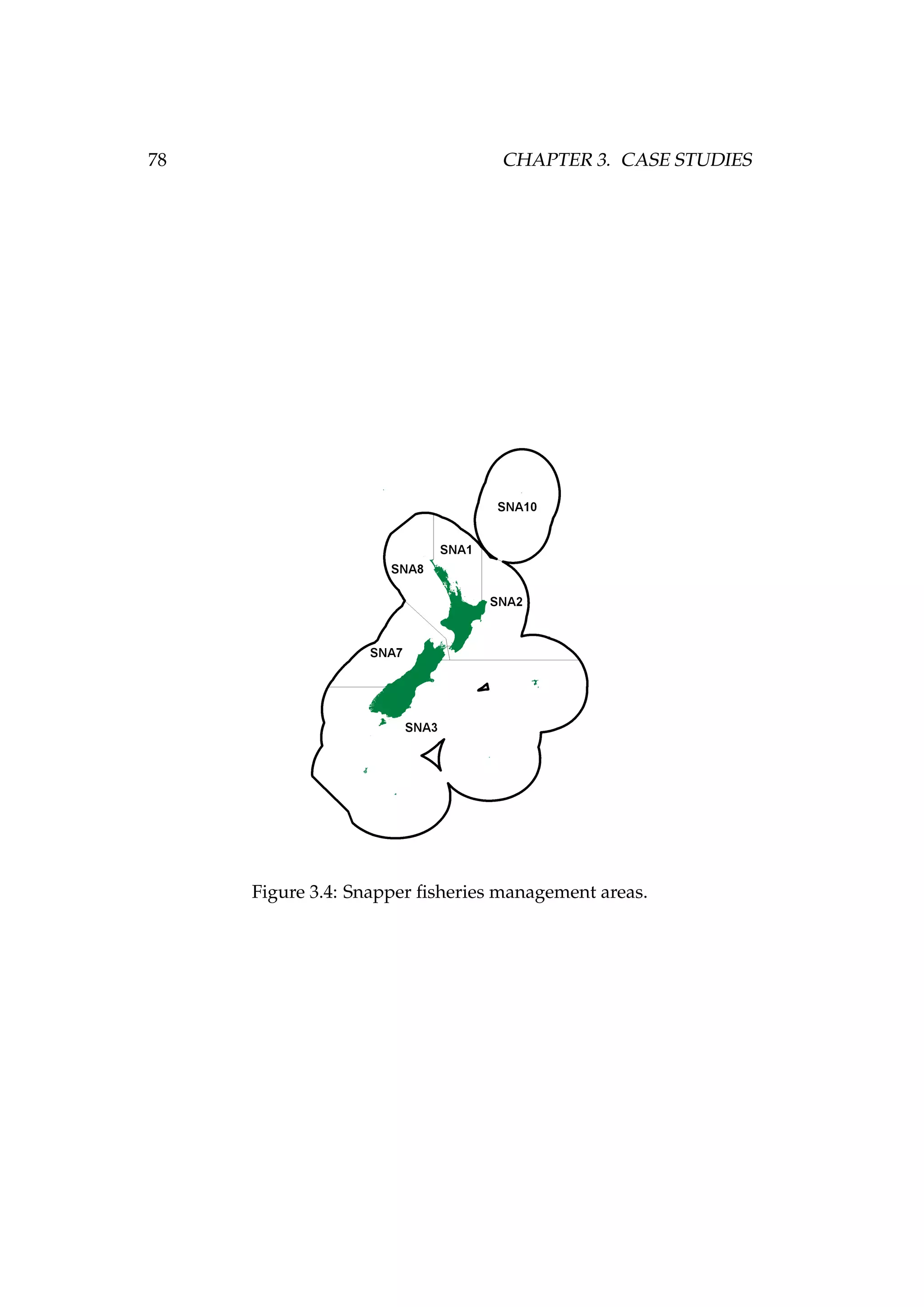
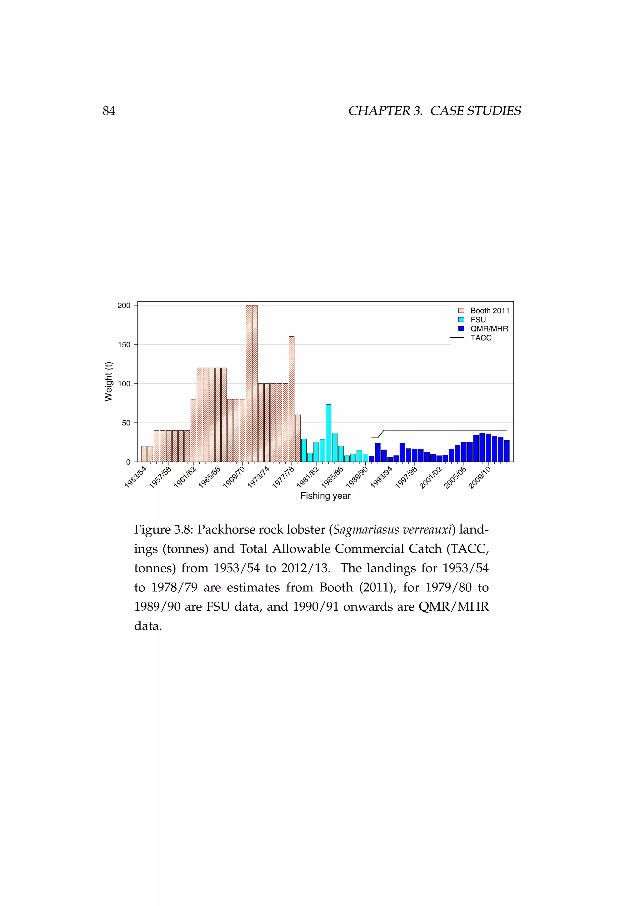
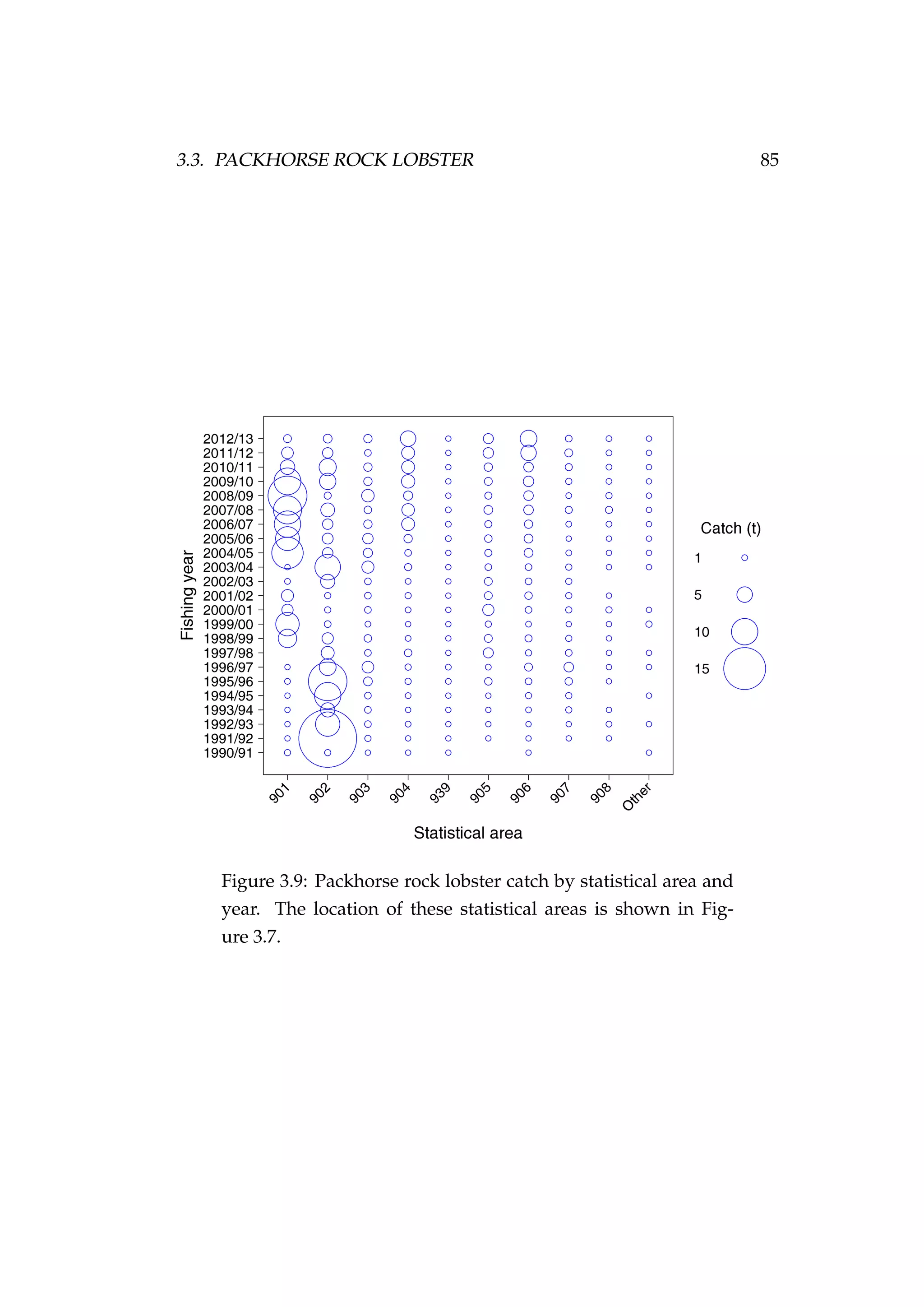
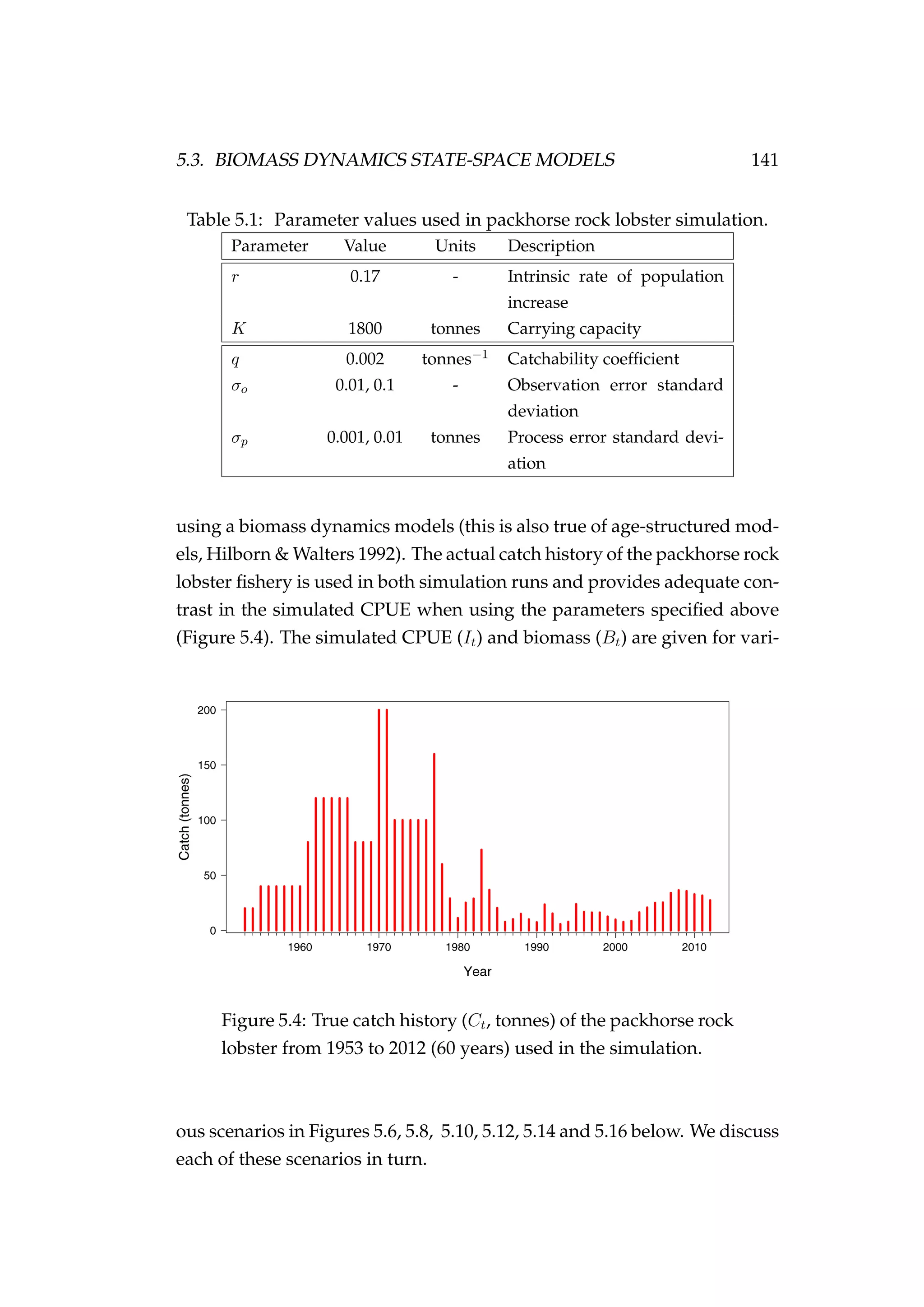
94. 82 CHAPTER 3. CASE STUDIES
Figure 3.7: Rock lobster fisheries management areas for the
packhorse rock lobster (Sagmariasus verreauxi) [top-left] and the
red rock lobster (Jasus edwardsii) [top-right], and the rock lob-
ster statistical areas in northern New Zealand within the CRA
1 and CRA 2 fisheries management areas [bottom].

95. 3.3. PACKHORSE ROCK LOBSTER 83
PHC is reported to be the largest species of rock lobster in the world, reach-
ing a total length of over half a metre and possibly weighing as much
as 18kg. PHC in Australia are known to grow faster than red rock lob-
sters here in New Zealand (Montgomery et al. 2009), but little is known
of the growth rates of packhorse in New Zealand. PHC in New Zealand
are thought to be the most migratory spiny lobster on Earth in terms of
proportions migrating and distance covered. They generally march north-
wards up the east coast of the North Island, the primary destination being
breeding grounds in the far north of the North Island. Little is known of
the timing or proportion of individuals that migrate northwards or what
they do once they reach their destination and breed. The size at onset of
breeding is large in females at about 160mm carapace-length (Booth 1984).
Typical of many other rock lobster species, females and males move sea-
sonally inshore and off as they respectively moult and reproduce.
Packhorse rock lobsters were amalgamated into the QMS on 1 April 1990
and the fishery is currently managed as a single QMA (PHC 1, Figure 3.7)
by MPI. Initially the TACC was set at 27 tonnes. This was raised in the
same year to 30.5 tonnes due to quota appeals (Ministry for Primary In-
dustries 2014b). The TACC remained at 30.5 tonnes for just two years
and was increased to 40.3 tonnes during the 1992/93 fishing year where it
has remained since. Since the introduction of the QMS, packhorse catches
have been relatively low and have only begun to approach the TACC in
the last five years (Figure 3.8). Historically landings were much higher
(Kensler & Skrzynski 1970, Booth 2011, Figure 3.8). While PHC 1 covers
New Zealand’s entire Exclusive Economic Zone (EEZ, Figure 3.7), PHC
are caught mainly in the north of the North Island (Figure 3.9).
Prior to the QMS, the PHC fishery was managed using input controls, in-
cluding: minimum legal size (MLS) regulations; a prohibition on taking
berried females (i.e. carrying external eggs) and soft shell lobsters; mak-
ing it illegal to commercially dive for or spear them; requiring pots to have
gaps or mesh large enough to allow small lobsters to escape; requiring that
they are landed ashore alive; and some local area closures. Today, all of
these input controls still remain.

96. 84 CHAPTER 3. CASE STUDIES
Figure 3.8: Packhorse rock lobster (Sagmariasus verreauxi) land-
ings (tonnes) and Total Allowable Commercial Catch (TACC,
tonnes) from 1953/54 to 2012/13. The landings for 1953/54
to 1978/79 are estimates from Booth (2011), for 1979/80 to
1989/90 are FSU data, and 1990/91 onwards are QMR/MHR
data.

97. 3.3. PACKHORSE ROCK LOBSTER 85
Figure 3.9: Packhorse rock lobster catch by statistical area and
year. The location of these statistical areas is shown in Fig-
ure 3.7.

98. 86 CHAPTER 3. CASE STUDIES
Fishers targeting PHC generally use different methods to those targeting
CRA. Generally longer soak times and more bait are used (this is also
the case in the Australian fisheries for PHC). Larger pots are also com-
mon when targeting the species, often due to strong tidal currents and the
sandy substrate on which they are set.
Recreational fishers may gather PHC by pot or hand (freediving or scuba)
but are subject to most of the other input controls in place for commercial
fishers. Recreational fishers may not take soft shell individuals or berried
females, and it is illegal to spear them. Additionally, a bag limit of 6 rock
lobsters (CRA and PHC combined) applies to recreational fishers. The
total recreational and customary catches for PHC are unknown.
The MLS of PHC for commercial and recreational fishers is 216mm tail-
length for both sexes. In many fish stocks a MLS is put in place to allow
most females to breed at least once before becoming legal to harvest. The
current MLS of PHC is smaller than the size at which 50% of females reach
maturity (Booth 1984). In comparison, the MLS in Australia is 104mm
carapace-length, much smaller than New Zealand where for females it is
equivalent to 155mm carapace-length. In Australia there is also a maxi-
mum legal size of 180mm carapace-length that is intended to look after
the stock of large breeders.
Two sources of information useful for stock assessment are available for
the packhorse rock lobsters in northern New Zealand. A catch history
and a catch per unit effort (CPUE) index. Catch data (QMR/MHR), from
1979/80 to 2012/13, were obtained from MPI. Historical catch estimates
were obtained from Booth (2011). The CPUE index and its development
is described in Webber (2013) and shown in Figure 3.10. The standardised
CPUE index is based on Catch Effort Landing Return (CELR) data from
1991/92 to 2012/13. The trend in the CPUE index shows a rise in catch
rates since the start of the series (Figure 3.10).
Some tag recapture and length-frequency data are also available for this
species but the sample sizes are very low. Only 12 lobsters have been
recaptured during the late 1970s and the number of individuals mea-
sured range from 6 to 508 from the 1990/91 to 2012/13 fishing years. The

99. 3.3. PACKHORSE ROCK LOBSTER 87
Figure 3.10: Standardised annual indices of CPUE (It) for log-
normal, binomial and combined models for packhorse rock
lobster Sagmariasus verreauxi (PHC) from 1991/92 to 2012/13.
The combined model is shown ± 2 s.e. All indices are scaled to
have a geometric mean of 1. Source: Webber (2013).
lack of these data and the limited knowledge on growth in PHC mean
that a length-structured stock assessment is currently not possible for this
species.
Packhorse rock lobster data are used in Chapter 5 as an example data set
for state-space biomass dynamics models. To fit properly, stock assess-
ment models require contrast in the catch history and/or CPUE indices.
The contrast in the catch history and CPUE series motivated the use of
PHC data as an example here.

100. 88 CHAPTER 3. CASE STUDIES

101. Chapter 4
An agent-based simulation model
In this chapter we describe an agent-based simulation model. Through-
out this chapter we use an example based on snapper in northern New
Zealand (Pagurus auratus, SNA 1, for more information on snapper see
Chapter 3, page 77) to illustrate how the model works. All of the variables
defined in this model are given in Table 4.1.
4.1 Introduction
Individuals are the building blocks of ecological systems. The properties
and behaviour of individuals determine the properties of the systems they
comprise. Population-level properties emerge from the interactions of in-
dividuals with each other and with their environment (Grimm & Rails-
back 2005) and variation among individuals is increasingly recognized as
fundamental to predictions about populations, communities, and ecosys-
tems (Smallegange & Coulson 2012).
Individual-based models (IBMs) and agent-based models (ABMs) de-
scribe populations in which individuals, or small groups of individuals
(super-individuals, Scheffer et al. 1995), differ in their growth, maturation,
movement, and mortality and follow these individuals through their life
history. They can be used to formulate theories about the behaviour of
89

102. 90 CHAPTER 4. AN AGENT-BASED SIMULATION MODEL
Table 4.1: List of model parameters. SD is the standard deviation.
Symbol Type Dimensions Description
f scalar 1 Index of fisheries f = {0, 1, . . . , F}
j scalar 1 Index of stocks j = {0, 1, . . . , J}
s scalar 1 Index of sexes
y scalar 1 Index of years y = {0, 1, . . . , Y }
z scalar 1 Index of areas z = {0, 1, . . . , Z}
R0, σR vector J + 1 Mean and SD of recruitment
h vector J + 1 Stock recruitment steepness
ρ vector J + 1 Recruitment autocorrelation
pmale vector J + 1 The proportion of recruits that are male
Ξ matrix J + 1 × Z + 1 The proportion of total recruitment from each
stock into each area
vector Z + 1 This defines the areas that make up a stock
µA50 , σA50 vector s Mean and SD of age at 50% maturity
µAto95 , σAto95 vector s Mean and SD of difference in age at 95% maturity
µL, σL vector s Maturity
µR, σR vector s Maturity
µL∞ , σL∞ vector s Mean and SD of asymptotic length (cm)
µk, σk vector s Brody growth coefficient (years−1)
t0 vector s Time at which length is zero (years)
c vector s Coefficient of variation of growth
µα, σα vector s Length-weight
µβ, σβ vector s Length-weight
µM , σM vector s Mean and SD of natural mortality (M)
µq, σq vector f Mean and SD of the catchability coefficient (q)
γ1 matrix s × f Double normal selectivity
γL matrix s × f Double normal selectivity
γR matrix s × f Double normal selectivity
Ω matrix Z + 1 × Z + 1 Migration matrix
ψ scalar 1 Probability of home switching
σo scalar 1 Observation error standard deviation

103. 4.1. INTRODUCTION 91
individuals. We can then test these theories by seeing how well they re-
produce patterns observed at the system level.
Despite being a very flexible modelling approach, the computational over-
heads of IBMs and ABMs can be very high. This can make some models
impractical, particularly if trying to estimate parameter values. However,
new hybrid methods that tie classical models with individual-based as-
pects (e.g. Gray et al. 2006) and some modern computational methods may
be the key to solving such dilemmas. The benefits of such approaches may
be worthwhile in some cases. In species or populations with few individu-
als (e.g. marine mammals), such models make sense if the data is available
as the computational overheads will be reasonably low and complex be-
havioral attributes may be incorporated. However, when modelling popu-
lations with many individuals (e.g. fish) then there must be a good reason
to do so using ABMs rather than age-structured models.
Classic statistical age-structured stock assessment models track cohorts of
fish though time and in some cases space. In a spatially explicit model,
a proportion of fish within each cohort may move between different ar-
eas within the model in a time step. When fish move from one area to
another, they are lumped together with other fish in the new area of the
same age (and/or sex/maturity) in the partition. This means that we no
longer know which fish came from where in the next time step. Now, con-
sider that these fish may be moving to a certain area to spawn, a common
occurrence in fish stocks. If these fish do move to a certain area to spawn,
will they return to the same general area they came from, or will they move
on to any suitable area within the model space? The former implies that
we must know the area from which the fish came from before embarking
on their spawning migration.
There is evidence in some fish populations (e.g. Antarctic toothfish and
New Zealand snapper, see Chapter 3, pages 73 and 77) that individuals
may return to the area that they originally came from, a phenomenon
known as site or home fidelity. If site fidelity is operating within a popula-
tion, then this will inflate the recapture probabilities of individuals within
a population in tag-recapture experiments (resulting in the model under-

104. 92 CHAPTER 4. AN AGENT-BASED SIMULATION MODEL
estimating population size). To account for this, it may be necessary to
track tagged fish as individuals, or agents, and store information on their
home site which would adjust our recapture probabilities. Site or home fi-
delity could also affect other processes such as the spawning stock biomass
(SSB) of a population. For example, if all fish return home to spawn then
the SSB in the home area could be different than if fish simply stayed
where they were to spawn. To test these ideas, a fish population could be
simulated in a way that the individuals (or groups of individuals) within
the population display site fidelity.
This chapter describes a spatially explicit multi-generational agent-
structured fish simulation model that allows flexibility in specifying popu-
lation and spatial dynamics. The model has the potential to consider indi-
vidual variability, individual movement, and spatial heterogeneity in the
environment. The aim is to construct a model that is sufficiently rich that
it can be used to simulate complete, realistic fish populations. The simu-
lated data can be used to test stock assessment methodologies - which are
usually based on samples from the population, and incomplete data.
4.2 The agent
This model was developed to track agents which are collections of individ-
ual fish. The advantage of an agent based model is that all fish in an agent
have identical properties, and can therefore be treated simultaneously. An
agent can contain a single fish (individual-based), any number of fish, or
an entire cohort of fish (all fish of the same age in the population). Each
agent i contains all of the attributes of the fish in that agent. The attributes
of an agent include how many individuals an agent contains fi, biological
information such as the age (ai), sex (si), length ( i), and maturity (mi) and
information on the location of agents (zi), the home site of the fish in the
agent (hi) if the fish in the agent are tagged or not (ti), and the year that
the fish was tagged (yi) (Table 4.2). The areas in the model are labelled as
z = 0, . . . , Z where Z + 1 is the total number of areas in the model. The
years in the model, after initialisation, are labelled as y = 0, . . . , Y where

105. 4.2. THE AGENT 93
Y + 1 is the total number of years. Agents also store a set of parameters
Table 4.2: The attributes of an agent i including how many in-
dividuals an agent contains (fi), biological information such as
the age (ai), sex (si), length ( i), and maturity (mi) and informa-
tion on the location of agents (zi), the home site of the fish in
the agent (hi) if the fish in the agent are tagged or not (ti), and
the year that the fish received a tag (yi). The number of areas
in the model is Z + 1 and the number of years in the model
is Y + 1. Agents also store parameters specific to that agent
including growth parameters (L∞,i and ki), length-weight (αi
and βi), maturity (A50,i, Ato95,i, Li and Ri) and natural mortality
(Mi).
Attribute Symbol C++ type Possible values
Frequency fi int 0 ≤ fi ≤ Fmax
Age ai int amin ≤ ai ≤ ∞
Sex si bool 0, 1
Length i double -
Maturity mi bool 0, 1
Location zi int 0 ≤ zi ≤ Z
Home hi int 0 ≤ hi ≤ Z
Tagged ti int −1 ≤ ti ≤ Z
Tag year yi int −1 ≤ yi ≤ Y
Length L∞,i double -
Length ki double -
Length-weight αi double -
Length-weight βi double -
Maturity A50,i double -
Maturity Ato95,i double -
Maturity Li double -
Maturity Ri double -
Natural mortality Mi double -
specific to the fish in that agent, and a set of pointers to other agents in the
population. These pointers are further described in Section 4.2.1 below.
Agents are created via recruitment or if an already extant agent splits. At

106. 94 CHAPTER 4. AN AGENT-BASED SIMULATION MODEL
recruitment the value of some agent attributes are set to −1 (i.e. ti = −1
and yi = −1), this simply indicates that the agent has not been tagged
yet and helps differentiate between an agent tagged in location zi = 0 or
during year yi = 0. Agents can move randomly via migration or deter-
ministically via home fidelity. Agents are either merged when they get too
small or destroyed when an agent becomes depleted to fi = 0 through
natural mortality, fishing and/or splitting (see Section 4.2.4, page 102).
4.2.1 Accessing agents
In this model the population is made up of a collection of agents. The
agents are placed in sequences ordered by unique paths (mapped by sets
of pointers) that can be used to traverse sequences of agents. One path
traverses the entire population and is used to sequentially access all of the
agents in the population and modify the content of each agent along the
way (e.g. applying natural mortality) or gather information about the pop-
ulation (e.g. summing up the weight of all of the individuals in the popula-
tion to get the biomass). We represent this sequence of agents graphically
as
Pointer
null
i = 1
next
prev
i = 2
next
prev
· · ·
· · ·
i = n
next
prev
null
where each of the boxes represent a single agent containing all of the in-
formation outlined in Table 4.2 as well as the pointers used to traverse the
sequence. The first agent in the sequence is accessed using a stored pointer
to that agent (represented as “Pointer” here). The arrows represent point-
ers to other agents in the sequence, these can point to the next (“next”)
agent or the previous (“prev”) agent in a sequence. The last agent in the
sequence of agents points next to “null”. Thus, traversing a sequence of
agents in the code is stopped once the pointer to the next agent becomes
null. Similarly, the first agent in a sequence points backwards to null. We
simplify this diagram to

107. 4.2. THE AGENT 95
Pointer
n
n
where the “n” represents “null”. Other paths exist that access the agents
by age and by location. The population can be traversed by whichever
path is most relevant for the operations at hand. This is also useful as
tasks can be passed off as different threads by age or by area. On a multi-
core computer this can improve the time the model takes to run. For ex-
ample, the biomass can be summed up by area as different threads, then
the separate results for each area can be summed to get the total biomass.
Graphical representations of the age- and area-sequences are shown be-
low. These sequences are accessed by storing a vector of pointers to the
first age or area in a sequence.
Age pointer
1
2
...
A
n
n
n
n
n
n
Area pointer
0
1
2
n
n
n
n
n
n
Arranging the population of agents as strings of objects connected by
pointers, rather than a set of matrices and vectors holding all of the infor-
mation about the population, is done to reduce the memory requirements
of the model. A model structured in the standard way, using matrices and
vectors, requires that memory be allocated for the entire object (matrix or
vector) even if many of the values within that object are unused (i.e. zero
fish are associated with many values in each object). This model only al-

108. 96 CHAPTER 4. AN AGENT-BASED SIMULATION MODEL
locates memory if there are fish within an agent, otherwise that agent is
destroyed and the memory for that agent freed.
4.2.2 Creating agents
New agents are created by recruitment (or splitting agents, Section 4.2.4,
page 102). When an agent recruits to a population it is added to the begin-
ning of the minimum age sequence. In doing so, several pointers require
redirection shown graphically below
Age pointer
1
2
...
A
n
n
n
n
n
n
where the new agent is green, as are the redirected pointers.
When a new agent is created via recruitment that agent requires initialisa-
tion with agent specific parameter values, age, sex, length, location and so
on. The values these variables take are described below.
Agent-specific parameters
Several parameters are allocated to agents when they are recruited to
the population including parameters relating to growth (L∞,i and ki), the
length-weight relationship (αi and βi), maturity (A50,i, Ato95,i, Li and Ri)
and natural mortality (Mi). In the model, each of these parameters have
their own mean and standard deviation. When an agent is created the
value of each of these parameters for each agent is drawn from a normal
distribution (e.g. Figure 4.1). The parameter t0 is not stored within an
agent because it is only required at the time the agent is created (see Ta-
ble 4.1 and Section 4.2.2 above).

109. 4.2. THE AGENT 97
Figure 4.1: Frequency histograms of the parameters allocated
to agents upon their creation. The values plotted are from the
population after initialisation but before fishing begins (i.e. the
end of phase 2).

110. 98 CHAPTER 4. AN AGENT-BASED SIMULATION MODEL
Frequency (fi = {0, 1, . . . , Fmax})
The frequency or number of individuals contained in an agent is specified
at recruitment. This is further described in Section 4.4.5, page 115.
Age (ai = {amin, . . . , A})
The age of recruited individuals within each agent is
ai = amin,
where amin is the specified minimum age (years) within the model. For
more information see Chapter 1, page 17. Ageing is described later in this
chapter in Section 4.4.1, page 110.
Sex (si = {0, 1})
All of the individuals within an agent are either female (si = 0) or male
(si = 1). Sex is randomly allocated at recruitment using a binomial dis-
tribution (Equation 4.17). The sex of all individuals within an agent is
determined at recruitment and does not change. The model may be run as
a single sex model. For more information see Chapter 1, page 18.
Length ( i)
Growth in the model can be either deterministic or stochastic. If growth is
set to be deterministic then the initial length i of recruits within agent i is
equal to the mean length µ ,i of a fish at amin in agent i. This is determined
using the von Bertalanffy growth function
µ ,i = L∞,i 1 − e−ki(amin−t0)
, (4.1)
where L∞,i, ki, and t0 are the parameters of the von Bertalanffy growth
function (see Chapter 1, page 19). L∞,i and ki are agent specific parame-
ters, t0 is not. If growth is set to be stochastic then the initial length of new

111. 4.2. THE AGENT 99
recruits is drawn randomly from a normal distribution
i ∼ N µ ,i, σ2
where σ = c µ ,i, (4.2)
and c is the coefficient of variation of growth (e.g. Figure 4.2). Growth is
described later in this chapter in Section 4.4.2, page 110.
Figure 4.2: The initial length (cm) of females [left] and males
[right] allocated to agents during initialisation.
Maturity (mi = {0, 1})
All of the individuals within an agent are either immature (mi = 0) or
mature (mi = 1). At recruitment, all agents are immature. For more in-
formation see Chapter 1, page 21. Maturation is described later in this
chapter in Section 4.4.3, page 112.
Location (zi = {0, 1, . . . , Z})
A multinomial distribution is used to determine the recruitment location
z using a z × 1 stock definition vector and a (J + 1) × (Z + 1) recruit-
ment matrix Ξ that defines the proportion of stock j recruiting to area z.

112. 100 CHAPTER 4. AN AGENT-BASED SIMULATION MODEL
The stock definition vector simply specifies which areas belong to which
stocks. The number of stocks cannot exceed the number of areas. For ex-
ample, a three stock, three area model would be specified as = {0, 1, 2}.
A three area, two stock model in which the first two areas make up the
first stock would be = {0, 0, 1}. The recruitment matrix defines the pro-
portion of each stock’s recruits that recruit to each area in the model. For
example, a three stock, three area model where all recruitment from each
stock j is to each area z would be defined using
Ξ =



1 0 0
0 1 0
0 0 1


 ,
where all rows sum to one. A three area, two stock model where recruit-
ment from the first stock is into the first area and recruitment from the
second stock is into the remaining two areas would be defined using
Ξ =



1 0
0 0.5
0 0.5


 .
A three area, one stock model is defined as
Ξ =



1
3
1
3
1
3


 .
Alternatively, one could specify a three area, three stock model where re-
cruits from different stocks “leak” into different areas
Ξ =



0.7 0.2 0.1
0.2 0.6 0.2
0.1 0.2 0.7



where z Ξz,j = 1 ∀ stocks j. Migration is described later in this chapter
in Section 4.4.7, page 117. For more information on stocks and areas see
Chapter 1, page 31.

113. 4.2. THE AGENT 101
Home (hi = {0, 1, . . . , Z})
The home site is defined as the area or cell that the agent recruited to. The
parameter ψ defines the probability of an agent switching its home site to
its current location at a particular time step. If the probability of switching
is low, then agents will rarely switch their home site, if the probability is
high, then agents will switch their home site often. If ψ = 0 then agents
will never switch their home site, if ψ = 1 then agents will essentially
follow a random walk. The only way for a fish to pick a home site is if
they have visited that cell. This structure implements the behaviours of a
random walk versus attraction to an area.
Tagged and tag year (ti = {−1, 0, . . . , Z} and yi = {−1, 0, . . . , Y })
All of the individuals within an agent are either untagged (ti = −1) or
tagged (ti = z) where z is the cell that the fish was tagged in. At re-
cruitment no fish are tagged. Similarly, no fish have a tag year at recruit-
ment (yi = −1). Tagging is described later in this chapter in Section 4.4.9,
page 122.
4.2.3 Deleting agents
If an agent becomes depleted (by natural or fishing mortality) so that no
more individuals are contained in that agent (fi = 0) then the agent is
removed from the population, the memory for that agent is freed, and
all pointers pointing to that agent are appropriately redirected. We pro-
vide some examples below of an agent being deleted from the end of a
sequence, from the end of an age sequence, and from the middle of an
area sequence. In these examples, the deleted agent is shown in red with
a cross and the redirected pointers in red. The old pointers are shown in
grey.
Pointer
n
n

114. 102 CHAPTER 4. AN AGENT-BASED SIMULATION MODEL
Age pointer
1
2
...
A
n
n
n
n
n
n
Area pointer
0
1
2
n
n
n
n
n
n
4.2.4 Splitting agents
Some processes require agents to split into two or more different agents.
These process include maturation, migration, and tag-release events. For
example, if an individual within an agent is tagged and released, this indi-
vidual splits from its parent agent into its own agent and all the attributes
of the parent agent are copied into the new agent except for the tag status.
Or, if a portion of the individuals within an agent migrate to another loca-
tion, those individuals split from the parent agent to form their own agent
in the new location. For example, if the agent shown in green below was
to split
Pointer
n
n
the agent pointer sequence would become
Pointer
n
n
If the agent being split is moved to a different area the area sequence
would become

115. 4.2. THE AGENT 103
Area pointer
0
1
2
n
n
n
n
n
n
n
4.2.5 Moving agents
If an agent is moved from the start of a sequence then the array of pointers
by area must be redirected to point to the next agent, and the next agents
backwards pointer must be set to null. The agent being moved is then set
as the first agent in the new area sequence, and all pointers must be redi-
rected as appropriate. In the diagram below, all pointers being redirected
are shown in red, the old pointers are grey, and the agent being moved is
red.
Area pointer
0
1
2
n
n
n
n
n
n
n
If an agent is being moved from the middle of a sequence

116. 104 CHAPTER 4. AN AGENT-BASED SIMULATION MODEL
Area pointer
0
1
2
n
n
n
n
n
n
n
If an agent is being moved from the end of a sequence
Area pointer
0
1
2
n
n
n
n
n
n
n
If an agent is being moved from the start and end of a sequence
Area pointer
0
1
2
n
n
n
n
n
n
n
If an agent moves to the start and end of a sequence

117. 4.2. THE AGENT 105
Area pointer
0
1
2
n
n
n
n
n
n
4.2.6 Merging agents
When an agent represents a school or group rather than an individual, for
computational efficiency (and in some cases for biological plausibility) it is
necessary to merge significantly depleted agents (this would be analogous
to schools merging). If the number of individuals within an agent (fi) is
equal to or less than the user specified merge threshold (Fmin), then that
agent (i1) is selected for merging. The program then searches for another
agent in the population that is suitable for merging with the selected agent.
If another agent (i2) is found with sufficiently depleted individuals, then
the two agents must meet a set of criteria for merging to occur. Agents will
only merge if they are the same age (ai1 = ai2 ), same sex (si1 = si2 ), in the
same location (zi1 = zi2 ), from the same home site (hi1 = hi2 ), are the same
maturity (mi1 = mi2 ), have the same tag status (ti1 = ti2 ) and were tagged
in the same year (yi1 = yi2 ), and the sum of the fish frequencies merging
agents will not be greater than the maximum agent size (fi ≤ Fmax). The
merging of the two agents then involves combining the individuals and
finding the weighted mean length and weighted mean parameter values

118. 106 CHAPTER 4. AN AGENT-BASED SIMULATION MODEL
of the individuals in the agents.
fi = fi1 + fi2 if



fi1 ≤ Fmin
fi2 ≤ Fmin
fi ≤ Fmax
ai1 = ai2 age
hi1 = hi2 home
mi1 = mi2 maturity
si1 = si2 sex
ti1 = ti2 tag
yi1 = yi2 tag year
zi1 = zi2 location
, (4.3)
where fi is the number of individual fish represented by the merged agent.
The weighted mean length and weighted mean parameter values (e.g. L∞,
k, M, etc) are found using
θi =
i∈{i1,i2} fiθi
fi
, (4.4)
where θi is the length or parameter value before merging and θi is the
weighted mean length or parameter value. This is a computationally ex-
pensive exercise so has been developed to work on multi-core computers
(multi-threading) by spawning a thread for each age group or cell and
running the algorithm on each simultaneously.
Care must be taken if allowing the merging of agents. If merging is al-
lowed in a model run then the merging process (specifically taking the
weighted mean of the length or parameter values) can dilute the individ-
ual nature of the model such that the model will begin to behave more
like an age-structured model. For example, the length of an agent will ap-
proach the mean length within the population (for a given cohort) as more
and more agents are merged. The parameter Fmin can be used to reduce
the merging issue (i.e. setting a lower Fmin will prevent too much merging
at a computational cost).

119. 4.3. MODEL STRUCTURE 107
4.3 Model structure
The main body of the model is structured in two parts: initialisation and
application of the fishery.
4.3.1 Initialisation
Initialisation is done in two phases. The first phase recruits R0,j individ-
uals into each stock (j) in the population each year until an equilibrium
age-structure is achieved. During each year the following sequence is fol-
lowed:
1. Ageing
2. Growth
3. Maturation
4. Recruitment
5. Spawning
6. Natural mortality
The details of each of these processes is described in Section 4.4. The pop-
ulation is initialised over many years until the population reaches equilib-
rium age-structure and the spawning stock biomass stabilises in each stock
(Figure 4.3). Phase 2 then follows wherein random variation is introduced
into the recruitment and migration is allowed:
1. Ageing
2. Growth
3. Maturation
4. Migrate home (new step)
5. Recruitment
6. Spawning

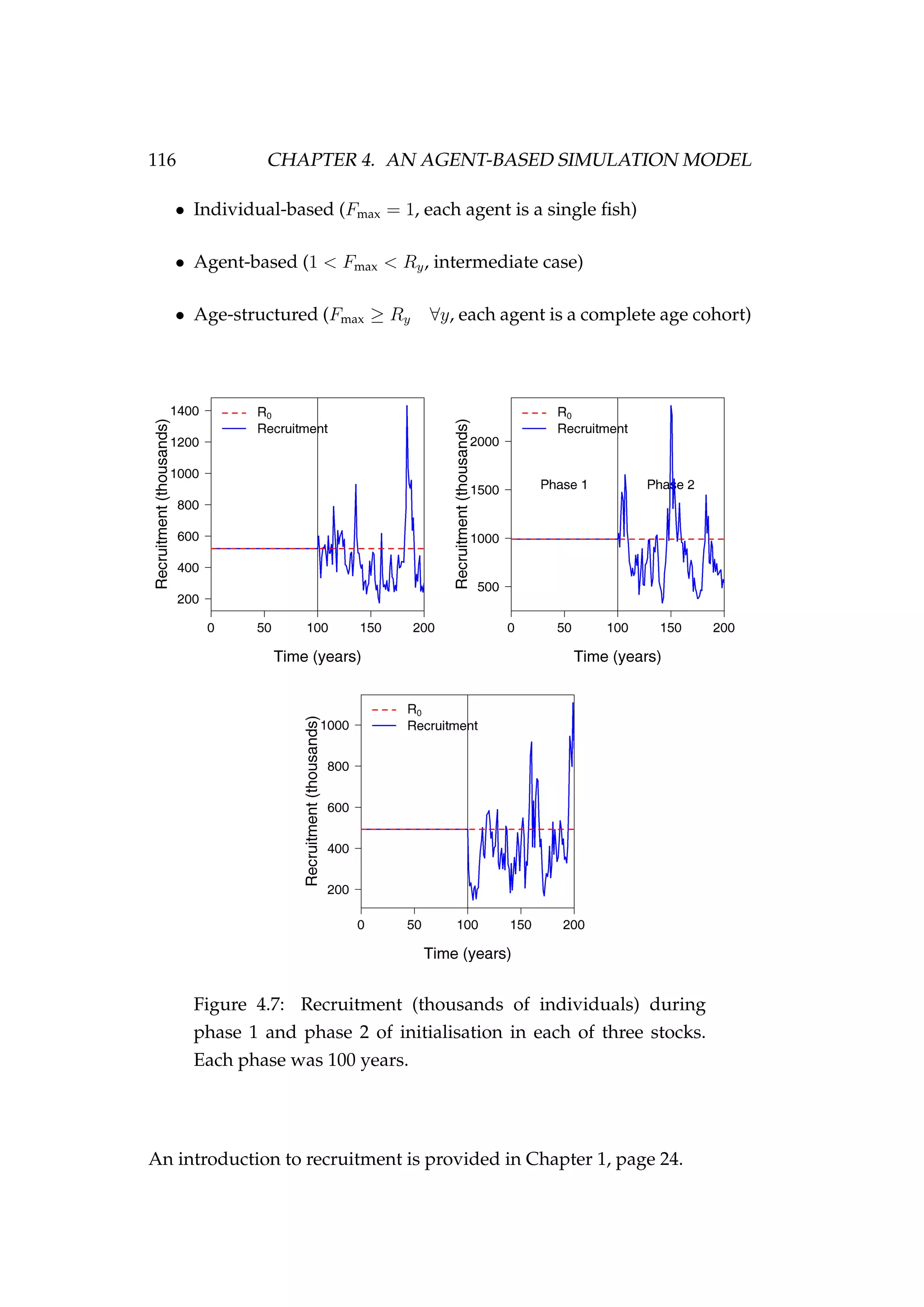
120. 108 CHAPTER 4. AN AGENT-BASED SIMULATION MODEL
7. Migration (new step)
8. Natural mortality
In our example, we have specified phase 1 and phase 2 to both be 100 years
(Figure 4.3).
Figure 4.3: Numbers at age in the population at the end of
phase 2 compared to the non-stochastic equilibrium numbers
at age [top left] and the spawning stock biomass (tonnes) of
each of three stocks during phase 1 and phase 2.

121. 4.4. PROCESSES 109
4.3.2 Applying the fishery
The annual cycle during the years that the fishery operates includes the
following processes:
1. Ageing
2. Growth
3. Maturation
4. Migrate home
5. Recruitment
6. Spawning
7. Tagging (new step)
8. Migration
9. Natural mortality and fishing mortality (new step)
There are switches between deterministic and stochastic settings for some
of these processes. These may be used to allow a user to explore differ-
ences between these approaches and the influence of variability on model
outcomes. Each year is split up into time-steps so that some processes
may be split between multiple time steps (e.g. applying half of the natural
mortality before calculating the spawning stock biomass).
4.4 Processes
Processes in the model include
1. Ageing (deterministic)
2. Growth (deterministic or stochastic)
3. Maturation (stochastic)
4. Spawning (deterministic)
5. Recruitment (stochastic)

122. 110 CHAPTER 4. AN AGENT-BASED SIMULATION MODEL
6. Natural mortality (stochastic)
7. Fishing mortality (stochastic)
8. Tagging (stochastic)
9. Migration home (deterministic)
10. Migration (stochastic)
We now describe each of these processes in detail.
4.4.1 Ageing
During ageing, all agents are aged by one year
ai = ai + 1, (4.5)
where ai is the age of fish in agent i before ageing and ai is the age of
fish after ageing. There is no limit on the age a fish can reach in the model.
This means that the fish in an agent could reach a very old age (much older
than is possible). We accept that, biologically, this is not possible, however,
very few of these old agents will persist in the modelled population so we
ignore this problem. When presenting these data we deal with these very
old fish by simply amalgamating them into a plus group (see Chapter 1,
page 17).
4.4.2 Growth
Using the von Bertalanffy growth parameters (L∞,i and ki) for agent i, the
expected annual growth increment (∆¯i) for an agent of length i is
∆¯i =



(L∞,i − i)(1 − e−ki
) if i ≤ L∞,i
0 if i > L∞,i
. (4.6)
If growth is set to be deterministic then ∆¯i is the growth increment for
agent i in that year and the new length of the agent after growth i is
i = i + ∆¯i. (4.7)

123. 4.4. PROCESSES 111
If growth is set to be stochastic then the growth increment is simulated
as a normally distributed random variable with mean ∆¯i and standard
deviation σ∆
∆ i ∼ N ∆¯i, σ2
∆ where σ∆ i
= c ∆¯i, (4.8)
∆ i is the simulated growth increment to be added to the length of the
individuals in agent i and c is the coefficient of variation of growth. The
new length of the agent after growth i is
i = i + ∆ i. (4.9)
An example is given in Figure 4.4. Growth in fisheries models is intro-
Figure 4.4: Distributions of length (cm) at age (years) of females
[left] and males [right] of agents in the initialised population.
duced in Chapter 1, page 19.

124. 112 CHAPTER 4. AN AGENT-BASED SIMULATION MODEL
4.4.3 Maturation
A logistic producing ogive is used to describe the proportion of fish in the
population that are mature in any given year
µm,i =



0 if xi < Li
λ(Li) if xi = Li
(λ(xi) − λ(xi − 1))/(1 − λ(xi − 1)) if Li < xi < Hi
1 if xi ≥ Hi
, (4.10)
where
λ(xi) = 1 1 + 19(A50,i−x)/Ato95,i
,
µm,i represents the probability a fish of size xi (where xi could be age ai,
length i, or weight wi) will become mature in agent i. The parameters Li
and Hi respectively define the x at which no fish are mature and the xi
at which all fish are mature, respectively. A50,i and Ato95,i are respectively
the xi at which 50% of individuals within the population are mature and
the difference in xi at which 95% of individuals within the population are
mature. The number of fish within the agent that mature is a draw from a
binomial distribution
mi ∼ Bin(fi, µm,i), (4.11)
If a non zero subset of individuals within the agent reach maturity, then
these individuals will split from the parent agent and form their own new
agent, leaving the as yet immature individuals behind (e.g. Figure 4.5).
Maturation is covered in more detail in Chapter 1, page 21.
4.4.4 Spawning
Spawning refers to the time at which the spawning stock biomass SSBy
and stock recruitment relationship SR(SSBy) are calculated. The spawn-
ing stock biomass is calculated as
SSBy =
Iy
i=1
fi,ywi,ymi,y, (4.12)

125. 4.4. PROCESSES 113
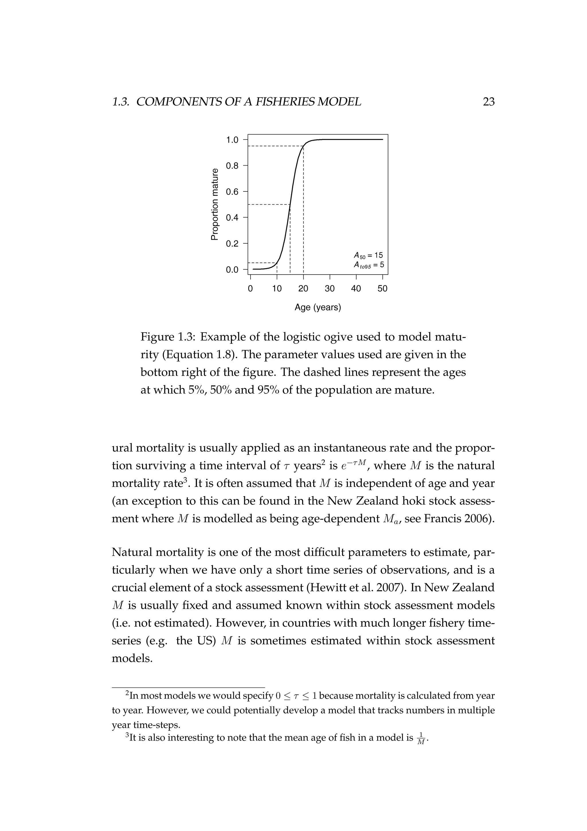
Figure 4.5: The proportion of fish mature by age (years) in
the initialised population for females [top left] and males [top
right] showing the deterministic maturity ogive (Numerical),
and the proportion of mature female and male fish by length
(cm) [bottom]. The black lines sit directly behind the red lines.

126. 114 CHAPTER 4. AN AGENT-BASED SIMULATION MODEL
where wi,y is the weight (tonnes) of agent i during year y calculated as
wi = αi
βi
i . (4.13)
Calculating the total weight of agent i also allows comparisons between
length and weight, and age and weight to be made (Figure 4.6).
Figure 4.6: The length-weight relationship [left] and the age-
weight relationship [right].
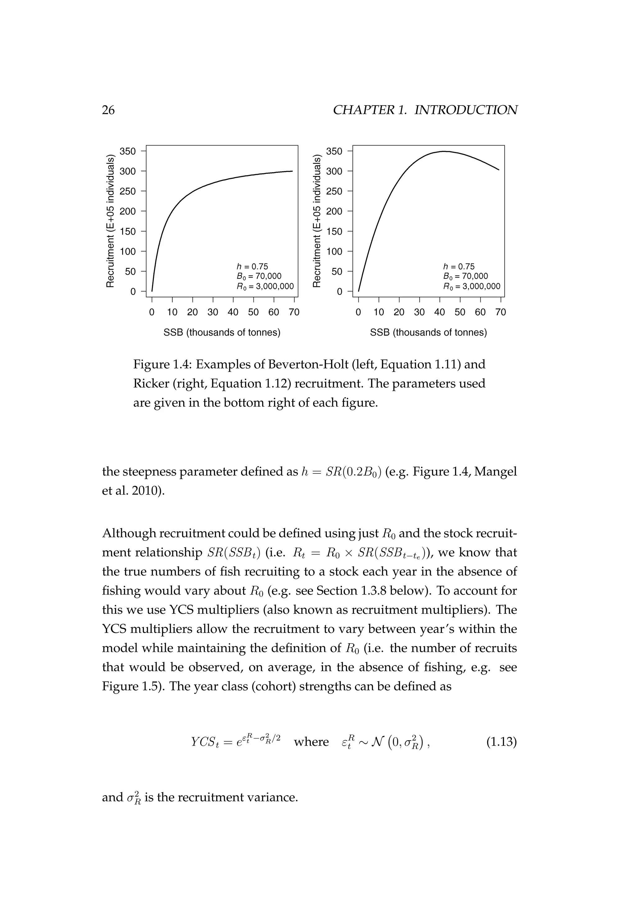
A Beverton-Holt stock recruitment relationship is used
SR(SSBy) =
SSBy
B0
1 −
5h − 1
4h
1 −
SSBy
B0
, (4.14)
where B0 is the deterministic virgin biomass (tonnes) and h is the steep-
ness parameter. For more information on spawning stock biomass see
Chapter 1, page 24. For more information on stock recruitment see Chap-
ter 1, page 24.
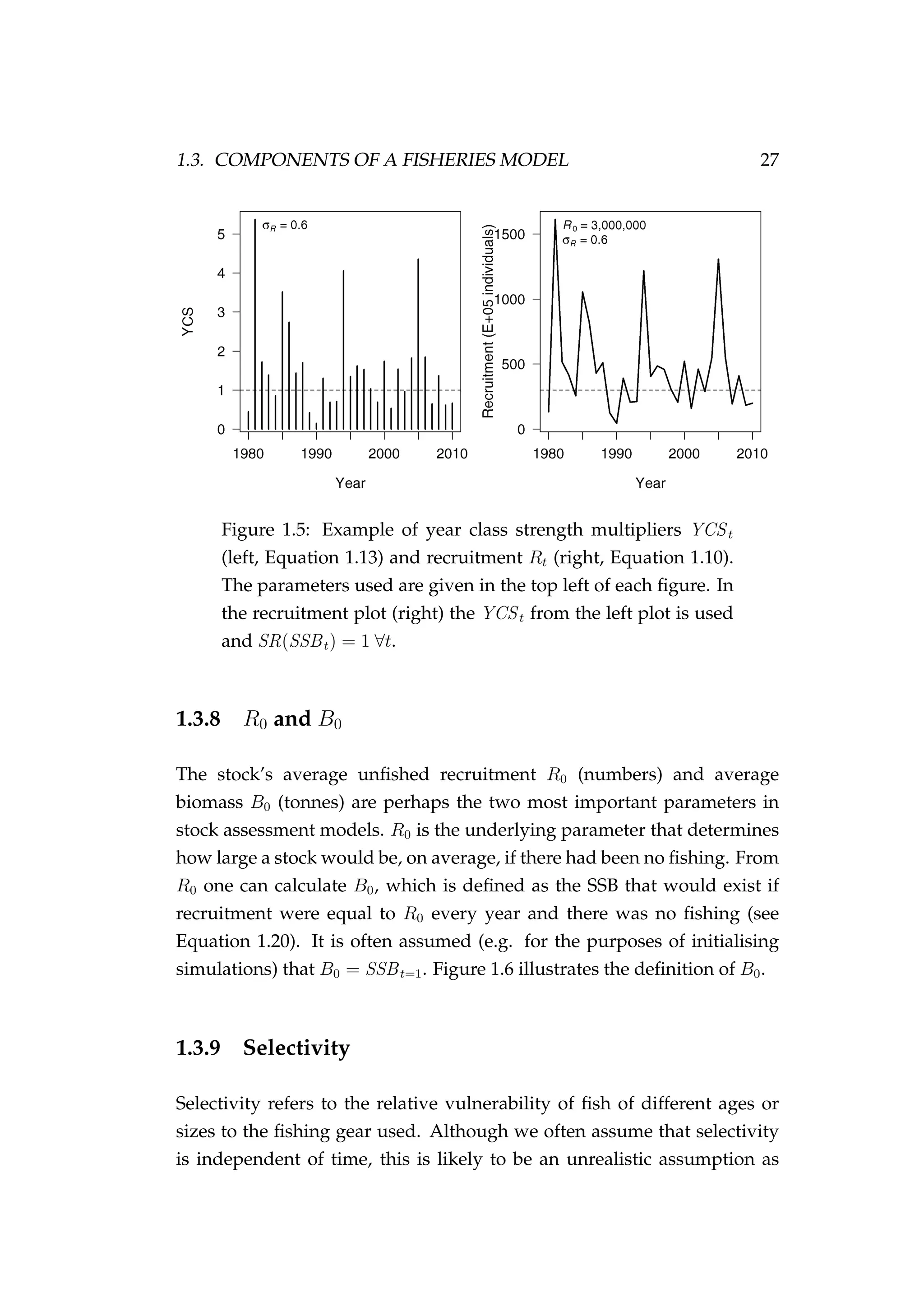
4.4.5 Recruitment
Recruitment involves the addition of new individuals and thus new agents
to the population each year. The number of individual fish that recruit in

127. 4.4. PROCESSES 115
year y is assumed to be dependent on an underlying average recruitment
(R0), the spawning stock biomass during the previous year (y − 1), and
the strength of the year class (cohort) during year y. During phase two
of initialisation, the recruitment for each year is modified by log-normal
annual deviations and the stock recruitment relationship
Ry = R0 × SR(SSBy−1) × eεR
y −σ2
ε /2
, (4.15)
where
εR
y =
√
ρεR
y−1 + 1 − ρεy and εy ∼ N 0, σ2
ε ,
σε is the standard deviation of εy, and ρ determines the serial auto-
correlation in recruitment between years. The total number of recruits Ry
in year y is then split by location and sex using Equations 4.16 and 4.17
below
Ry,z ∼ Multinomial (Ry, ξ1, . . . , ξZ) , (4.16)
where Ry,z is the number of individuals recruiting to location z in year y
and ξ1, . . . , ξZ is a column of Ξ specifying the probabilities of recruiting in
location z (see Section 4.2.2, page 99). Ry,z is then passed to
Rs,y,z ∼ B(Ry,z, pmale), (4.17)
where Rs,y,z is the number of individuals recruiting as sex s, to location z,
in year y, and pmale is the is the probability that a fish will be male (i.e. si =
1). These individual fish are then allocated into agent structures where the
maximum number of individuals contained in an agent is Fmax
fi,y = Fmax where
Iamin,y
i=1
fi,y = Ry ∀y, (4.18)
Iamin,y is the number of agents in a cohort in year y which is determined by
Iamin,y =
Ry
Fmax
. (4.19)
If Ry/Fmax is not a whole number in year y, then the remaining fIamin,y
individuals are placed in agent Iamin,y so that
Iamin,y
i=1 fi,y = Ry is true for
that year (i.e. we create Iamin,y − 1 agents of full size Fmax and one of size
Ry − (Iamin,y − 1)Fmax). The following values of Fmax can be supplied to
structure the model as an individual-based model, agent-based model, or
age-structured model:

128. 116 CHAPTER 4. AN AGENT-BASED SIMULATION MODEL
• Individual-based (Fmax = 1, each agent is a single fish)
• Agent-based (1 < Fmax < Ry, intermediate case)
• Age-structured (Fmax ≥ Ry ∀y, each agent is a complete age cohort)
Figure 4.7: Recruitment (thousands of individuals) during
phase 1 and phase 2 of initialisation in each of three stocks.
Each phase was 100 years.
An introduction to recruitment is provided in Chapter 1, page 24.

129. 4.4. PROCESSES 117
4.4.6 Natural mortality
Natural mortality is the death of fish due to causes not associated with
fishing (e.g. cannibalism, competition, disease, old age, predation). Nat-
ural mortality is applied to the frequency of individuals within agents fi
using a binomial distribution
fi ∼ Bin fi, e−τMi
, (4.20)
where fi is the number of individuals represented by agent i after natural
mortality has been applied, τ is the portion of the natural mortality to
be applied in the current time step, and Mi is the natural mortality rate for
agent i. If fi = 0 then the agent will be deleted as described in Section 4.2.3,
page 101, or if fi is too small it may be merged with another agent as
described in Section 4.2.6, page 105.
4.4.7 Migration
There are two types of migration processes in this model: migrations home
and random migrations. Home migration is when mature agents return to
their home (i.e. spawning) area. Random migrations use a specified z × z
migration matrix (Ω). For example
Ω =



0.770 0.054 0.177
0.087 0.514 0.399
0.241 0.276 0.483


 = (ωz,z ) = Prob(z → z )
where z ωz,z = 1 ∀ z, specifies migration between three areas. A multi-
nomial distribution is then used to move fish at any given point in time in
the model.
fi1,z1
, . . . , fiZ ,zZ
∼ Multinomial (fi, ω1, . . . , ωZ) (4.21)
where ω1, . . . , ωZ is a row of Ω, and fi1,z1
, f...,..., fiZ ,zZ
are the numbers of
individuals in each agent (the agent splits upon migration of some indi-
viduals within that agent).

130. 118 CHAPTER 4. AN AGENT-BASED SIMULATION MODEL
4.4.8 Fishing mortality
During fishing events fish are removed from the population and the catch
in numbers and weight is recorded (Figures 4.8 and 4.9). If a caught
fish has a tag then this is also recorded (along with the cell that the fish
was originally tagged in and when the fish was first tagged). First we
determine the vulnerable biomass Vy during year y as
Vy =
Iy
i=1
Sifi,ywi,y (4.22)
where Iy is the number of agents in the population, Si is the selectivity of
the fishery on agent i, fi,y is the number of individuals contained in agent
i in year y, and wi,y is the weight of each individual in agent i in year y.
The selectivity of an agent is determined using
Si = f(θ, xi), (4.23)
where θ are the parameters of the selectivity ogive used, and xi is the size
of agent i (can be the age ai, length i or weight wi in agent i). Next we
specify a set of catches (Cy,z) for each year y in each area z. These may be
real values from an observed catch history, or simulated. The exploitation
rate is then calculated using
Uy,z =
Cy,z
Vy,z
, (4.24)
where Uy,z is the exploitation rate to be applied during year y in cell z, Cy,z
is the total catch (tonnes) taken from each cell during each year, and Vy,z
is the biomass (tonnes) that is vulnerable to fishing in each cell each year.
The fishery is applied to each agent using a binomial distribution
Cnumbers
i,y,z ∼ B(fi,y, Uy,zSi), (4.25)
where Cnumbers
i,y,z is the number of fish removed from agent i in year y in cell
z. The new number of individuals represented by agent i can be written
fi = fi − Cnumbers
i,y,z . (4.26)

131. 4.4. PROCESSES 119
Figure 4.8: The catch (Cy,z, tonnes) by year (y) taken from each
of the three areas (z) in the model [left column] and the ex-
ploitation rate (Uy,z) by year and area of each of these catch
histories [right column].

132. 120 CHAPTER 4. AN AGENT-BASED SIMULATION MODEL
Figure 4.9: Length-frequency [left] and age-frequency his-
tograms for the final 10 years of a single run of the model.

133. 4.4. PROCESSES 121
Figure 4.10: Selectivity by age [top left], by length (cm) [top
right] and by weight (tonnes) [bottom] for males and females
in the population.

134. 122 CHAPTER 4. AN AGENT-BASED SIMULATION MODEL
The number of fish caught from each agent are converted to a weight using
Cweight
y,z =
k
Cnumbers
i,y,z × wi,y, (4.27)
where C
weight
y,z is the total weight of fish caught in year y in cell z. This
means that the catch removed from each year-cell combination will not be
exactly the same as the specified catch in each area (i.e. Cy,z C
weight
y,z ). The
effort (Ey,z) during year y in area z required to obtain the catch is calculated
using
Ey,z =
C
weight
y,z
qy,zVy,z
, (4.28)
where qy,z is the catchability coefficient during year y in area z calculated
as
qy,z ∼ N(µq, σ2
q ). (4.29)
4.4.9 Tagging
When applying tagging in the model, we first calculate the vulnerable
component of the population V
tag
y,z (numbers) during year y in area z us-
ing
V tag
y,z =
i
S
tag
i fi,y. (4.30)
where S
tag
i is the tagging selectivity ogive used. Note that this differs from
the familiar vulnerable biomass equation because the weight component
has been dropped. The tagging selectivity is
S
tag
i = ftag (θ, xi) , (4.31)
where θ are the parameters of the selectivity ogive used, and xi is the size
of agent i (can be the age ai, length i or weight wi of agent i).
The rate of tagging (U
tag
y,z ) is then calculated as
Utag
y,z =
Ty,z
V
tag
y,z
, (4.32)

135. 4.5. POPULATION CALCULATIONS 123
where Ty,z is the number of fish in each cell in each year that we want to
tag. This differs from the exploitation rate, which is a proportion. Tags are
then applied to individuals within agent using a binomial distribution
ti ∼ Bin(fi, Utag
y,z S
tag
i ). (4.33)
If some individuals within an agent do receive a tag, then those individ-
uals split to form their own agent and the year that the individuals were
tagged is also recorded within the agent (i.e. yi = y).
4.5 Population calculations
Finally we can use the properties of the agents to compute aggregate prop-
erties of the whole population. To determine the number of individuals in
any given year we use
Ny =
Iy
i=1
fiy, (4.34)
where fiy is the frequency of individuals in agent i during year y in the
population and is found by traversing the sequence of agents and sum-
ming as we go. Similarly, the biomass during year y can be calculated as
By =
Iy
i=1
fi,ywi,y, (4.35)
where wi,y is described in Equation 4.13. Calculating the virgin biomass
and spawning stock biomass were covered earlier (Equations 4.22 and
Equation 4.12). Figure 4.11 gives the SNA 1 example showing the total,
vulnerable and spawning stock biomass of the population during each
year of the fishery.
4.6 Technical details
The model is written in C++ (C++11) and compiled in Linux using g++
(GCC) version 4.9.2. The software is designed to be compiled each time a

136. 124 CHAPTER 4. AN AGENT-BASED SIMULATION MODEL
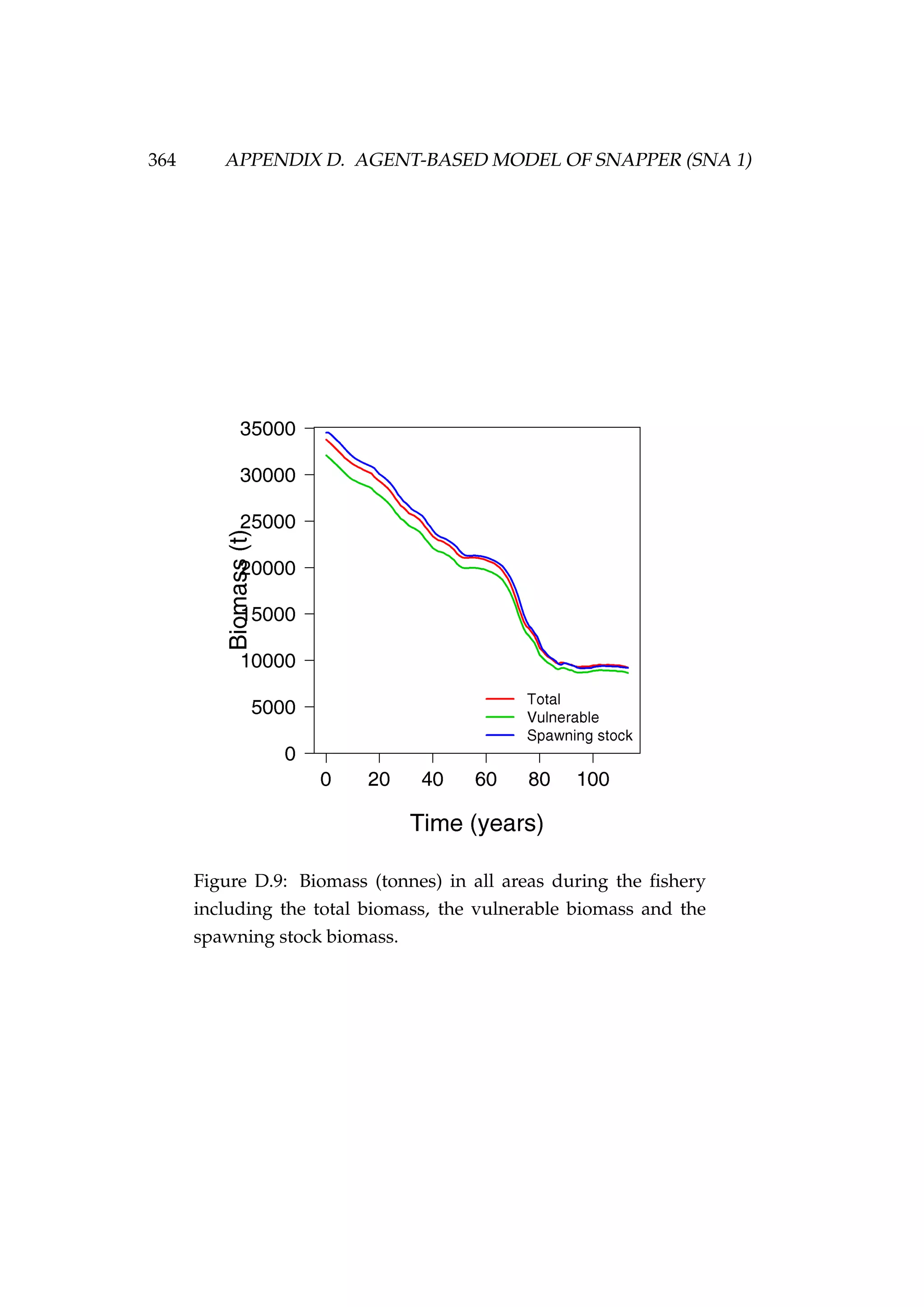
Figure 4.11: Total, vulnerable and spawning stock biomasses
(tonnes) during each year of the fishery [top left] and the total
and vulnerable biomass for each of the three stocks during the
fishery [top right and bottom].

137. 4.7. DISCUSSION 125
model run is done. Preprocessor directive flags within the C++ code indi-
cate how the model is to be structured at compile time including switches
to turn on/off processes such as stochasticity and multithreading. Multi-
threading is done using pthreads. There is some overhead involved when
splitting, passing and collecting multiple threads. A balance must be
struck between the number of threads passed and actual speed gains.
The primary memory (i.e. RAM) required to run the model is a function
of the population size being simulated and the complexity or resolution
desired of the model. Memory problems will arise if trying to simulate
populations with an R0 parameter in the millions of fish with few fish in
each agent (i.e. many agents will be created each year potentially resulting
in billions of agents needing to be stored in the primary memory after
initialisation of the model). The solution is to run the model on a computer
with more RAM, or scale down the size and complexity of the population.
4.7 Discussion
This chapter describes a spatially explicit multi-generational agent-
structured fish simulation model that allows flexibility in specifying pop-
ulation and spatial dynamics. The model has the potential to consider
individual variability, individual movement, and spatial heterogeneity in
the environment. The aim was to construct a model that is sufficiently rich
that it can be used to simulate more complete, realistic fish populations.
The simulated data can be used to test stock assessment methodologies -
which are usually based on samples from the population, and incomplete
data.
In this model, the population is made up of a collection of agents. Agents
are collections of individual fish. The advantage of an agent based model
is that all fish in an agent have identical properties, and can therefore be
treated simultaneously, much like in age-structured models (or the super-
individual concept, Scheffer et al. 1995). However, unlike age-structured
models, an agent can contain a single fish (individual-based), any number
of fish, or an entire cohort of fish (all fish of the same age in the same area

138. 126 CHAPTER 4. AN AGENT-BASED SIMULATION MODEL
in the population). The agents that make up a population can be accessed
and modified to apply standard process including ageing, growth, mat-
uration, recruitment, spawning, natural mortality, fishing mortality and
movement. Special types of migration are also easily implemented, such
as migrations back to the area that the fish recruited to (i.e. home or site
fidelity).
The additional complexity of this model comes at the cost of computa-
tional time and memory. The model can take many hours to do a single
run, and the larger the population that we want to model, the more pri-
mary computer memory (RAM) the model will use. Setting R0 at over
10 million, even with relatively few agents (by specifying that more indi-
viduals may be contained within each agent), results in models that will
use more than 8 GB of RAM. These issues can be solved in one of three
ways: (1) by brute force (using a computer with more RAM and running
for longer); (2) parts of the model could be written the the computers sec-
ondary memory (the hard drive) and the model could be worked on one
part at a time; or (3) by reducing the population size (i.e. using a smaller
R0) or complexity of the model (i.e. fewer areas, allowing agents to merge).
While the structure of this model may be novel in fisheries research, it
may be overly complex as it stretches the limits of even the most mod-
ern high performance computers. As an alternative, one might revert
back to the old matrix-style stock assessment structure while maintain-
ing some of the additional complexity through binning those agent at-
tributes that are measured on a continuous scale and important to the
model (e.g. age-structured models that are also binned by a number of
length-classes or some other variable like home site). For example, per-
sistent individual variation in growth has been approximated by tracking
individual platoons of fishes having the same age but different average
growth rates (Taylor & Methot 2013). Tracking abundance by platoon then
allows stock assessment models to account for the impact of size-selective
fishing on average growth rates.
In describing this model we developed a spatially explicit agent-based
snapper model (for more detail on snapper see Chapter 3, page 77). This

139. 4.7. DISCUSSION 127
snapper model is used later to develop a Bayesian emulator of the agent-
based model in Chapter 7 (page 298). While this model has the capacity to
test many ideas or theories in fished or unfished populations, this was not
the focus of this thesis. However, we discuss the future research potential
for this model below and recommend Thorson et al. (2012) as an example
that does use an ABM to test fisheries theory.
Each agent can store additional information such as agent-specific pa-
rameters relating to size, maturity and natural mortality. Therefore, size-
specific fishing pressure theory may be tested. Many recent studies of
captive or wild populations have demonstrated persistent differences in
behavioural or phenotypic traits among individuals (Shelton et al. 2013,
Webber & Thorson 2015). Persistent differences in activity level or toler-
ance of predation risk (i.e., a tendency to forage in high vs. low-quality
habitat) will likely lead to persistent differences in growth rates among
individuals. Subsequently, persistent differences in growth rate, com-
bined with size-selective harvest targeting larger individuals, can result
in older individuals being composed primarily of slow-growing individ-
uals (termed “Rosa Lees Phenomenon”), and has been demonstrated to
occur in small-lake mesocosm experiments (Biro & Post 2008). In this
way, failure to account for persistent differences in growth rate can lead
to biased estimation of average growth rates in wild populations; popu-
lation dynamics models are increasingly being developed to account for
these effects (Taylor & Methot 2013). Failure to account for such persistent
differences can therefore lead to biases in stock assessment. This model
provides a framework with which to test ideas like these by introducing
different growth models and experimenting with different selectivity pat-
terns.
Agents also have the ability to store information about the agents past,
in essence giving the agent a “memory”. In a spatially-explicit model,
this could allow us to test site fidelity theory and the impacts of hetero-
geneous mixing on estimates of population size. It is well known that
homogeneous mixing is a key assumption of tag-recapture analyses that
aim to estimate population size. Therefore, this model could serve as a
useful platform for testing tag-recapture theory in fish populations and

140. 128 CHAPTER 4. AN AGENT-BASED SIMULATION MODEL
integrated stock assessments.

141. Chapter 5
State-space models
In this chapter we develop biomass dynamics and age-structured state-
space models. We use examples to illustrate the construction and infer-
ence of these models. The biomass dynamics model example uses the
packhorse rock lobster (Sagmariasus verreauxi, PHC) fishery in northern
New Zealand (see Chapter 3, page 80). The age-structured model example
uses the snapper (Pagurus auratus, SNA) fishery in northern New Zealand
(SNA 1, see Chapter 3, page 77).
5.1 Introduction
Commercial and ecological management of fisheries requires good esti-
mates of stock sizes. These estimates are obtained by modelling fish pop-
ulation dynamics. The models are fitted to commercial fisheries data,
and/or information collected independently of the commercial fishery.
Generally these data are patchy in space and time and not collected ran-
domly, breaking almost all of the assumptions of classical statistical mod-
els and tests. These models should provide estimates with as little bias
as possible and the uncertainty in the data should be properly reflected
in the estimates produced by the models. Therefore, stock assessment
models should have the ability to deal with uncertainty and adequately
convey the uncertainty in the estimates they provide. Current stock as-
129

142. 130 CHAPTER 5. STATE-SPACE MODELS
sessment models tend to underestimate the true uncertainty (Magnusson
et al. 2013). This can produce biased results (Mormede, Dunn & Hanchet
2013) which can lead to incorrect inferences (Hoshino et al. 2014).
State-space models incorporate both observation and process uncertainty.
State-space models are statistical Markov models, also known as hidden
Markov models (HMM) or latent state models, in which the system is as-
sumed to be a Markov process with unobserved (hidden) states. Specifi-
cally, state-space models relate observations yt (e.g. CPUE) at a time t to
unobserved states xt (e.g. biomass) through stochastic observation equa-
tions for yt. Stochastic transition equations define how the hidden states
(xt) are assumed to evolve in time. An observed or specified control vari-
able or covariate (zt) may also be included in a state-space system (e.g.
catch). Thus, the process model could take the form xt = f(xt−1, zt, θ) + εp
t
and the observation model yt = g(xt, zt, θ) + εo
t where θ are model param-
eters, εo
t are observation errors, and εp
t are process errors. These equations
can be represented graphically as:
· · · xt−1 xt xt+1 · · ·
yt−1 yt yt+1
zt−1 zt zt+1
By incorporating both observation and process error, state-space models
can help us better quantify the uncertainty of parameters of interest (Har-
wood & Stokes 2003). State-space models can incorporate variability in
key population parameters by allowing these parameters to follow a first
order autoregressive process over time. Also, state-space features in mod-
els can help reduce the number of model parameters (Nielsen & Berg
2014).
For example, state-space methods have been used to some extent in age-
structured models to estimate time-varying selectivity and random walk
fishing mortalities (Butterworth et al. 2003, Nielsen & Berg 2014). Al-
though state-space models have had some limited use in fisheries mod-
elling they are the exception rather than the norm, particularly in age-
structured models. However, Meyer & Millar (1999) have developed basic

143. 5.1. INTRODUCTION 131
state-space biomass dynamics models.
Fully state-space age-structured models that estimate the numbers of fish
at age each year (Na,t) as a latent state are almost absent from the liter-
ature. However, Millar & Meyer (2000) develop an age-structured model
that treats total mortality (Ma,t being made up of natural mortality and un-
reported catch) as being state-space. We describe this model briefly below,
but for more detail see their original paper. Their process model is
Na,t = Na−1,t−1e−Ma,t
− Ca,te−0.5Ma,t
,
where Na,t is the mid-year numbers at age a and time t, Ca,t is the catch
in numbers at age and time, and in their Bayesian framework they specify
the priors
Ma,t ∼ log N µa, τ2
,
µa ∼ N ν, σ2
,
τ2
∼ IG (α, β) .
In this way, setting ν = log(0.2) gives each Ma,t a prior median of 0.2 and
a high value of σ2
represents little prior confidence that each Ma,t is close
to 0.2 and independent of age. Similarly, a high variance hyper-prior for
τ2
suggests that we have little prior belief in Ma,t being constant over time
within each age-class. Their model was developed for an example where
• data are indices of numbers-at-age from research vessel surveys
(Ia,t = log N (log (qaNa,t) , σ2
))
• reported catch is provided as numbers-at-age (Ca,t)
This is a little bit of an unrealistic data set by New Zealand standards as
age-structured catch and therefore CPUE data are very hard to come by.
They also admit that, for a variety of reasons, “it would be inappropriate
to use the results from their model for inference about current stock status
or for risk management”.
Despite considerable interest in state-space models, and previous work
suggesting that they have superior performance when compared with de-
terministic models (Millar & Meyer 2000), they are not widely used, likely

144. 132 CHAPTER 5. STATE-SPACE MODELS
due to their added complexity in implementation. Quinn (1992) raises the
point that “few statisticians have been involved in fisheries modelling and
that this has resulted in a whole class of methods unlike anything found
in the mainstream statistics literature”. Whether or not this is a good thing
is up for discussion.
Much of the existing work on state-space modelling in fisheries has used
maximum likelihood inference methods. However, it can be difficult to
estimate both observation and process error simultaneously using maxi-
mum likelihood methods (Meyer & Millar 1999). Therefore, sticking to the
theme of this thesis, we limit our inference to Bayesian methods only.
Before we get into fisheries state-space models, we present a very simple
(non state-space) example to illustrate some concepts in basic inference.
We then introduce state-space fisheries models with a brief example using
biomass dynamics models. These models were first introduced in Chap-
ter 1, page 35. Biomass dynamics models are the the method of choice
(and really the only method available) if the only data available include a
times series of catches and an index of abundance (Punt 2003a). Finally, we
reformulate age-structured models, first introduced in Chapter 1, page 37,
to include process error associated with the numbers of fish at age and
time (Na,t) within the population. The major contribution provided in this
chapter is the construction of the posterior for a state-space age-structured
model. While this model has the potential to better represent uncertainty
in stock assessment, we warn that its practical application remains limited
as MCMC mixing was unsatisfactory. The future challenge is to sample
from this posterior efficiently.
5.2 A simple example
We begin with a very simple (non state-space) model that we use to il-
lustrate the accuracy that can be expected when simulating from a model,
then back estimating parameters used in the simulation model. The model

145. 5.2. A SIMPLE EXAMPLE 133
has parameters a and σ2
ε and covariates zt for time steps t = 1, . . . , T
yt = azteεt−σ2
ε /2
where εt
iid
∼ N 0, σ2
ε , (5.1)
where −σ2
ε /2 is a log-normal correction term (see Appendix A.2 for proof).
The observations (yt) are therefore assumed to be log-normal random vari-
ables
log (yt) |zt, a, σ2
ε ∼ N log (azt) − σ2
ε /2, σ2
ε . (5.2)
We simulate from this model for T = 100 time steps, setting a = 3 and
σε = 0.1.
We are interested in the probabilistic relationship between the following:
• The data: y = {yt}T
t=1
• The covariates: z = {zt}T
t=1
• The parameters of interest: θ = {a, σ2
ε }
Using Bayes theorem, the posterior distribution of the model parameters
(θ), given the data (y) and covariates (z) is
π (θ|y, z) ∝ π (θ) π (y|z, θ) , (5.3)
where the prior and the likelihood are
π (θ) = π a, σ2
ε = π(a)π σ2
ε ,
π (y|z, θ) = π y|z, a, σ2
ε =
T
t=1
π yt|zt, a, σ2
ε .
Using MCMC we can sample from the posterior distribution (Equa-
tion 5.3) to obtain probability distributions of the model parameters. We
placed uniform priors with wide bounds on both parameters specifying
a ∼ U(−9e99, 9e99) and σε ∼ U(0, 9e99). We ran our MCMC for 100,000
iterations, with a thinning rate of 10 resulting a sample size of 10,000. The
MCMC burn-in was 1000 iterations and the standard deviation of the log-
normal proposal distribution was set to σq = 0.05 (see Chapter 2, page 66
for a description of MCMC using a log-normal proposal distribution). We
repeat using different random number seeds in three different simulated

146. 134 CHAPTER 5. STATE-SPACE MODELS
Figure 5.1: MCMC trace plots [left] and posterior densities
[right] for the model parameters (a and σε) and the log-
likelihood of the model. The true values of the model parame-
ters in the simulation are indicated as solid blue lines in the top
two panels. The log-prior was not plotted as it was constant in
this example.

147. 5.2. A SIMPLE EXAMPLE 135
Figure 5.2: MCMC trace plots [left] and posterior densities
[right] for the model parameters (a and σε) and the log-
likelihood of the model. The true values of the model parame-
ters in the simulation are indicated as solid blue lines in the top
two panels. The log-prior was not plotted as it was constant in
this example.

148. 136 CHAPTER 5. STATE-SPACE MODELS
Figure 5.3: MCMC trace plots [left] and posterior densities
[right] for the model parameters (a and σε) and the log-
likelihood of the model. The true values of the model parame-
ters in the simulation are indicated as solid blue lines in the top
two panels. The log-prior was not plotted as it was constant in
this example.

149. 5.3. BIOMASS DYNAMICS STATE-SPACE MODELS 137
data sets. MCMC trace plots and densities are shown in Figures 5.1, 5.2
and 5.3. These results show a model that is working well. All chains have
converged and the true values are within credible intervals.
5.3 Biomass dynamics state-space models
A biomass dynamics state-space model relates catch per unit effort ob-
servations (It) to the unobserved biomass states (Bt) through a stochastic
observation model for It given by
It = qBteεo
t −σ2
o/2
where εo
t
iid
∼ N 0, σ2
o , (5.4)
where q is the catchability coefficient and εo
t is the normally distributed
observation error at time t with variance σ2
o. The states are assumed to
follow a stochastic transition model of surplus production
Bt = Bt−1 + rBt−1 1 −
Bt−1
K
− Ct−1 eεp
t −σ2
p/2
where εp
t
iid
∼ N 0, σ2
p ,
(5.5)
where Ct is the catch (tonnes) at time t, r is the intrinsic rate of popula-
tion increase, K is the carrying capacity (tonnes), and εp
t is the normally
distributed process error at time t with variance σ2
p.
Due to known difficulties with the parameterisation in Equation 5.5 lead-
ing to poor performance in the Metropolis-Hastings sampler it is com-
mon practice to reparameterise the model by replacing the states Bt with
Jt = Bt/K (Meyer & Millar 1999). The new states are the ratio of biomass
to carrying capacity also known as depletion. Thus Bt is replaced by KJt,
and the form becomes
log(Jt) ∼ N log (µ1) − σ2
p/2, λ1σ2
p t = 1,
Jt = Jt−1 + rJt−1(1 − Jt−1) −
Ct−1
K
eεp
t −σ2
p/2
t = 2, . . . , T,
It = qKJteεo
t −σ2
o/2
∀t. (5.6)
The states (Jt) and observations (It) are therefore assumed to be log-

150. 138 CHAPTER 5. STATE-SPACE MODELS
normal random variables
log(J1)|µ1, λ1, σ2
p ∼ N log (µ1) − σ2
p/2, λ1σ2
p ,
log(Jt)|Jt−1, r, K, σ2
p, Ct−1 ∼ N log Jt−1 + rJt−1(1 − Jt−1) −
Ct−1
K
− σ2
p/2, σ2
p ,
log(It)|K, q, σ2
o, Jt ∼ N log (qKJt) − σ2
o/2, σ2
o . (5.7)
Usually it is assumed that µ1 = 0 and λ1 = 1 (i.e. the biomass in the first
year is at carrying capacity B1 = K) and we make this assumption here.
This model can be represented graphically as:
B1 = K B2 · · · Bt · · · BT BT+1
I1 I2 It IT
C1 Ct−1 CT−1 CT
In summary, this model makes the following assumptions:
• the parameters r, K, and q are constant over time t
• the intrinsic rate of population increase (r) is independent of the
age/size composition of the population
• the population is at its carrying capacity (K) at the start of the model
(i.e. B1 = K)
• the population is closed (no immigration or emigration)
• fishing and natural mortality are applied simultaneously
• the catch (Ct) is measured without error
• the CPUE (It) is proportional to abundance (Bt).
5.3.1 Inference
We are interested in the probabilistic relationship between the following:
• The data y: the catch per unit effort (It). Let y = {It}T
t=1

151. 5.3. BIOMASS DYNAMICS STATE-SPACE MODELS 139
• The covariates z: the catch (Ct). Let z = {Ct}T
t=1
• The unknown parameters of interest θ: the intrinsic rate of popula-
tion increase (r) and the carrying capacity of the population (K). Let
θ = {r, K}
• The unknown nuisance parameters ω: the catchability coefficient
(q) and the observation and process error variances (σ2
o and σ2
p). Let
ω = {q, σ2
o, σ2
p}
• The unknown latent states x: the depletion (Jt). Let x = {Jt}T
t=1
Using Bayes theorem, the posterior distribution of the model parameters
(θ and ω) and the states (x), given the data (y) and covariates (z) is
π(θ, ω, x|y, z) ∝ π(θ, ω, x|z)π(y|θ, ω, x), (5.8)
where
π (θ, ω, x|z) = π r, K, q, σ2
o, σ2
p, x|z
= π(r)π(K)π(q)π(σ2
o)π(σ2
p)π x|z, r, K, σ2
p
= π(r)π(K)π(q)π(σ2
o)π(σ2
p)π J1|K, σ2
p
T
t=2
π Jt|Jt−1, Ct−1, r, K, σ2
p ,
π (y|x, θ, ω) = π y|x, K, q, σ2
o =
T
t=1
π It|Jt, K, q, σ2
o . (5.9)
Using MCMC we can sample from the posterior distribution (Equa-
tion 5.8) to obtain probability distributions of the parameters, latent states
and other quantities of interest in the model (e.g. the biomass Bt). We
provide an example below (Section 5.3.2).
Using Equations 5.7 and 5.8 and the priors described below we esti-
mate posterior distributions for each of the parameters using blockwise
Metropolis-Hastings using log-normal proposals (see Chapter 2, page 66).
It is well known that the parameters r and K are highly correlated. To re-
duce this correlation and improve MCMC performance we set φ1 = rK
and φ2 = r/K and propose φ1 and φ2 in the MCMC instead (Gilks &
Roberts 1996). One can solve for r and K when required
r = φ1φ2 and K =
φ1
φ2
.

152. 140 CHAPTER 5. STATE-SPACE MODELS
If a transformation like this is used then the priors for these two parame-
ters must be updated using the Jacobian
K r
1
K
− r
K2
=
∂(φ1, φ2)
∂(r, K)
= −
r
K
−
r
K
= −
2r
K
= 2φ2,
thus the prior for the two parameters becomes
π(φ1, φ2) = π(r)π(K)
∂(r, K)
∂(φ1, φ2)
= π(r)π(K)
1
2φ2
= π(r)π(K)
K
2r
.
See Chapter 2, page 67, for notes on parameter transformations in MCMC.
Therefore, the acceptance probability is
r = min 1,
π(y|θ∗
)
π(y|θ(i−1)
)
×
π(θ∗
)
π(θ(i−1)
)
×
qθ(θ(i−1)
|θ∗
, y)
qθ(θ∗
|θ(i−1)
, y)
= min 1,
π(y|θ∗
)
π(y|θ(i−1)
)
×
π(θ∗
)
π(θ(i−1)
)
×
θ∗
θ(i−1)
= min 1,
π(y|θ∗
)
π(y|θ(i−1)
)
×
π(r∗
)
π(r(i−1))
×
π(K∗
)
π(K(i−1))
×
π(q∗
)
π(q(i−1))
×
π(σ2∗
o )
π(σ
2(i−1)
o )
×
π(σ2∗
p )
π(σ
2(i−1)
p )
×
K∗
2r∗
K(i−1)
2r(i−1)
×
θ∗
θ(i−1)
.
5.3.2 Packhorse rock lobster example
Simulation
We simulate data based on the packhorse rock lobster (Sagmariasus ver-
reauxi, PHC) fishery in northern New Zealand using Equations 5.4 and 5.5
(for more information on the fishery see Chapter 3, page 80). We use a
set of plausible parameter values in each simulation (Table 5.1). There is
always considerable uncertainty in estimates of the observation and pro-
cess error within these models (McAllister et al. 2001), so two different
simulations were done setting the observation and process error standard
deviations (σo and σp) to low and high values. The high values might
sit somewhere close to what is realistic. It is important that there is con-
trast (i.e. a clear trend over time) in the CPUE time series to get a good fit

153. 5.3. BIOMASS DYNAMICS STATE-SPACE MODELS 141
Table 5.1: Parameter values used in packhorse rock lobster simulation.
Parameter Value Units Description
r 0.17 - Intrinsic rate of population
increase
K 1800 tonnes Carrying capacity
q 0.002 tonnes−1 Catchability coefficient
σo 0.01, 0.1 - Observation error standard
deviation
σp 0.001, 0.01 tonnes Process error standard devi-
ation
using a biomass dynamics models (this is also true of age-structured mod-
els, Hilborn & Walters 1992). The actual catch history of the packhorse rock
lobster fishery is used in both simulation runs and provides adequate con-
trast in the simulated CPUE when using the parameters specified above
(Figure 5.4). The simulated CPUE (It) and biomass (Bt) are given for vari-
Figure 5.4: True catch history (Ct, tonnes) of the packhorse rock
lobster from 1953 to 2012 (60 years) used in the simulation.
ous scenarios in Figures 5.6, 5.8, 5.10, 5.12, 5.14 and 5.16 below. We discuss
each of these scenarios in turn.

154. 142 CHAPTER 5. STATE-SPACE MODELS
Estimation with highly informative priors
We begin by specifying highly informative priors for each of the model pa-
rameters to check for any problems in the model or MCMC specification.
The full list of priors is
π(r) ∼ log N(log(0.17), 0.01),
π(K) ∼ log N(log(1800), 0.005),
π(q) ∼ log N(log(0.002), 0.005),
π(σ2
o) ∼ log N(log(0.012
), 0.05) or π(σ2
o) ∼ log N(log(0.12
), 0.05),
π(σp) ∼ log N(log(0.001), 0.1) or π(σp) ∼ log N(log(0.01), 0.1), (5.10)
noting that priors are applied to the variance of observation error (σ2
o) and
to the standard deviation of process error (σp).
We ran three million iterations using blockwise Metropolis-Hastings with
log-normal proposals (see Chapter 2, page 66). These three million itera-
tions were run as three separate MCMC chains on three different computer
cores, all initialised with different random number seeds. Each chain ran
an additional burn-in of two million iterations. The chains were thinned
to save every 1000th iteration. This resulted in a total of 3000 samples of
the posterior distribution for each of the parameters and latent states.
In the low observation and process error model (σo = 0.01, σp = 0.001),
all parameters were recovered well with the mode of the posterior distri-
bution for each parameter centered near the true value (Figure 5.5). The
densities of the observation error variance (σ2
o) and standard deviation of
process error (σp) are not constrained by the data and MCMC is simply
recovering the prior. The mode of the catchability coefficient (q) is the pa-
rameter furtherest from the true value set in the simulation. Despite this,
the model fits the CPUE (It) observations well and results in a good match
between the posterior biomass trajectory (Bt) and the simulated biomass
trajectory (Figure 5.6).
In the high observation and process error model (σo = 0.1, σp = 0.01), the
parameters were also well estimated (Figure 5.7). Again, the densities of
the observation error variance (σ2
o) and standard deviation of process error

155. 5.3. BIOMASS DYNAMICS STATE-SPACE MODELS 143
Figure 5.5: MCMC trace plots and posterior densities for the
model parameters using data from the low observation error
(σo = 0.01) and process error (σp = 0.001) model estimated
using highly informative priors. Posterior traces and densities
are indicated as black lines, priors as dashed black lines, and
values specified in simulation as solid blue lines.

156. 144 CHAPTER 5. STATE-SPACE MODELS
Figure 5.6: Fit to CPUE observations (It) [left] and the poste-
rior distribution of biomass (Bt) [right] for the low observation
error (σp = 0.01) and process error (σp = 0.001) model esti-
mated using highly informative priors. CPUE observations
are shown as black points [•] and the posterior distribution of
the fit to CPUE is shown in blue. The posterior distribution of
biomass is shown in green and the simulated biomass as the
dashed black line. The shading indicates the 5th, 25th, 50th,
75th and 95th percentiles.

157. 5.3. BIOMASS DYNAMICS STATE-SPACE MODELS 145
Figure 5.7: MCMC trace plots and posterior densities for the
model parameters using data from the high observation error
(σo = 0.1) and process error (σp = 0.01) model estimated us-
ing highly informative priors. Posterior traces and densities
are indicated as black lines, priors as dashed black lines, and
values specified in simulation as solid blue lines.

158. 146 CHAPTER 5. STATE-SPACE MODELS
(σp) are not constrained by the data and MCMC is simply recovering the
prior. The model fits the CPUE (It) observations well and the estimated
biomass trajectory (Bt) is biased high only a little when compared with
the simulated biomass trajectory (Figure 5.8).
Figure 5.8: Fit to CPUE observations (It) [left] and the posterior
distribution of biomass (Bt) [right] for the high observation er-
ror (σp = 0.1) and process error (σp = 0.01) model estimated us-
ing highly informative priors. CPUE observations are shown
as black points [•] and the posterior distribution of the fit to
CPUE is shown in blue. The posterior distribution of biomass
is shown in green and the simulated biomass as the dashed
black line. The shading indicates the 5th, 25th, 50th, 75th and
95th percentiles.
Relaxing the priors on r, K and q
We relax the priors placed on r, K and q and repeat. Usually we have no
prior knowledge of the value of K and q. It it standard practice in fisheries
to use uniform priors with wide bounds for almost all model parameters
so that the priors are as uninformative as possible (in the absence of any
prior information of course). Instead of using improper uniform priors in

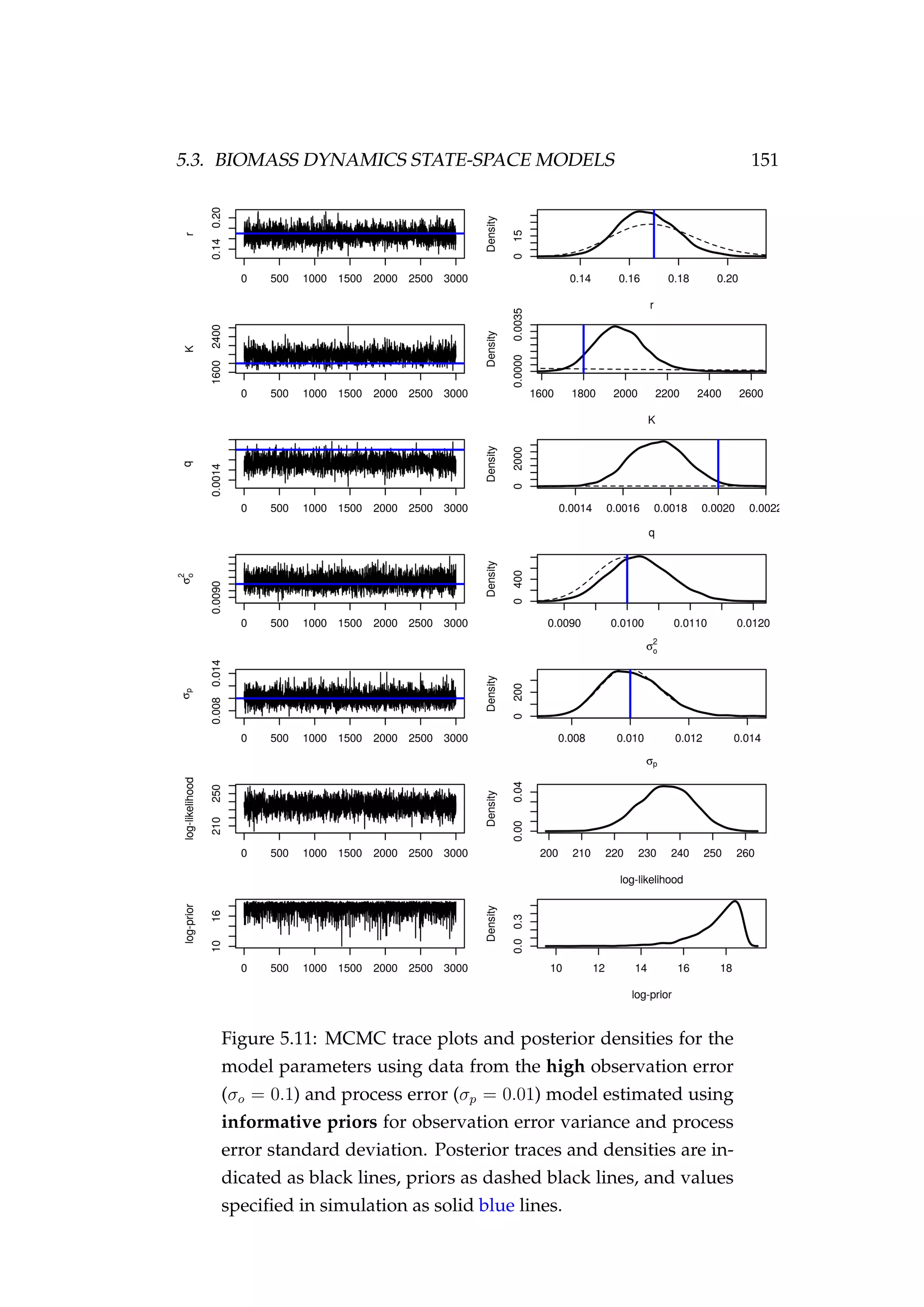
159. 5.3. BIOMASS DYNAMICS STATE-SPACE MODELS 147
this way, which can lead to poor MCMC mixing and may result in a lack of
convergence, we use a range of uninformative continuous proper priors.
For the parameters K and q we develop uninformative log-normal priors.
Instead of using a uniform with wide bounds a and b
X ∼ U(a, b),
we assume that there is some negligibly small probability that parameter
X will be below a or above b (e.g. 1%) and use a log-normal prior
log(X) ∼ N µ, σ2
where E[log(X)] = µ and V[log(X)] = σ.
We can write
P(X < a) = P (log(X) < log(a)) = P zα <
log(a) − µ
σ
= α,
P(X < b) = P (log(X) < log(b)) = P zβ <
log(b) − µ
σ
= β,
or
zα =
log(a) − µ
σ
and zβ =
log(b) − µ
σ
.
Solving for µ and σ we get
µ =
zα log(b) − zβ log(a)
zα − zβ
and σ =
log(b) − log(a)
zβ − zα
. (5.11)
For example, setting α = 1% and β = 99% would yield zα = −2.326 and
zβ = 2.326.
For the parameter K we set a = 100 and b = 10000, with α = 1% and
β = 99%. For q we set a = 0.001 and b = 1, with α = 1% and β =
99%. The priors derived from these are provided below (Equation 5.12).
Finally, some work has gone into the development of informed priors for
use in biomass dynamics models (McAllister et al. 2001), particularly for
the parameter r. Therefore, we assume some prior knowledge of r. The
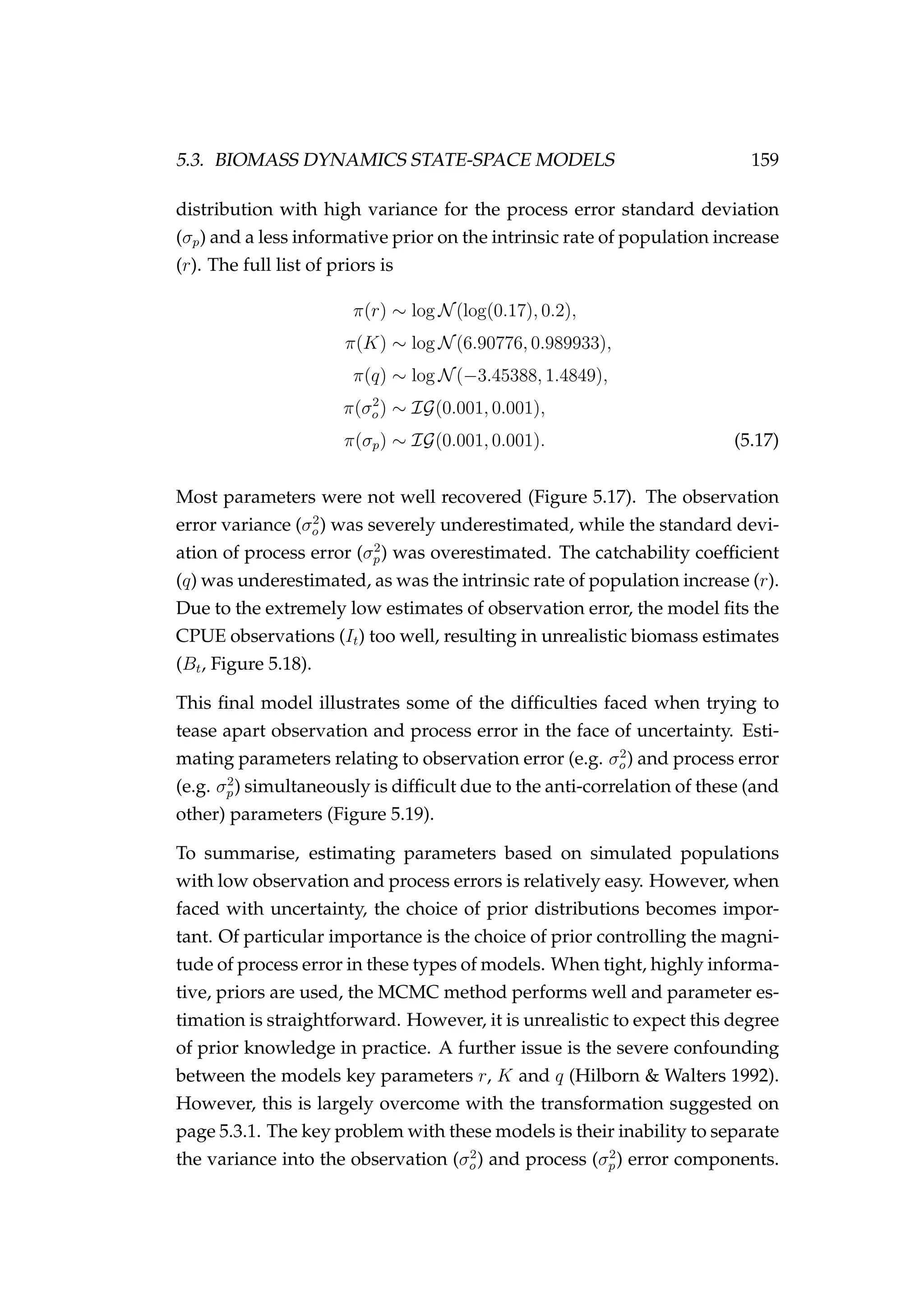
full list of priors is
π(r) ∼ log N(log(0.17), 0.1),
π(K) ∼ log N(6.90776, 0.989933),
π(q) ∼ log N(−3.45388, 1.4849),
π(σ2
o) ∼ log N(log(0.012
), 0.05) or π(σ2
o) ∼ log N(log(0.12
), 0.05),
π(σp) ∼ log N(log(0.001), 0.1) or π(σp) ∼ log N(log(0.01), 0.1), (5.12)

160. 148 CHAPTER 5. STATE-SPACE MODELS
In the low observation and process error model (σo = 0.01, σp = 0.001),
parameters were not recovered as well as before (Figure 5.9). The densi-
ties of the observation error variance (σ2
o) and standard deviation of pro-
cess error (σp) are not constrained by the data and the MCMC is simply
recovering the prior. The mode of the catchability coefficient (q) and the
carrying capacity (K) were quite far from the true value set in the simu-
lation. Despite this, the model fits the CPUE (It) observations well and
results in a good match between the posterior biomass trajectory (Bt) and
the simulated biomass trajectory (Figure 5.10).
In the high observation and process error model (σo = 0.1, σp = 0.01), most
parameters were not well recovered (Figure 5.11). Again, the densities of
the observation error variance (σ2
o) and standard deviation of process error
(σp) are not constrained by the data and MCMC is simply recovering the
prior. The catchability coefficient (q) was underestimated and the carrying
capacity (K) overestimated. While the model fit to the CPUE observations
(It) looks adequate, the biomass (Bt) is consistently overestimated (Fig-
ure 5.12).
Relaxing the priors on π(σ2
o) and π(σp)
The inverse gamma distribution with high variance is recommended as
a good choice of uninformative prior for variance parameters (Gelman
2006). However, we found that MCMC generally resulted in us underesti-
mating the observation error variance (σ2
o) and over estimating the process
error standard deviation (σp). Therefore, we develop a prior for σp. In do-
ing so we consider how much it might be reasonable for the population
biomass to be changing from year to year. We do this assuming a closed
population (i.e. the effects of migration and other things that could af-
fect the biomass are negligible). Let’s say that in most circumstances we
would not expect the population biomass to be different by more than 10%
between any two years, after taking into account production and the catch.
This would yield
0.9 ≤ eεp
t ≤ 1.1 or log(0.9) ≤ εp
t ≤ log(1.1).

161. 5.3. BIOMASS DYNAMICS STATE-SPACE MODELS 149
Figure 5.9: MCMC trace plots and posterior densities for the
model parameters using data from the low observation error
(σo = 0.01) and process error (σp = 0.001) model estimated us-
ing informative priors for observation error variance and pro-
cess error standard deviation. Posterior traces and densities are
indicated as black lines, priors as dashed black lines, and val-
ues specified in simulation as solid blue lines.

162. 150 CHAPTER 5. STATE-SPACE MODELS
Figure 5.10: Fit to CPUE observations (It) [left] and the pos-
terior distribution of biomass (Bt) [right] for the low observa-
tion error (σp = 0.01) and process error (σp = 0.001) model
estimated using informative priors for observation error vari-
ance and process error standard deviation. CPUE observations
are shown as black points [•] and the posterior distribution of
the fit to CPUE is shown in blue. The posterior distribution of
biomass is shown in green and the simulated biomass as the
dashed black line. The shading indicates the 5th, 25th, 50th,
75th and 95th percentiles.

163. 5.3. BIOMASS DYNAMICS STATE-SPACE MODELS 151
Figure 5.11: MCMC trace plots and posterior densities for the
model parameters using data from the high observation error
(σo = 0.1) and process error (σp = 0.01) model estimated using
informative priors for observation error variance and process
error standard deviation. Posterior traces and densities are in-
dicated as black lines, priors as dashed black lines, and values
specified in simulation as solid blue lines.

164. 152 CHAPTER 5. STATE-SPACE MODELS
Figure 5.12: Fit to CPUE observations (It) [left] and the pos-
terior distribution of biomass (Bt) [right] for the high obser-
vation error (σp = 0.1) and process error (σp = 0.01) model
estimated using informative priors for observation error vari-
ance and process error standard deviation. CPUE observations
are shown as black points [•] and the posterior distribution of
the fit to CPUE is shown in blue. The posterior distribution of
biomass is shown in green and the simulated biomass as the
dashed black line. The shading indicates the 5th, 25th, 50th,
75th and 95th percentiles.

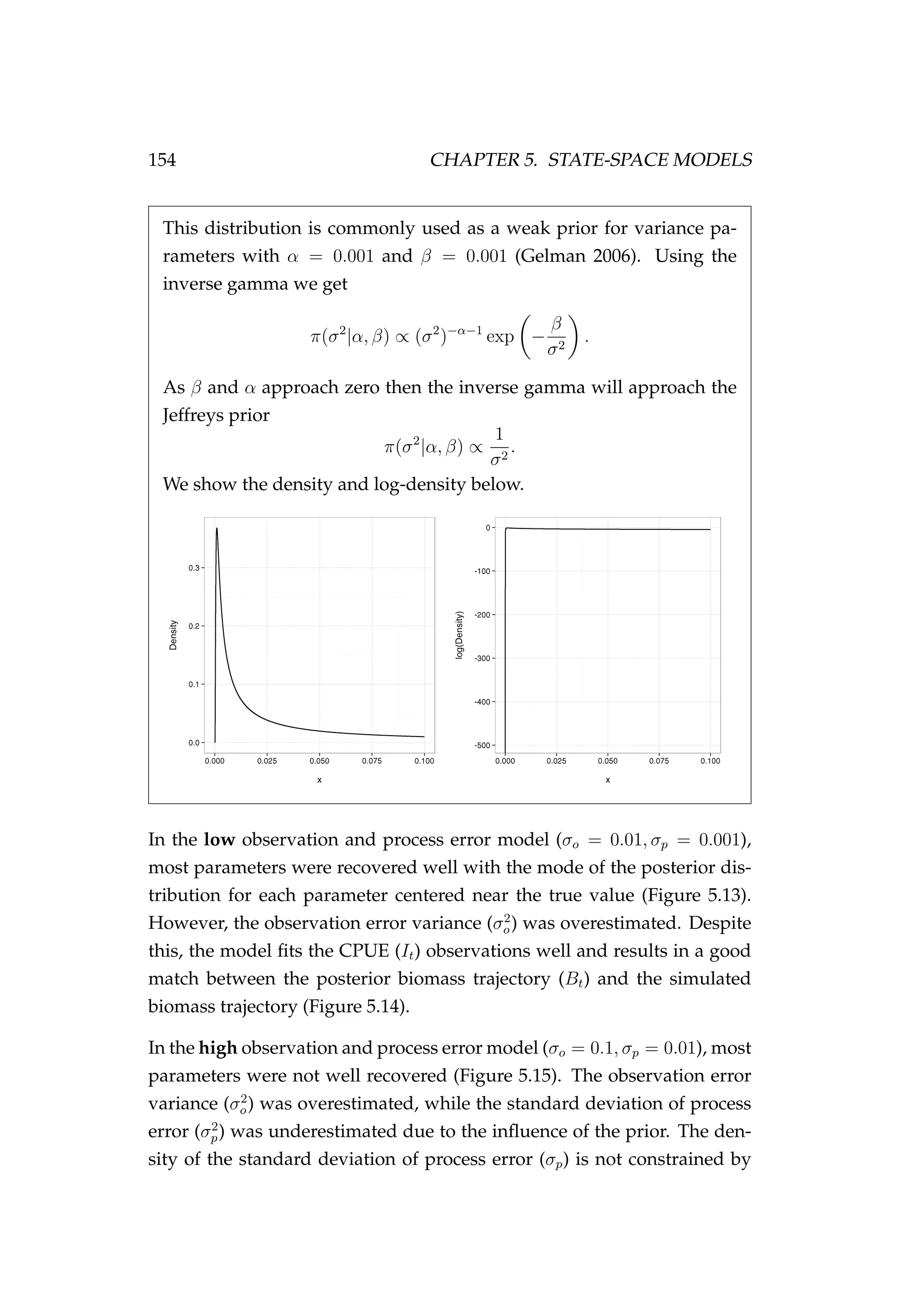
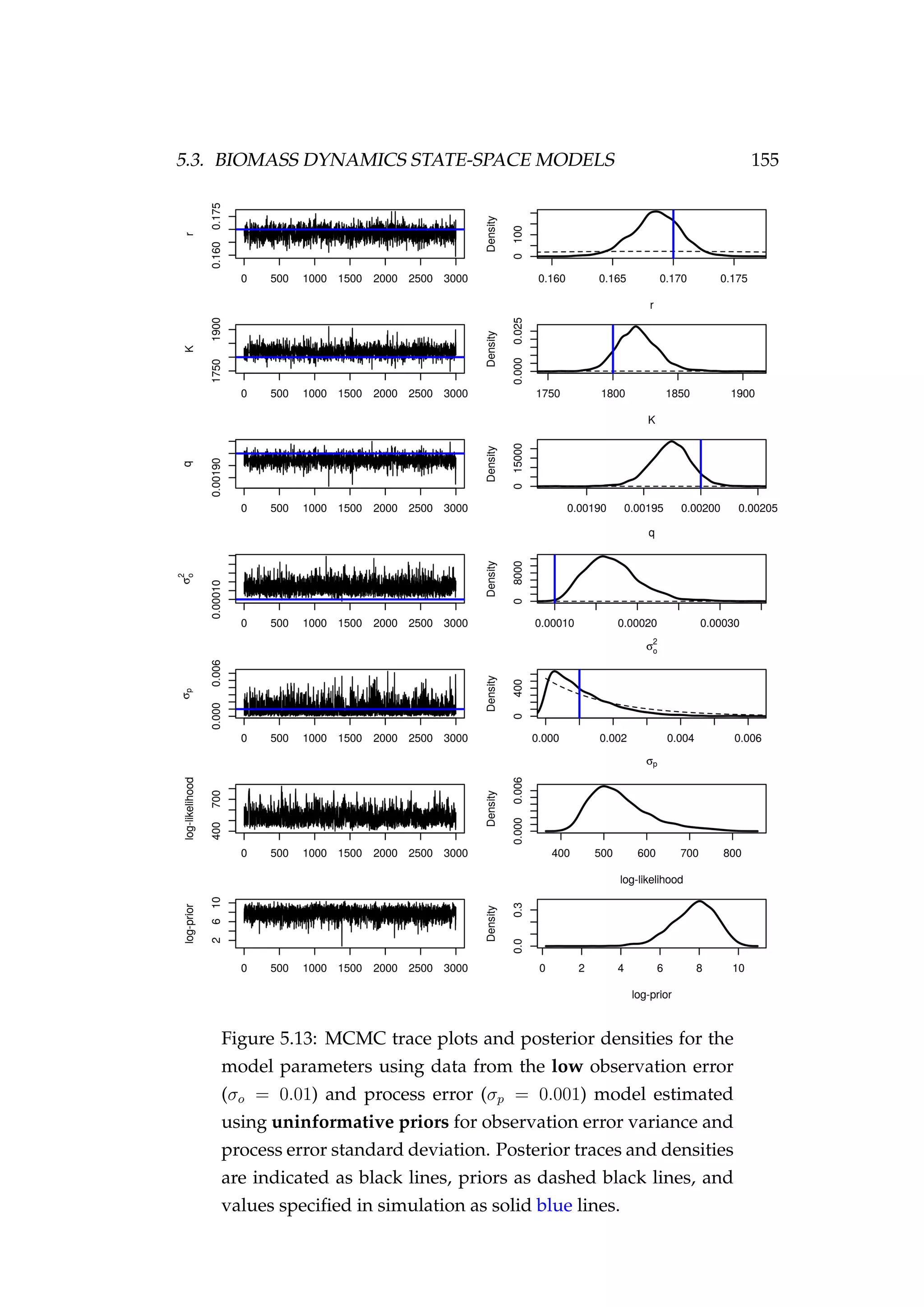
165. 5.3. BIOMASS DYNAMICS STATE-SPACE MODELS 153
We can generalise this and write
log(a) ≤ eεp
t ≤ log(b). (5.13)
We then solve for the process error standard deviation (σp)
σp =
log(b) − log(a)
zβ − zα
≈ 0.043. (5.14)
Thus, we state that σp should be less than or equal to the value derived
above. To capture this property we place a gamma prior distribution on
σp with α = 1 (i.e. an exponential). Thus
π(σp) ∼ Ga(α, β),
E[σp] =
α
β
=
1
β
= 0.043,
∴ β ≈ 23, (5.15)
The full list of priors is
π(r) ∼ log N(log(0.17), 0.1),
π(K) ∼ log N(6.90776, 0.989933),
π(q) ∼ log N(−3.45388, 1.4849),
π(σ2
o) ∼ IG(0.001, 0.001),
π(σp) ∼ Ga(1, 23). (5.16)
The inverse gamma distributions density function is defined over the
support x > 0 with shape parameter α and scale parameter β
f(x|α, β) =
βα
Γ(α)
x−α−1
exp −
β
x
,
where
E(x) =
β
α + 1
for α > 1,
V(x) =
β2
(α − 1)2α − 2()
for α > 2.

166. 154 CHAPTER 5. STATE-SPACE MODELS
This distribution is commonly used as a weak prior for variance pa-
rameters with α = 0.001 and β = 0.001 (Gelman 2006). Using the
inverse gamma we get
π(σ2
|α, β) ∝ (σ2
)−α−1
exp −
β
σ2
.
As β and α approach zero then the inverse gamma will approach the
Jeffreys prior
π(σ2
|α, β) ∝
1
σ2
.
We show the density and log-density below.
In the low observation and process error model (σo = 0.01, σp = 0.001),
most parameters were recovered well with the mode of the posterior dis-
tribution for each parameter centered near the true value (Figure 5.13).
However, the observation error variance (σ2
o) was overestimated. Despite
this, the model fits the CPUE (It) observations well and results in a good
match between the posterior biomass trajectory (Bt) and the simulated
biomass trajectory (Figure 5.14).
In the high observation and process error model (σo = 0.1, σp = 0.01), most
parameters were not well recovered (Figure 5.15). The observation error
variance (σ2
o) was overestimated, while the standard deviation of process
error (σ2
p) was underestimated due to the influence of the prior. The den-
sity of the standard deviation of process error (σp) is not constrained by

167. 5.3. BIOMASS DYNAMICS STATE-SPACE MODELS 155
Figure 5.13: MCMC trace plots and posterior densities for the
model parameters using data from the low observation error
(σo = 0.01) and process error (σp = 0.001) model estimated
using uninformative priors for observation error variance and
process error standard deviation. Posterior traces and densities
are indicated as black lines, priors as dashed black lines, and
values specified in simulation as solid blue lines.

168. 156 CHAPTER 5. STATE-SPACE MODELS
Figure 5.14: Fit to CPUE observations (It) [left] and the poste-
rior distribution of biomass (Bt) [right] for the low observation
error (σp = 0.01) and process error (σp = 0.001) model esti-
mated using uninformative priors for observation error vari-
ance and process error standard deviation. CPUE observations
are shown as black points [•] and the posterior distribution of
the fit to CPUE is shown in blue. The posterior distribution of
biomass is shown in green and the simulated biomass as the
dashed black line. The shading indicates the 5th, 25th, 50th,
75th and 95th percentiles.

169. 5.3. BIOMASS DYNAMICS STATE-SPACE MODELS 157
Figure 5.15: MCMC trace plots and posterior densities for the
model parameters using data from the high observation error
(σo = 0.01) and process error (σp = 0.001) model estimated
using uninformative priors for observation error variance and
process error standard deviation. Posterior traces and densities
are indicated as black lines, priors as dashed black lines, and
values specified in simulation as solid blue lines.

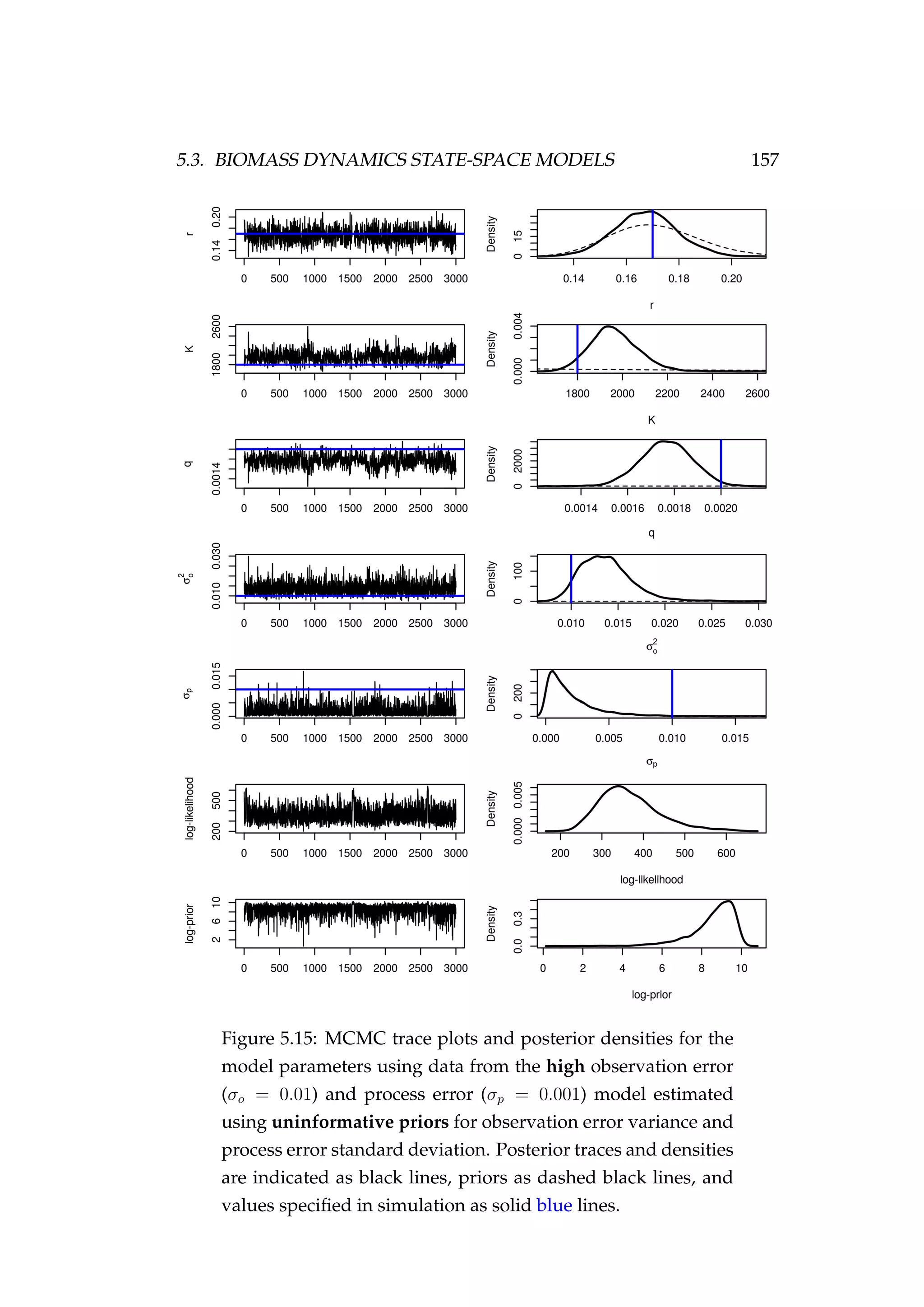
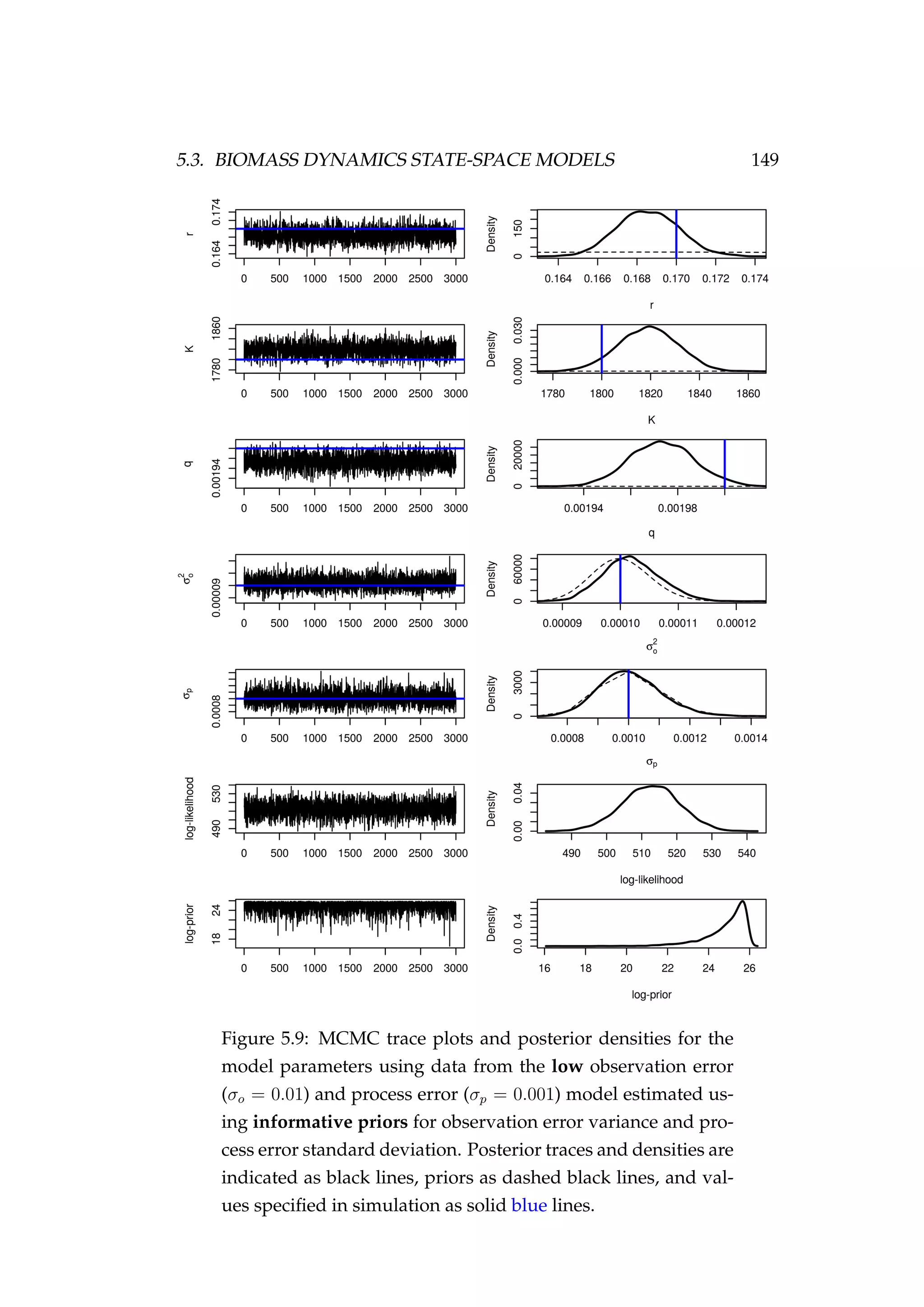
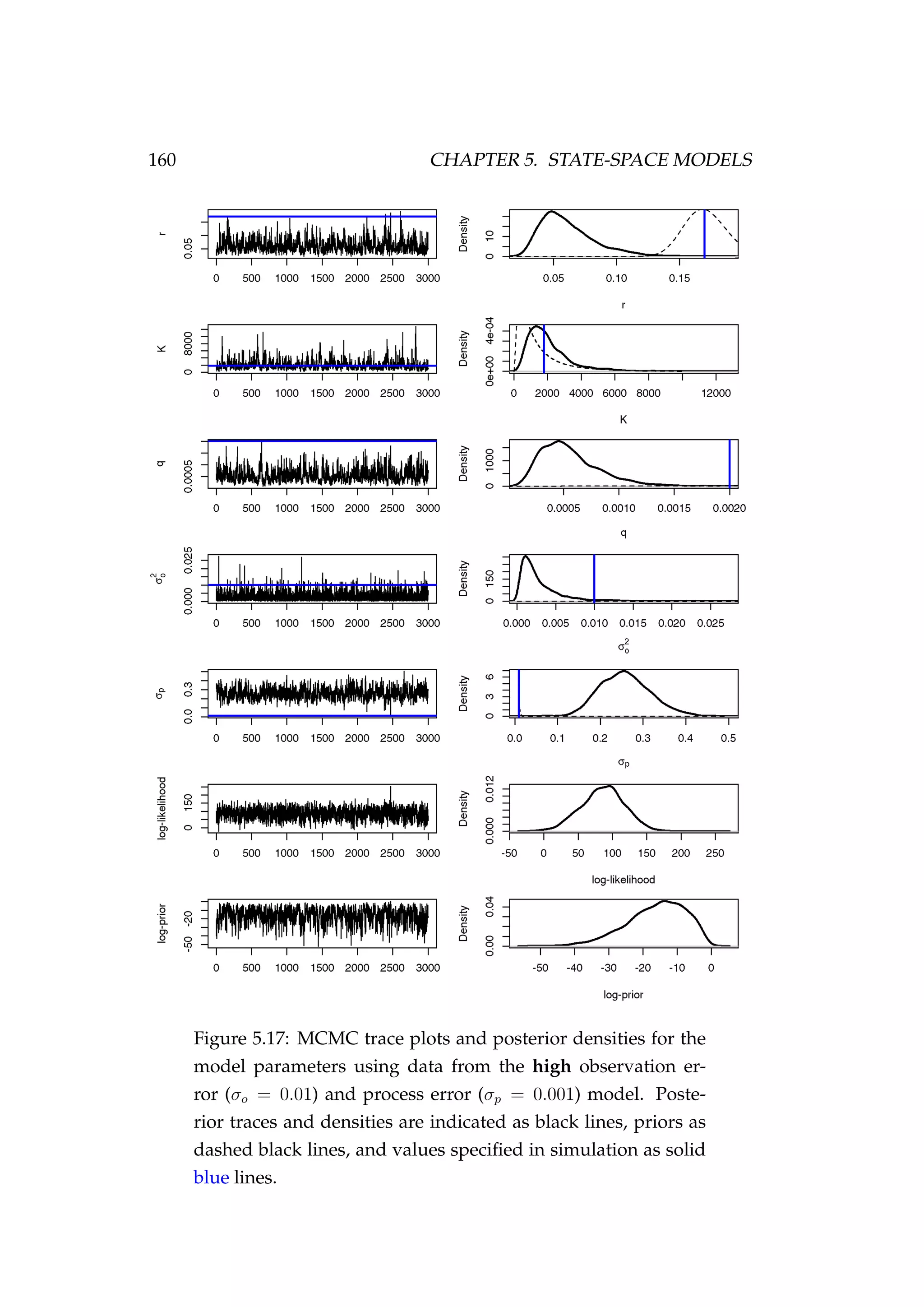
170. 158 CHAPTER 5. STATE-SPACE MODELS
the data and MCMC is simply recovering the prior. The catchability co-
efficient (q) was underestimated and the carrying capacity (K) overesti-
mated. While the model fit to the CPUE observations (It) looks adequate,
the biomass (Bt) is consistently overestimated (Figure 5.16). The fit is no
Figure 5.16: Fit to CPUE observations (It) [left] and the poste-
rior distribution of biomass (Bt) [right] for the high observa-
tion error (σp = 0.01) and process error (σp = 0.001) model es-
timated using uninformative priors for observation error vari-
ance and process error standard deviation. CPUE observations
are shown as black points [•] and the posterior distribution of
the fit to CPUE is shown in blue. The posterior distribution of
biomass is shown in green and the simulated biomass as the
dashed black line. The shading indicates the 5th, 25th, 50th,
75th and 95th percentiles.
worse than in the previous section using informative priors for σ2
o and σp
(Figure 5.12).
A naive final run
Finally, we do one last run fitting to the high observation and process error
model (σo = 0.1, σp = 0.01) only. We specifying an inverse gamma prior

171. 5.3. BIOMASS DYNAMICS STATE-SPACE MODELS 159
distribution with high variance for the process error standard deviation
(σp) and a less informative prior on the intrinsic rate of population increase
(r). The full list of priors is
π(r) ∼ log N(log(0.17), 0.2),
π(K) ∼ log N(6.90776, 0.989933),
π(q) ∼ log N(−3.45388, 1.4849),
π(σ2
o) ∼ IG(0.001, 0.001),
π(σp) ∼ IG(0.001, 0.001). (5.17)
Most parameters were not well recovered (Figure 5.17). The observation
error variance (σ2
o) was severely underestimated, while the standard devi-
ation of process error (σ2
p) was overestimated. The catchability coefficient
(q) was underestimated, as was the intrinsic rate of population increase (r).
Due to the extremely low estimates of observation error, the model fits the
CPUE observations (It) too well, resulting in unrealistic biomass estimates
(Bt, Figure 5.18).
This final model illustrates some of the difficulties faced when trying to
tease apart observation and process error in the face of uncertainty. Esti-
mating parameters relating to observation error (e.g. σ2
o) and process error
(e.g. σ2
p) simultaneously is difficult due to the anti-correlation of these (and
other) parameters (Figure 5.19).
To summarise, estimating parameters based on simulated populations
with low observation and process errors is relatively easy. However, when
faced with uncertainty, the choice of prior distributions becomes impor-
tant. Of particular importance is the choice of prior controlling the magni-
tude of process error in these types of models. When tight, highly informa-
tive, priors are used, the MCMC method performs well and parameter es-
timation is straightforward. However, it is unrealistic to expect this degree
of prior knowledge in practice. A further issue is the severe confounding
between the models key parameters r, K and q (Hilborn & Walters 1992).
However, this is largely overcome with the transformation suggested on
page 5.3.1. The key problem with these models is their inability to separate
the variance into the observation (σ2
o) and process (σ2
p) error components.

172. 160 CHAPTER 5. STATE-SPACE MODELS
Figure 5.17: MCMC trace plots and posterior densities for the
model parameters using data from the high observation er-
ror (σo = 0.01) and process error (σp = 0.001) model. Poste-
rior traces and densities are indicated as black lines, priors as
dashed black lines, and values specified in simulation as solid
blue lines.

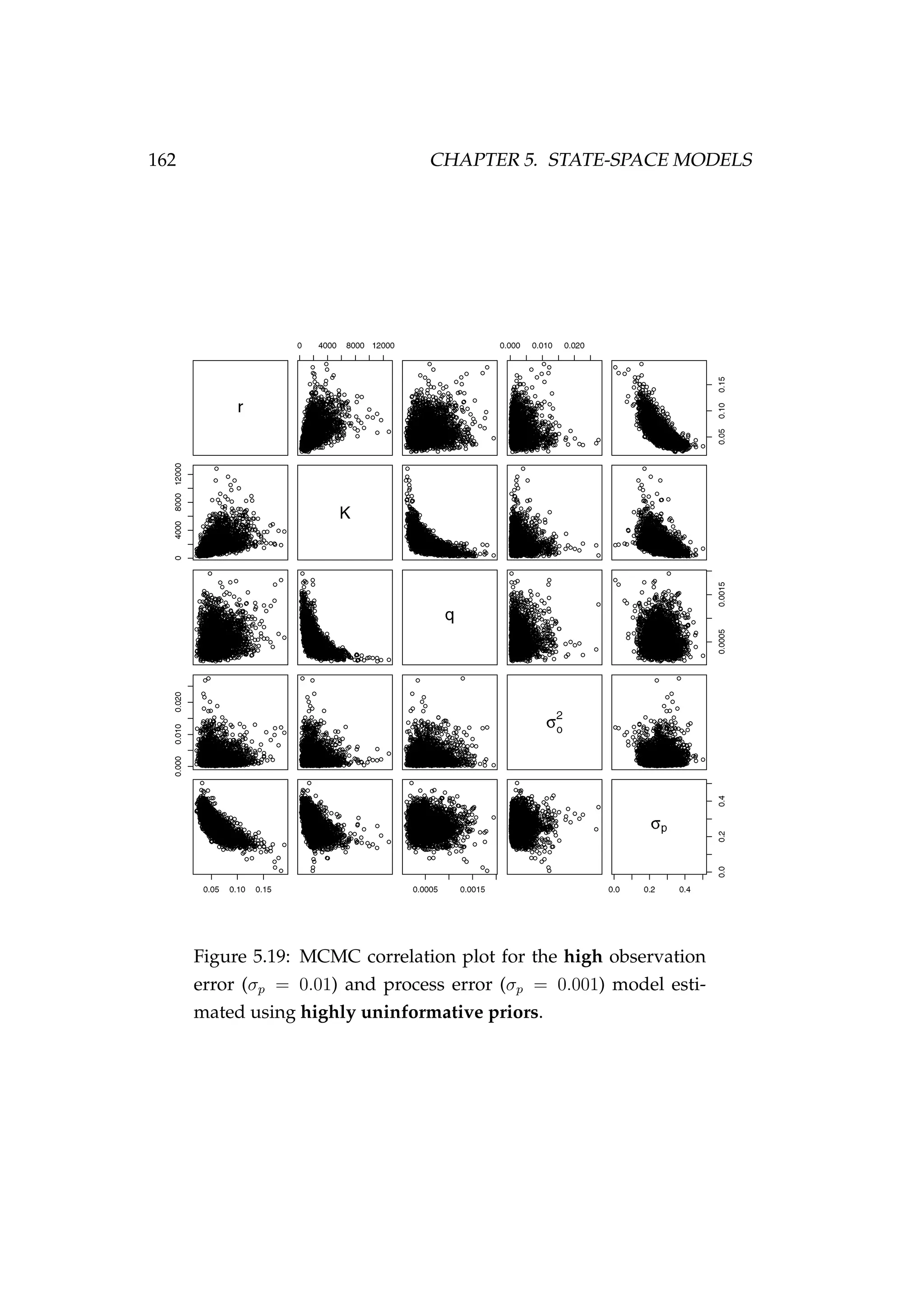
173. 5.3. BIOMASS DYNAMICS STATE-SPACE MODELS 161
Figure 5.18: Fit to CPUE observations (It) [left] and the poste-
rior distribution of biomass (Bt) [right] for the high observa-
tion error (σp = 0.01) and process error (σp = 0.001) model esti-
mated using highly uninformative priors. CPUE observations
are shown as black points [•] and the posterior distribution of
the fit to CPUE is shown in blue. The posterior distribution of
biomass is shown in green and the simulated biomass as the
dashed black line. The shading indicates the 5th, 25th, 50th,
75th and 95th percentiles.

174. 162 CHAPTER 5. STATE-SPACE MODELS
Figure 5.19: MCMC correlation plot for the high observation
error (σp = 0.01) and process error (σp = 0.001) model esti-
mated using highly uninformative priors.

175. 5.4. AGE-STRUCTURED STATE-SPACE MODELS 163
This problem arises largely due to the anti-correlation between the two
parameters (i.e. an increase in σ2
o can be compensated for by a decrease in
σ2
p during MCMC). This is a well known problem in these types of models
(see chapter 7 of Hilborn & Mangel 1997) and it is usually recommended
that we must specify the variance of either the observation error or the
process error, or the ratio of the variances (Schnute 1987). It has also been
suggested that alternative methods of inference to MCMC (i.e. sample im-
portance algorithms) can sometimes perform better here, but still do not
solve the problem entirely (pers. comm. M. McAllister). However, this
is beyond the scope of this thesis as sample importance methods are slow
when sampling high dimensional models.
5.4 Age-structured state-space models
State-space features are commonly included in age-structured stock as-
sessment models via the year class strengths (YCSt). However, the state-
space concept is rarely (if at all) applied across all ages and all years within
age-structured models. The worry might be that trying to estimate all of
the model parameters within an age-structured model along with a la-
tent state for every single age in every single year might be intractable or
take a very long time to converge. Here we attempt to make this problem
more tractable by splitting the likelihood up into components and using a
blockwise Metropolis-Hasting MCMC algorithm to try speed up MCMC
convergence.
First we define the stock’s average recruitment (R0), the stock recruitment
function (SR (SSBt)), the spawning stock biomass (SSBt, tonnes), the nat-
ural mortality at age a and time t (Ma,t), the mean weight (tonnes) of a
fish of age a during time t (wa,t), the time-varying selectivity of the fish-
ery (Sa,t), the vulnerable biomass (Va,t, tonnes), the observed catch (Ca,t,
tonnes), and the exploitation rate (Ua,t). The numbers of fish at age and
time (Na,t) in a fully state-space age-structured model (referring back to
Equation 1.26 in Chapter 1, page 42) from the beginning of the year could

176. 164 CHAPTER 5. STATE-SPACE MODELS
evolve as follows
Na,t = Na−1,t−1 ageing,
N1,t = R0 × SR (SSBt−1) × eεR
t −σ2
R/2
recruitment,
Na,t = Na,te−0.5Ma,t+εp1
a,t−σ2
p/2
half natural mortality,
SSBt =
a
Na,twa,tma,teεw
a,t−σ2
w/2+εm
a,t−σ2
m/2
spawning stock biomass,
Va,t = Na,twa,tSa,teεw
a,t−σ2
w/2+εs
a,t−σ2
s /2
vulnerable biomass,
Ua,t =
Ca,teεc
a,t−σ2
c /2
Va,t
fishing exploitation,
Ia,t = qVa,teεo
a,t−σ2
o/2
catch per unit effort,
λa,t = Na,tSa,t,
(Qa)t =
λa,t
a λa,t
where
a
(Qa)t = 1 ∀t,
(Pa)t ∼ Dirichlet (α0αa,t(Qa)t) where
a
(Pa)t = 1 ∀t proportions at age,
Na,t = Na,t 1 − Ua,tSa,teεs
a,t−σ2
s /2
fishing,
Na,t = Na,te−0.5Ma,tεp2
a,t−σ2
p/2
half natural mortality,
where we have log-normal error (indicated above in red) associated with
recruitment (εR
t ), natural mortality at age when it is applied each time (εp1
a,t
and εp2
a,t), weight at age (εw
a,t), maturity at age (εm
a,t), selectivity at age (εs
a,t),
the catch at age (εc
a,t), and the catch per unit effort (εo
a,t)
εR
t
iid
∼ N(0, σ2
R) εp1
a,t
iid
∼ N(0, σ2
p),
εw
a,t
iid
∼ N(0, σ2
w) εm
a,t
iid
∼ N(0, σ2
m),
εc
a,t
iid
∼ N(0, σ2
c ) εs
a,t
iid
∼ N(0, σ2
s ),
εp2
a,t
iid
∼ N(0, σ2
p) εo
a,t ∼ N 0, σ2
o .
We use the notation (Pa)t to make it clear that we are talking about pro-
portions in the catch at age composition Pa each year t.
In fisheries science the scaled multinomial distribution is commonly
used to fit age or length composition data (i.e. proportions in the catch

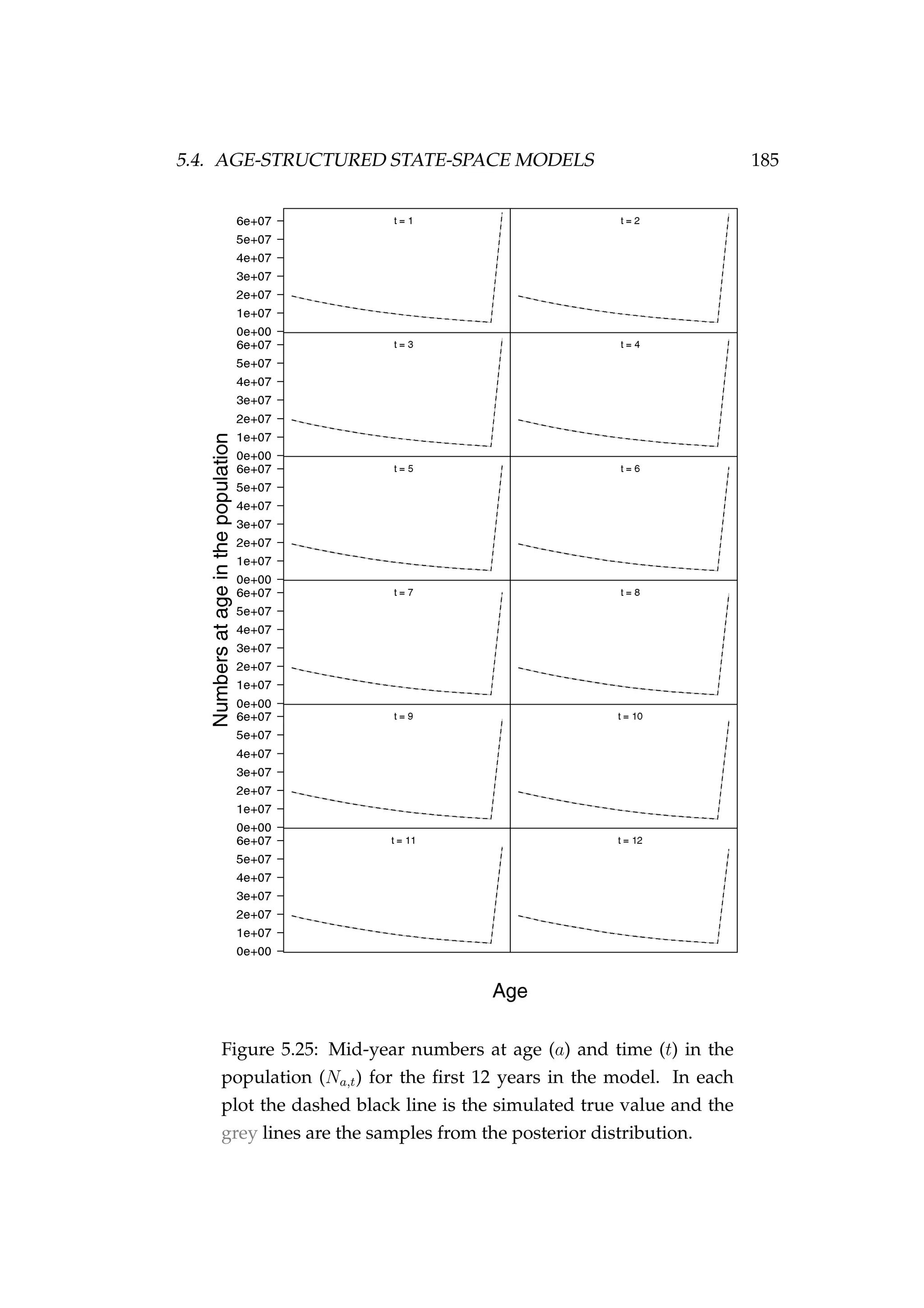
177. 5.4. AGE-STRUCTURED STATE-SPACE MODELS 165
at age, proportions at age in the population, or proportions at length,
sometimes by sex). The multinomial distribution is a generalisation of
the binomial distribution and has parameters n (the integer number of
trials n > 0) and p1, . . . , pk where k
j pj = 1
yj ∼ Multinomial(n, pj)/n,
E[yj] = pj,
V[yj] =
pj(1 − pj)
n
,
with discrete support yj ∈ {0, 1
n
, 2
n
, . . . , 1} where yj = 1. In fish-
eries science, the parameter n is derived as the number of fish in the
sample for which ages are measured, or the number of hauls in a year,
or some combination of factors that relates to the amount of sampling
done. Alternatively one might bootstrap re-sample length-frequency
distributions and an age-length key to come up with some measure of
the variance between proportions in the catch at age by year ((Pa)t).
These variances would then be used to derive an effective n (scaled by
the relative variance in each year).
However, a similar modelling approach is possible using the Dirichlet
distribution with the advantage that the distribution has continuous
support. The Dirichlet distribution is the multivariate generalisation of
the beta distribution. It has concentration parameters α1, . . . , αk, where
αj > 0 and continuous support yj ∈ [0, 1] and k
j=1 yj = 1
yj ∼ Dirichlet(α0αj),
E[yj] = αj = pj where
j
αj = 1,
V[yj] =
αj(1 − αj)
(α0 + 1)
.
Here the parameter α0 is analogous to the n parameter in a multino-
mial distribution. Small values of α0 will result in a “sloppy” (high
variance) distribution, while a large α0 will result in the expected value
of yj strongly concentrated towards pj.

178. 166 CHAPTER 5. STATE-SPACE MODELS
The Dirichlet distribution is a proper self-weighting distribution de-
signed for continuous composition data. It has been shown that the
multinomial distribution is in fact a bad choice for composition data,
despite being the most commonly used distribution for composition
data in fisheries science (Francis 2014). The multinomial distribution is
not considered further in this thesis.
In practice, this model must be greatly simplified to make inference
tractable. The reduced model that is commonly used for stock assessment
in New Zealand is
Na,t = Na−1,t−1,
N1,t = R0 × SR (SSBt−1) × eεR
t −σ2
R/2
where εR
t
iid
∼ N(0, σ2
R)
Na,t = Na,te−0.5M
,
SSBt =
a
Na,twama,
Vt =
a
Na,twaSa,
Ut =
Ct
Vt
,
It = qVteεo
t −σ2
o/2
where εo
t
iid
∼ N(0, σ2
o),
λa,t = Na,tSa,
(Qa)t =
λa,t
a λa,t
where
a
(Qa)t = 1 ∀t,
(Pa)t ∼ Multinomial (n, (Qa)t) where
a
(Pa)t = 1 ∀t,
Na,t = Na,t (1 − UtSa) ,
Na,t = Na,te−0.5M
.
This model includes log-normal recruitment error (εR
t ) and observation
error (εo
t ) only1
, ignoring any error associated with the natural mortality,
weight at age, maturity at age, selectivity at age, or catch at age. This
1
Actually, often the magnitude of observation error (a coefficient of variation) each
year for the catch per unit effort time series is calculated outside of the model and in-
cluded as a covariate. Sometimes some additional error is estimated as well.

179. 5.4. AGE-STRUCTURED STATE-SPACE MODELS 167
model also assumes that natural mortality (M) is the same for all ages
and years (rather than Ma,t, Ma or Mt), wa rather than wa,t, Sa rather than
Sa,t which results in the deconstruction of Ua,t into UtSa (see Chapter 1,
page 40). Many of these assumptions are necessary if we are to have stable
models with MCMC samplers that converge within our lifetime.
In this model Na,t are the mid-year numbers at age. Alternatively, the
numbers at age from mid-year to mid-year can be written
Na,t = Na−1,t−1e−0.5M
(1 − UtSa) e−0.5M
.
From now on we drop the notation and any reference to numbers at age
is during the middle of the year unless specified otherwise.
Now, we describe a different model that includes process error in the mid-
year numbers at age. Firstly, the weight at age (wa), maturity at age (ma)
and selectivity at age (Sa) are all calculated as
wa = w∞ 1 − e−k(a−t0) β
where w∞ = αL∞
β
, (5.18)
ma = 1 1 + 19(A50−a)/Ato95
, (5.19)
Sa = 1 1 + 19(γ50−a)/γ95
, (5.20)
where fixed parameters are indicated in blue and estimated parameters
in red. Equations 5.19 and 5.20 are logistic curves describing maturity
and selectivity at age. See Sections 1.3.2, 1.3.3 and 1.3.9 in Chapter 1 for
descriptions of each of these equations.
The deterministic equilibrium numbers at age in the population at the be-
ginning of time t = 0 (i.e. before the first year of the model) are calculated
as
N0
a =



R0e−(a−1)M
if a = 1, . . . , A
R0
eM−AM
1−e−M if a = A
,
referring back to Equation 1.19 on page 33. From this B0 is calculated mid-
year as
B0 =
a
N0
a wamae−0.5M
.
The mid-year numbers at age at time t = 1 is calculated by removing half

180. 168 CHAPTER 5. STATE-SPACE MODELS
of the total annual natural mortality (M) and adding process error (εp
a,t)
Na,t=1 = N0
a e−0.5M+εp
a,t−σ2
a,t/2
=



R0e−(a−0.5)M+εp
a,t−σ2
a,t/2
if a = 1, . . . , A
R0
eM−AM
1−e−M e−0.5M+εp
a,t−σ2
a,t/2
if a = A
,
where
εp
a,t
iid
∼ N 0, σ2
a,t ,
noticing that the process error (εp
a,t) and process error variance (σ2
a,t) are
age and time specific (discussed below). Recruitment to the population
each year (Rt) is defined as
Rt =



R0e−0.5M+εp
a,t−σ2
a,t/2
if a = 1, t = 1
R0 × SR(SSBt−1) × e−0.5M+εp
a,t−σ2
a,t/2
if a = 1, t = 2, . . . , T
,
noting that we continue to use process error terms (εp
a,t and σ2
a,t) rather
than the standard recruitment variation (σ2
R) and recruitment deviation
(εR
t ) or year class strength (YCSt) notation, this is discussed further below.
Finally, the numbers of fish transitioning between ages and years is
Na,t =



Na−1,t−1e−0.5M
(1 − Ut−1Sa−1)e−0.5M+εp
a,t−σ2
a,t/2
if a = 2, . . . , A, t = 2, . . . , T
Na−1,t−1e−0.5M
(1 − Ut−1Sa−1)e−0.5M+εp
a,t−σ2
a,t/2
+NA,t−1e−0.5M
(1 − Ut−1SA)e−0.5M+εp
a,t−σ2
a,t/2
if a = A, t = 2, . . . , T
,
where the bottom half of this equation describes the numbers at age in the
plus group. Drawing the above definitions together, the mid-year num-
bers at age in the population (Na,t) at all ages and all times can be sum-
marised as
Na,t =



R0e−0.5M+εp
a,t−σ2
a,t/2
if a = 1, t = 1
R0e−(a−0.5)M+εp
a,t−σ2
a,t/2
if a = 2, . . . , A, t = 1
R0
eM−AM
1−e−M e−0.5M+εp
a,t−σ2
a,t/2
if a = A, t = 1
R0 × SR(SSBt−1) × e−0.5M+εp
a,t−σ2
a,t/2
if a = 1, t = 2, . . . , T
Na−1,t−1e−0.5M
(1 − Ut−1Sa−1)e−0.5M+εp
a,t−σ2
a,t/2
if a = 2, . . . , A, t = 2, . . . , T
Na−1,t−1e−0.5M
(1 − Ut−1Sa−1)e−0.5M+εp
a,t−σ2
a,t/2
+NA,t−1e−0.5M
(1 − Ut−1SA)e−0.5M+εp
a,t−σ2
a,t/2
if a = A, t = 2, . . . , T
.
(5.21)

181. 5.4. AGE-STRUCTURED STATE-SPACE MODELS 169
Given the mid-year numbers at each age a and at each time t we can derive
the following standard quantities
SSBt =
a
Na,twama, (5.22)
SR(SSBt) =
SSBt
B0
1 −
5h − 1
4h
1 −
SSBt
B0
, (5.23)
Vt =
a
Na,twaSa, (5.24)
Ut =
Ct
Vt
, (5.25)
It = qVteεo
t −σ2
o/2
where εo
t ∼ N 0, σ2
o , (5.26)
λa,t = Na,tSa,
(Qa)t =
λa,t
a λa,t a
(Qa)t = 1 ∀t,
(Pa)t ∼ Dirichlet (α0αt(Qa)t)
a
(Pa)t = 1 ∀t, (5.27)
where estimated parameters, latent states, and functions arising from esti-
mated parameters are indicated in red. Fixed parameters, covariates, and
functions arising from fixed parameters are indicated in blue. Observa-
tions are indicated in green. The CPUE (It) is assumed to be log-normally
distributed and the proportions in the catch at age ((Pa)t) are assumed to
be Dirichlet distributed. Here, the Dirichlet distribution uses an annual
scaling covariate (αt) that is used to define the relative weight of propor-
tions in the catch at age ((Pa)t) between years. The values of these covari-
ates are assumed known and could be estimated outside of the stock as-
sessment model, much like an effective n is estimated for the multinomial
distribution. The estimated parameter α0 scales αt(Qa)t and is analogous
to data weighting within the model. For a thorough discussion on data
weighting in stock assessment see Francis (2011). Also see the discussion
at the end of this chapter (page 204).
The variance of the process error in this model is defined as an A×T matrix

182. 170 CHAPTER 5. STATE-SPACE MODELS
for convenience, i.e. specifying a process error for each age and time
σ2
a,t =






σ2
R σ2
R · · · σ2
R
σ2
R σ2
p · · · σ2
p
...
...
...
...
σ2
R σ2
p · · · σ2
p






A×T
. (5.28)
Here we have specified two process error variance parameters, variance
associated with recruitment and numbers at age in the first year (σ2
R), and
the variance associated with all other transitions (σ2
p, Figure 5.20). Con-
R0 R0 × SR(SSBt−1)
N0
a
...
N0
a
N0
A
a = 1
a = A
t = 1 t = T
σ2
p
σ2
p
σ2
p
σ2
p
σ2
p
σ2
p
σ2
p
σ2
p
σ2
p
σ2
p
σ2
p
σ2
p
σ2
p
σ2
p
σ2
p
σ2
p
σ2
p
σ2
p
σ2
p
σ2
p
σ2
p
σ2
p
σ2
p
σ2
p
σ2
p
σ2
p
σ2
p
σ2
p
σ2
p
σ2
p
σ2
p
σ2
p
σ2
p
σ2
p
σ2
p
σ2
p
σ2
p
σ2
p
σ2
p
σ2
p
σ2
p
σ2
p
σ2
p
σ2
p
σ2
p
σ2
p
σ2
p
σ2
p
σ2
p
σ2
R
σ2
R
σ2
R
σ2
R
σ2
R
σ2
R
σ2
R
σ2
R σ2
R σ2
R σ2
R σ2
R σ2
R σ2
R σ2
R
Figure 5.20: Matrix showing the direction of transitions be-
tween numbers of fish at age and time (Na,t) within the model
and the process errors variance to be used at each age a and
time t. The numbers of fish for all ages and all times is defined
by Equation 5.21. The colours are used to highlight the 6 parts
of Equation 5.21.
sequently, the year class strengths (YCSt) for each year can be calculated

183. 5.4. AGE-STRUCTURED STATE-SPACE MODELS 171
as
YCSt = eεp
a=1,t−σ2
a=1,t/2
= eεp
a=1,t−σ2
R/2
∀t. (5.29)
In summary, this model makes the following assumptions:
• the natural mortality rate (M), the maturity parameters (A50 and
Ato95), the von Bertalanffy growth parameters (L∞, k and t0) and the
length-weight parameters (α and β) are all known parameters (ω)
• natural mortality (M) is constant over age a and time t (Ma,t = M)
• mean weight is deterministic (i.e. without error) and constant over
time (wa,t = wa)
• selectivity is deterministic (i.e. without error) and constant over time
(Sa,t = Sa)
• catch (Ct) is measured without error
• the exploitation rate (Ut) is constant by age (Ua,t = Ut)
• CPUE (It) is proportional to abundance.
• the population is closed (no immigration or emigration)
• the numbers at age at the start of the model are log-normally dis-
tributed about N0
a with variance σ2
R (Equation 5.21)2
.
5.4.1 Inference
We are interested in attaining a probabilistic relationship between the fol-
lowing:
• The data y: the catch per unit effort (It) and proportions in the catch
at age (Pa,t). Let y = {{It}T
t=1, {{Pa,t}A
a=1}T
t=1}
2
Here σ2
p could be used rather than σ2
R. This would assume that the age composi-
tion at the beginning of the model is more similar to the equilibrium numbers at age.
Composition data that enables us to estimate these year classes are rarely available in
the early years of stock assessment models so this mat be a better choice in many cases.
Alternatively, an entirely different variance parameter (e.g. σ2
N ) could be estimated.

184. 172 CHAPTER 5. STATE-SPACE MODELS
• The covariates z: the catch (Ct) and the relative variances (weights)
of the Dirichlet distribution for the proportions in the catch at age
data (αt). Let z = {Ct, αt}T
t=1
• The unknown parameters of interest θ: the virgin recruitment (R0)
and the selectivity parameters (γ50 and γ95). Let θ = {R0, γ50, γ95}
• The unknown nuisance parameters φ: the catchability coefficient
(q), the observation error variance (σ2
o), the process error variance
(σ2
p), the recruitment deviation variance (σ2
R), and the scaling of the
Dirichlet distribution variances (α0). Let φ = {q, σ2
o, σ2
p, σ2
R, α0}
• The known parameters ω: the natural mortality rate (M), the matu-
rity parameters (A50 and Ato95), the von Bertalanffy growth parame-
ters (L∞, k and t0) and the length-weight parameters (α and β). Let
ω = {M, h, A50, Ato95, L∞, k, t0, α, β}
• The unknown latent states x: the numbers at age during the mid-
dle of the year (Na,t, i.e. after half of the natural mortality has been
applied, but before fishing). Let x = {Na,t}A,T
a=1,t=1
Using Bayes theorem, the posterior distribution of the model parameters
(θ and φ) and states (x), given the fixed parameters (ω), data (y) and co-
variates (z) is
π(θ, φ, x|ω, y, z) ∝ π(θ, φ, x|ω, z)π(y|θ, φ, ω, x, z), (5.30)

185. 5.4. AGE-STRUCTURED STATE-SPACE MODELS 173
where the prior is
π(θ, φ, x|ω, z) = π(R0, γ50, γ95, q, σ2
o, σ2
p, σ2
R, α0, x|ω, z)
= π(R0)π(γ50)π(γ95)π(q)π(σ2
o)π(σ2
p)π(σ2
R)π(α0)π(x|θ, φ, ω, z)
= π(R0)π(γ50)π(γ95)π(q)π(σ2
o)π(σ2
p)π(σ2
R)π(α0)
×
T
t=1
π Na=1,t|R0, SSBt−1, σ2
R, ω
×
A
a=1
π Na,t=1|R0, σ2
R, ω
×
A−1
a=2
T
t=2
π Na,t|Na−1,t−1, Vt−1, Ct−1, γ50, γ95, σ2
p, ω ,
×
T
t=2
π Na=A,t|NA−1,t−1, NA,t−1, Vt−1, Ct−1, γ50, γ95, σ2
p, ω ,
and the likelihood is
π (y|θ, φ, ω, x, z) = π I, P|γ50, γ95, q, σ2
o, α0, ω, x, z
= π(I|γ50, γ95, q, σ2
o, x)π(P|γ50, γ95, α0, x, z, ω)
=
T
t=1
π(It|Na,t, γ50, γ95, q, σ2
o, ω)
×
A
a=1
T
t=1
π ((Pa)t|Na,t, Ct, αt, γ50, γ95, α0, ω) .
The likelihood of this model is made up of three main components: the
likelihood of the CPUE observations (It), the likelihood of the proportions
in the catch at age observations ((Pa)t), and the likelihood of the numbers
at age latent states (Na,t). The likelihood of the CPUE observations is
log (It) |Na,t, γ50, γ95, q, σ2
o, ω, ∼ N log (qVt) − σ2
o/2, σ2
o . (5.31)
The likelihood of the proportions in the catch at age is
(Pa)t|Na,t, Ct, αt, γ50, γ95, α0, ω ∼ Dirichlet (α0αt(Qa)t) , (5.32)
where α0 is a scaling parameter defining the variability in the Dirichlet
distribution and αt is the annual variation. The likelihood of the numbers

186. 174 CHAPTER 5. STATE-SPACE MODELS
at age is
log (Na,t) |µa,t, Ct, γ50, γ95, σ2
a,t, ω ∼ N log (µa,t) − σ2
a,t/2, σ2
a,t , (5.33)
where
µa,t =



R0e−0.5M
if a = 1, t = 1
R0e−(a−0.5)M
if a = 2, . . . , A, t = 1
R0
eM−AM
1−e−M e−0.5M
if a = A, t = 1
R0 × SR(SSBt−1) × e−0.5M
if a = 1, t = 2, . . . , T
Na−1,t−1e−0.5M
(1 − Ut−1Sa−1)e−0.5M
if a = 2, . . . , A, t = 2, . . . , T
Na−1,t−1e−0.5M
(1 − Ut−1Sa−1)e−0.5M
+NA,t−1e−0.5M
(1 − Ut−1SA)e−0.5M
if a = A, t = 2, . . . , T
,
(5.34)
noting the similarity with Equation 5.21. Using MCMC we can sample
from the posterior distribution (Equation 5.30) to obtain probability distri-
butions of the parameters, latent states and other quantities of interest in
the model. We provide an example below (Section 5.4.2, page 179). Using
Equation 5.30 and the priors described below we estimate posterior distri-
butions for each of the parameters using blockwise Metropolis-Hastings
with log-normal proposals (see Chapter 2, page 66).
The three main components of the likelihood described above can be split
into even smaller subcomponents made up of just single ages a and years
t. When a parameter or latent state is proposed within MCMC, then only
the probability density function (PDF) of those subcomponents relevant to
the proposal, and the prior, need be evaluated. Each of the MCMC pro-
posals and the subcomponents of the likelihood for which the PDF needs
to be evaluated, excluding the priors (these are specified in the preceding
sections), are as follows:
• When proposing R∗
0 update B0 and SR(SSBt) then calculate the PDF
of
log (Na=1,t) ∼ N log (µa=1,t) , σ2
a=1,t ∀t,
log (Na,t=1) ∼ N log (µa,t=1) , σ2
a,t=1 a = 2, . . . , A.

187. 5.4. AGE-STRUCTURED STATE-SPACE MODELS 175
i.e. at age 1 and at time 1.
• When proposing q∗
calculate the PDF of
log (It) ∼ N log (q∗
Vt) , σ2
o ∀t.
• When proposing γ∗
50 or γ∗
95 update Sa, Vt, Ut, (Qa)t then calculate the
PDF of
log (It) ∼ N log (qVt) , σ2
o ∀t,
(Pa)t ∼ Dirichlet (α0αt(Qa)t) ∀t,
log (Na,t) ∼ N log (µa,t) , σ2
a,t a = 2, . . . , A, t = 2, . . . , T.
• When proposing σ2∗
o calculate the PDF of
log (It) ∼ N log (qVt) , σ2∗
o ∀t.
• When proposing σ2∗
p calculate the PDF of
log (Na,t) ∼ N log (µa,t) , σ2∗
p a = 2, . . . , A, ∀t.
• When proposing σ2∗
R calculate the PDF of
log (Na=1,t) ∼ N log (µa=1,t) , σ2∗
R ∀t.
• When proposing α∗
0 calculate the PDF of
(Pa)t ∼ Dirichlet (α∗
0αt(Qa)t) ∀a∀t,
• When proposing N∗
a,t update SSBt, SR(SSBt), Vt, Ut, (Qa)t then cal-
culate the PDF of
log (It) ∼ N log (qVt) , σ2
o ,
(Pa)t ∼ Dirichlet (α0αt(Qa)t) ,
log N∗
a,t ∼ N log (µa,t) , σ2
a,t
log (Na,t+1) ∼ N log (µa,t+1) , σ2
a,t ∀a.
See Figure 5.21 for a graphic example of the subcomponents of the
likelihood for which PDFs need to be evaluated when proposing N∗
a,t
for a single a and t.

188. 176 CHAPTER 5. STATE-SPACE MODELS
R0 R0 × SR(SSBt−1)
N0
a
...
N0
a
N0
A
a = 1
a = A
t = 1 t = T
σ2
p
σ2
p
σ2
p
σ2
p
σ2
p
σ2
p
σ2
p
σ2
p
σ2
p
σ2
p
σ2
p
σ2
p
σ2
p
σ2
p
σ2
p
σ2
p
σ2
p
σ2
p
σ2
p
σ2
p
σ2
p
σ2
p
σ2
p
σ2
p
σ2
p
σ2
p
σ2
p
σ2
p
σ2
p
σ2
p
σ2
p
σ2
p
σ2
p
σ2
p
σ2
p
σ2
p
σ2
p
σ2
p
σ2
p
σ2
p
σ2
p
σ2
p
σ2
p
σ2
p
σ2
p
σ2
p
σ2
p
σ2
p
σ2
p
σ2
R
σ2
R
σ2
R
σ2
R
σ2
R
σ2
R
σ2
R
σ2
R σ2
R σ2
R σ2
R σ2
R σ2
R σ2
R σ2
R
Figure 5.21: If updating the green cell (Na,t), then the likeli-
hood of that cell given the previous numbers at age and time
(Na−1,t−1, shown in red) and the numbers at all ages in the fol-
lowing time step (Na,t+1 ∀a, shown in red) need to be evaluated.
The probability of the numbers at age for time t + 1 need to be
evaluated as they depend on variables derived from the num-
bers in the previous time step t, namely the spawning stock
biomass (SSBt), the stock recruitment (SR(SSBt )), the vulnera-
ble biomass (Vt) and the exploitation rate (Ut).

189. 5.4. AGE-STRUCTURED STATE-SPACE MODELS 177
One of the greatest challenges in MCMC is achieving good mixing of the
chains. When simultaneously sampling a large number of parameters (i.e.
multivariate proposals), the algorithm might find it difficult to achieve
good mixing as multiple parameter updates can be difficult to construct
and tune. On the other hand, single parameter updates can result in slow
mixing, if the proposal variance is low, many proposals are accepted, but
mixing is slow. If the proposal variance is high, many proposals are re-
jected. In practice it is often a good idea to form small groups of corre-
lated parameters that belong to the same context in the formulation of the
model. The best mixing is usually obtained with a blocking strategy some-
where between the all-at-once and one-at-a-time strategies.
Initial exploration suggested that mixing of the numbers at age latent
states (Na,t) was very slow. This is likely to be due to the high correlation
between numbers at age and time within cohorts (i.e. Na,t and Na+1,t+1
are highly correlated). Rather than using a multivariate proposal distribu-
tion, we developed a proposal that updates a diagonal block of numbers
at age (i.e. a cohort) by scaling the entire cohort up or down. This diago-
nal cohort update is achieved by drawing a scaling parameter (λ∗
) from a
log-normal distribution
λ∗
∼ log N 0, σ2
q . (5.35)
We define each cohort as a vector ηi where there are i = 1, . . . , k cohorts in
the model and ηi = {ηj}p
j=1 and we have j = 1, . . . , p age classes within a
cohort. We then scale a cohort i using
η∗
i,j = ηi,jλ∗
i . (5.36)
Now we derive the proposal ratio for this move, we write
η∗
i,j = ηi,jλ∗
i υ∗
j forwards move,
ηi,j = η∗
i,jλiυj reverse move,

190. 178 CHAPTER 5. STATE-SPACE MODELS
and show that
η∗
i,j = η∗
i,jλiυjλ∗
i υ∗
j
= η∗
i,jλiλ∗
i υjυ∗
j
1 = λiλ∗
i υjυ∗
j = λiλ∗
i
λi =
1
λ∗
i
,
log λi = − log λ∗
i ,
where υj = {υj}p
j=1 and
λ∗
i ∼ log N 0, σ2
λ ,
υ∗
j
iid
∼ log N 0, σ2
υ ∀j,
∂η∗
i,j
∂υ∗
j
= ηi,jλ∗
i .
The proposal density for a single cohort is
q η∗
i,j, λ∗
i |ηi,j, λi = q η∗
i,j|λ∗
i , ηi,j, λi q (λ∗
i |ηi,j, λi) ,
= q υ∗
j |λ∗
i , ηi,j, λi
∂υ∗
j
∂η∗
i,j
q (λ∗
i |ηi,j, λi) ,
=
p
j
1
υ∗
j
2πσ2
υ
−1
2
e
− 1
2σ2
υ
(log υ∗
j )2 1
ηi,jλ∗
i
2πσ2
λ
−1
2
e
− 1
2σ2
λ
(log λ∗
i )2
= 2πσ2
υ
−1
2
2πσ2
λ
−1
2
p
j
1
ηi,jλ∗
i e
− 1
2σ2
υ
(log υ∗
j )2
1
λ∗
i
e
− 1
2σ2
λ
(log λ∗
i )2
,

191. 5.4. AGE-STRUCTURED STATE-SPACE MODELS 179
therefore the proposal ratio is
q ηi,j, λi|η∗
i,j, λ∗
i
q η∗
i,j, λ∗
i |ηi,j, λi
=
p
j
1
η∗
i,jλi
e
− 1
2σ2
υ
(log υj)2
p
j
1
ηi,jλ∗
i
e
− 1
2σ2
υ
(log υ∗
j )2
×
1
λi
e
− 1
2σ2
λ
(log λi)2
1
λ∗
i
e
− 1
2σ2
λ
(log λ∗
i )2
=
p
j
ηi,jλ∗
i
η∗
i,jλi
e
− 1
2σ2
υ
((log υj)2−(log υ∗
j )2
)
×
λ∗
i
λi
× e
− 1
2σ2
λ
((log λi)2−(log λ∗
i )2
)
if συ ← 0 then υj ← 1 therefore
=
p
j
η∗
i,jλiλ∗
i
η∗
i,jλi
λ∗
i
λi
=
p
j
η∗
i,jλiλ∗
i
η∗
i,jλi
(λ∗
i )2
= (λ∗
i )p+2
.
5.4.2 Snapper simulation example
In the following sections we present three examples in which we simulate
data based loosely on the snapper (Pagurus auratus) fishery in northern
New Zealand (see Chapter 3, page 77). For most parameters we use a set
of plausible values in each example. In these examples the only parameter
that is altered is the recruitment variance parameter in the third example
(σ2
R).
In all simulations the ages modelled are a = 1, . . . , A where A is a plus
group at 20 years of age. The actual catch history of the snapper fishery
(aggregated to a single area) is used in all simulation runs (Figure 5.22). We
cut down the number of years modelled in this simulation to 100 (from
114, purely for ease of presenting outputs). In summary, this is a single
area, single sex, single fishery, age-structured model with 20 age categories
(A = 20) and 100 time-steps or years (T = 100).
In each example, we fit the fully state-space age-structured model using
different priors for each of the models key parameters. We then attempt to

192. 180 CHAPTER 5. STATE-SPACE MODELS
Figure 5.22: Actual catch history (tonnes) of the snapper fishery
(SNA 1) from 1900 to 2013 (114 years) used in the simulation.
sample from the posterior distribution using MCMC. In the first example,
all of the key model parameters are fixed and only the numbers at age and
time latent states (Na,t) are estimated. In the remaining two examples, all
key parameters but the process error variance (σ2
p) are estimated. Addi-
tional MCMC diagnostic plots for each of the examples presented below
are provided in Appendix B.
Model validation
The first example simulates data using the model parameters shown in
Table 5.2. Notice that the recruitment variance (σ2
R) parameter is set at
a very low value. We come back to a discussion of this important and
highly influential parameter in Section 5.4.2 (page 201) below and in the
discussion at the end of this chapter (page 204).
We began by fixing all of the key model parameters to their true val-
ues during estimation (i.e. the values specified in Table 5.2) and ran the
MCMC to obtain posterior distributions of the numbers at age latent states
only. This example was done to ensure there were no problems in the

193. 5.4. AGE-STRUCTURED STATE-SPACE MODELS 181
Table 5.2: Parameter values used in age-structured simulation.
The parameters are grouped into estimated parameters of in-
terest (θ), nuisance parameters (φ) and fixed parameters (ω).
Parameter Value Units Description
R0 20 million - Recruitment at virgin
biomass
γ50 6.5 years Logistic selectivity
γ95 3 years Logistic selectivity
q 0.006 tonnes−1 Catchability coefficient
σ2
o 0.022 - Observation error variance
σ2
p 0.0012 - Process error variance for
a = 2, . . . , A and t = 2, . . . , T
σ2
R 0.0012 - Process error variance for
a = 1 ∀t and t = 1 ∀a
α0 1.0 - Dirichlet scaling
M 0.075 - Natural mortality rate
h 0.85 - Stock recruit steepness
A50 4 years Logistic maturity
Ato95 4.7 years Logistic maturity
L∞ 58.8 cm von Bertalanffy growth
k 0.102 years−1 von Bertalanffy growth
t0 -1.11 years von Bertalanffy growth
α 4.467e-8 - Length-weight
β 2.793 - Length-weight

194. 182 CHAPTER 5. STATE-SPACE MODELS
model specification or the MCMC sampler. Initial exploration showed that
getting the numbers at age latent states (Na,t) to mix properly was difficult,
even when the key parameters were fixed. However, by reducing the re-
cruitment variance (σ2
R) in the simulation to the low values specified above
resulted in better mixing. Including the diagonal numbers at age update
also improved mixing substantially.
Two million iterations were run using blockwise Metropolis-Hastings
with log-normal proposals (see Chapter 2, page 66). These two million
iterations were run as two separate MCMC chains on different computer
cores, both initialised with different random number seeds (the starting
values were the same though). Each chain ran an additional burn-in of
ten thousand iterations. The chains were thinned to save every 1000th
iteration. This resulted in a total of 2000 samples from the posterior dis-
tribution for each of the parameters and latent states. This MCMC took
about four days to complete.
The different components of the log-likelihood mixed well in the MCMC
sampler (Figure 5.23). The numbers at age latent states (Na,t) are reason-
ably well mixed. We provide a selection of MCMC trace plots for these
in Figure 5.24. More trace plots for the numbers at age can be found in
Appendix B.2, page 328. In most cases, the posterior density of the num-
bers at age states are centered over the simulated numbers at age and
time (Figure 5.24). When plotted against the simulated numbers at age
and time, the posterior density of the numbers at age match very closely
(Figures 5.25 and 5.26). Consequently, the model fits the CPUE (It) and
proportions in the catch at age ((Pa)t) data very well (Figures 5.27, 5.28,
and 5.29). Finally, looking at some of the derived quantities, the posterior
distribution of YCSs for each year of the model encompass the simulated
YCSs but do not show the same pattern through time that was estimated
(Figure 5.30). But, remember that the recruitment variation (σ2
R) was fixed
at a very low value so strong year classes are absent from this simulated
population making their estimation difficult. The estimated biomass (vul-
nerable, spawning stock and total) all match the simulated biomass very
well (Figure 5.30).

195. 5.4. AGE-STRUCTURED STATE-SPACE MODELS 183
Figure 5.23: MCMC trace plots [left] and density plots [right] of
the different components of the model log-likelihood including
the log-likelihood of the CPUE observations, the proportions in
the catch at age observations, the numbers at age latent states,
the prior contribution (which is fixed as all of the key parame-
ters are fixed) and the total log-likelihood. The horizontal blue
lines indicate the log-likelihood for each of the likelihood com-
ponents in the simulation given the true parameter values. All
panels are made up of two separate MCMC chains of 1000 sam-
ples initialised with different random number seeds.

196. 184 CHAPTER 5. STATE-SPACE MODELS
Figure 5.24: MCMC trace plots for some of the mid-year num-
bers at age latent states (Na,t). The age a and time t of each
latent state is given at the top of each trace plot. The simulated
number at age is shown as a solid horizontal blue line. All pan-
els are made up of two separate MCMC chains of 1000 samples
initialised with different random number seeds.

197. 5.4. AGE-STRUCTURED STATE-SPACE MODELS 185
Figure 5.25: Mid-year numbers at age (a) and time (t) in the
population (Na,t) for the first 12 years in the model. In each
plot the dashed black line is the simulated true value and the
grey lines are the samples from the posterior distribution.

198. 186 CHAPTER 5. STATE-SPACE MODELS
Figure 5.26: Mid-year numbers at age (a) and time (t) in the
population (Na,t) for the last 12 years in the model. In each plot
the dashed black line is the simulated true value and the grey
lines are the samples from the posterior distribution.

199. 5.4. AGE-STRUCTURED STATE-SPACE MODELS 187
Figure 5.27: Observed CPUE (It) [•] and samples from the pos-
terior distribution (qVt) [grey lines].
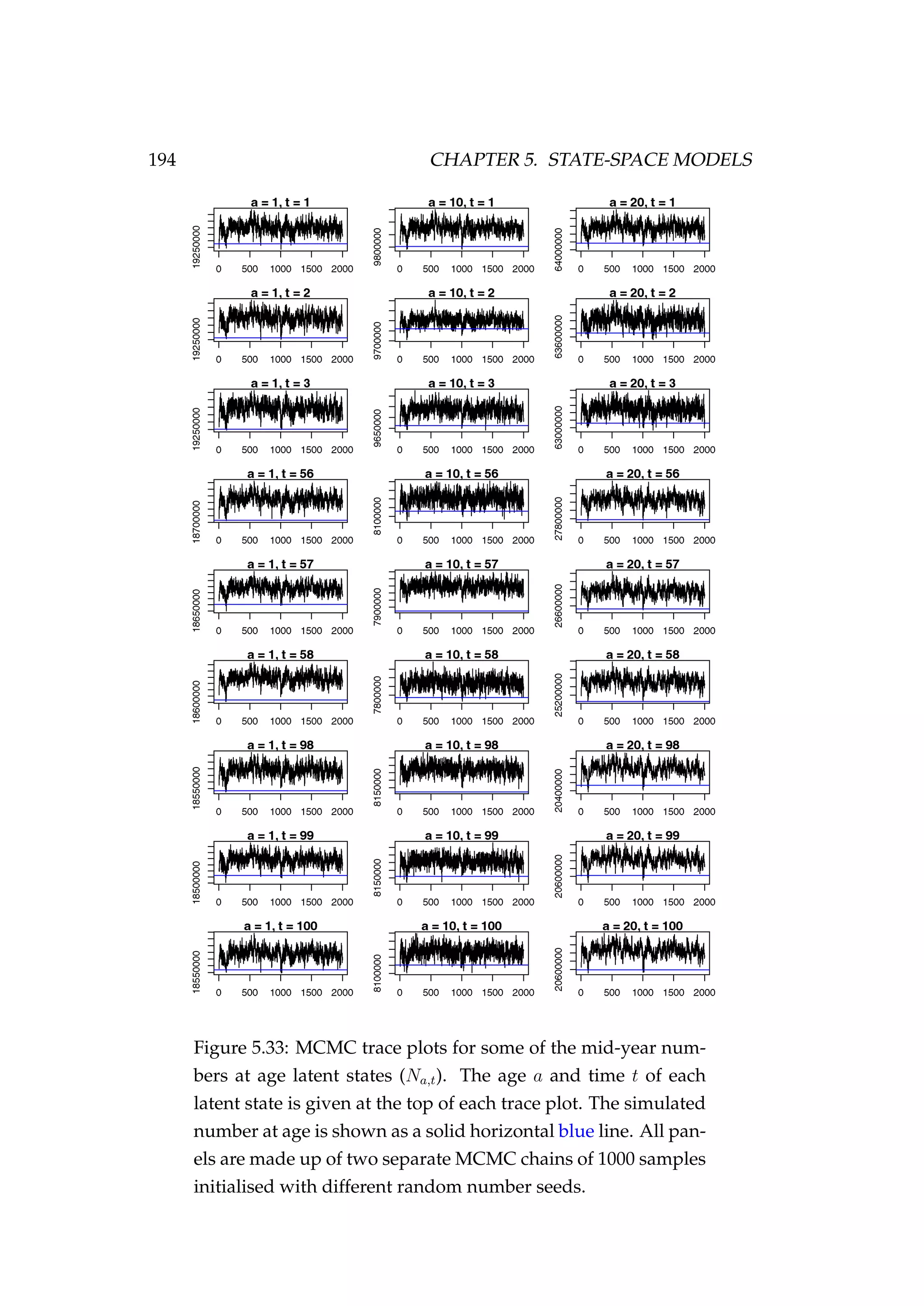
In conclusion, the model appears to be able to recover the true numbers
at age latent states reasonably well and the MCMC performance is accept-
able.

200. 188 CHAPTER 5. STATE-SPACE MODELS
Figure 5.28: Samples from the posterior distribution of the pro-
portions in the catch at age in the vulnerable portion of the
population ((Qa)t) [grey lines] and observed proportions in the
catch at age ((Pa)t) [•] for the first 12 months of the model.

201. 5.4. AGE-STRUCTURED STATE-SPACE MODELS 189
Figure 5.29: Samples from the posterior distribution of the pro-
portions in the catch at age in the vulnerable portion of the
population ((Qa)t) [grey lines] and observed proportions in the
catch at age ((Pa)t) [•] for the last 12 months of the model.

202. 190 CHAPTER 5. STATE-SPACE MODELS
Figure 5.30: Year class strengths by year (YCSt = eεp
a=1,t−σ2
R/2
)
[left], and measures of biomass in the population (including the
total biomass (Bt) in green, the spawning stock biomass (SSBt)
in red and the vulnerable biomass (Vt) in grey) [right]. In each
plot the dashed black line is the simulated true value and the
coloured lines are the samples from the posterior distribution.

203. 5.4. AGE-STRUCTURED STATE-SPACE MODELS 191
Model fit (fixed process error)
The second example uses exactly the same parameter set specified in Ta-
ble 5.2 in the simulation for this example. However, now we allow all
but one of the key parameters to be estimated. We leave the process error
variance (σ2
p) fixed and begin by specifying highly informative priors for
each of the remaining model parameters to check for any problems in the
MCMC. The full list of priors is
π(R0) ∼ log N(log(20000000), 0.005),
π(γ50) ∼ log N(log(6.5), 0.005),
π(γ95) ∼ log N(log(3), 0.005),
π(q) ∼ log N(log(0.006), 0.003),
π(σ2
o) ∼ log N(log(0.022
), 0.05),
π(σ2
R) ∼ log N(log(0.0012
), 0.05),
π(α0) ∼ log N(log(1), 0.1). (5.37)
Two million iterations were run using blockwise Metropolis-Hastings
with log-normal proposals (see Chapter 2, page 66). These three million
iterations were run as three separate MCMC chains on different computer
cores, all initialised with different random number seeds. Each chain ran
an additional burn-in of two million iterations. The chains were thinned
to save every 1000th iteration. This resulted in a total of 1000 samples of
the posterior distribution for each of the parameters and latent states.
Both the key model parameters and the different components of the log-
likelihood mixed reasonably well in the MCMC sampler (Figures 5.31
and 5.32). The numbers at age latent states (Na,t) are reasonably well
mixed. We provide a selection of MCMC trace plots for these in Fig-
ure 5.33. More trace plots for the numbers at age can be found in Ap-
pendix B.3, page 328. In most cases, the posterior density of the num-
bers at age states are centered over the simulated numbers at age and
time (Figure 5.24). When plotted against the simulated numbers at age
and time, the posterior density of the numbers at age match very closely
(Figures 5.34 and 5.35). Consequently, the model fits the CPUE (It) and

204. 192 CHAPTER 5. STATE-SPACE MODELS
Figure 5.31: MCMC trace plots [left] and posterior densities
[right] for the key model parameters. The horizontal blue lines
indicate the true parameter values as specified in the simula-
tion. All panels are made up of two separate MCMC chains of
1000 samples initialised with different random number seeds.

205. 5.4. AGE-STRUCTURED STATE-SPACE MODELS 193
Figure 5.32: MCMC trace plots [left] and density plots [right]
of the different components of the model log-likelihood includ-
ing the log-likelihood of the CPUE observations, the propor-
tions in the catch at age observations, the numbers at age latent
states, the prior contribution and the total log-likelihood. The
horizontal blue lines indicate the log-likelihood for each of the
likelihood components in the simulation given the true param-
eter values. All panels are made up of two separate MCMC
chains of 1000 samples initialised with different random num-
ber seeds.

206. 194 CHAPTER 5. STATE-SPACE MODELS
Figure 5.33: MCMC trace plots for some of the mid-year num-
bers at age latent states (Na,t). The age a and time t of each
latent state is given at the top of each trace plot. The simulated
number at age is shown as a solid horizontal blue line. All pan-
els are made up of two separate MCMC chains of 1000 samples
initialised with different random number seeds.

207. 5.4. AGE-STRUCTURED STATE-SPACE MODELS 195
Figure 5.34: Mid-year numbers at age (a) and time (t) in the
population (Na,t) for the first 12 years in the model. In each
plot the dashed black line is the simulated true value and the
grey lines are the samples from the posterior distribution.

208. 196 CHAPTER 5. STATE-SPACE MODELS
Figure 5.35: Mid-year numbers at age (a) and time (t) in the
population (Na,t) for the last 12 years in the model. In each plot
the dashed black line is the simulated true value and the grey
lines are the samples from the posterior distribution.

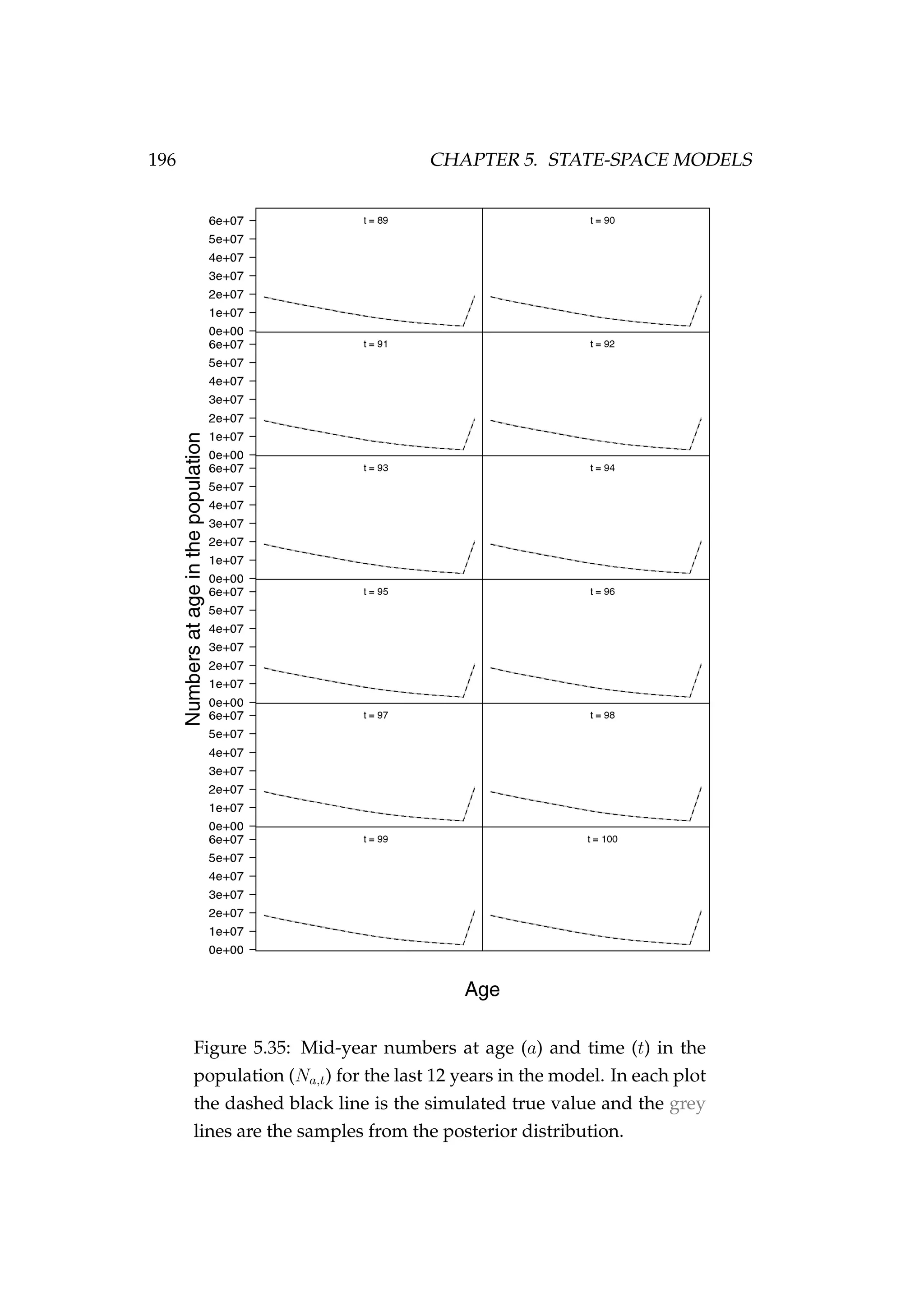
209. 5.4. AGE-STRUCTURED STATE-SPACE MODELS 197
proportions in the catch at age ((Pa)t) data very well (Figures 5.36, 5.37,
and 5.38). Finally, looking at some of the derived quantities, the poste-
Figure 5.36: Observed CPUE (It) [•] and samples from the pos-
terior distribution (qVt) [grey lines].
rior distribution of YCSs for each year of the model encompass the sim-
ulated YCSs but are not well estimated (Figure 5.39), remembering that
the recruitment variation (σ2
R) was fixed at a very low value so strong year
classes are absent from this simulated population making their estimation
difficult. The estimated Dirichlet distribution scaling (α0αt) was very well
estimated, as was the selectivity at age curve (Figure 5.30). Finally, the
estimated biomass (vulnerable, spawning stock and total) all match the
simulated biomass very well (Figure 5.30).
In this example the model appears to be able to recover the true numbers
at age latent states and key parameters reasonably well and the MCMC
performance is acceptable.

210. 198 CHAPTER 5. STATE-SPACE MODELS
Figure 5.37: Samples from the posterior distribution of the pro-
portions in the catch at age in the vulnerable portion of the
population ((Qa)t) [grey lines] and observed proportions in the
catch at age ((Pa)t) [•] for the first 12 months of the model.

211. 5.4. AGE-STRUCTURED STATE-SPACE MODELS 199
Figure 5.38: Samples from the posterior distribution of the pro-
portions in the catch at age in the vulnerable portion of the
population ((Qa)t) [grey lines] and observed proportions in the
catch at age ((Pa)t) [•] for the last 12 months of the model.

212. 200 CHAPTER 5. STATE-SPACE MODELS
Figure 5.39: Year class strengths by year (YCSt = eεp
a=1,t−σ2
R/2
)
[top left], variability of the Dirichlet distribution each year
(α0αt) [top right], selectivity at age (Sa) [bottom left] and
biomass (tonnes) by year (including the total biomass (Bt) in
green, the spawning stock biomass (SSBt) in red and the vul-
nerable biomass (Vt) in grey) [bottom right]. In each plot the
dashed black line is the simulated true value and the grey lines
are the samples from the posterior distribution.

213. 5.4. AGE-STRUCTURED STATE-SPACE MODELS 201
Model fit (releasing σ2
R)
The final test we do is to test the models performance when supplied data
simulated with more realistic recruitment variability. The final example
uses the same parameter set specified in Table 5.2 in the simulation except
for the recruitment variance parameter (σ2
R) which is changed to be σ2
R =
0.022
(rather than σ2
R = 0.0012
). Despite this increase, we are still not really
using a realistic recruitment variability value, a realistic value might be
σ2
R = 0.32
. However, as we show below, the model struggles with the
recruitment variability defined above.
Again, we leave the process error variance (σ2
p) fixed and begin by speci-
fying highly informative priors for each of the model parameters to check
for any problems in the MCMC. The recruitment variance prior is the only
change here
π(σ2
R) ∼ log N(log(0.022
), 0.05).
Unfortunately, mixing was too slow and MCMC trace plots show that the
model does not converge (Figures 5.40 and 5.41). Trace plots for the num-
bers at age latent states can be found in Appendix B.4, page 336. Many
attempts were made to improve the mixing in the MCMC given realis-
tic simulations (i.e. that used realistic recruitment variability parameters)
including MCMC runs that took over a week to complete. However, ex-
ploratory runs suggest that even if all of the key parameters are fixed,
with a high recruitment variance, adequate mixing is still not achieved in
the numbers at age and time latent states. We discuss these results further
below.

214. 202 CHAPTER 5. STATE-SPACE MODELS
Figure 5.40: MCMC trace plots [left] and posterior densities
[right] for the key model parameters. The horizontal blue lines
indicate the true parameter values as specified in the simula-
tion. All panels are made up of two separate MCMC chains of
1000 samples initialised with different random number seeds.

215. 5.4. AGE-STRUCTURED STATE-SPACE MODELS 203
Figure 5.41: MCMC trace plots [left] and density plots [right]
of the different components of the model log-likelihood includ-
ing the log-likelihood of the CPUE observations, the propor-
tions in the catch at age observations, the numbers at age latent
states, the prior contribution and the total log-likelihood. The
horizontal blue lines indicate the log-likelihood for each of the
likelihood components in the simulation given the true param-
eter values. All panels are made up of two separate MCMC
chains of 1000 samples initialised with different random num-
ber seeds.

216. 204 CHAPTER 5. STATE-SPACE MODELS
5.5 Discussion
The aim of this chapter was to introduce state-spaces models, to illustrate
how Bayesian inference performs when estimating observation and pro-
cess error simultaneously, and to develop an age-structured state-space
model that might better quantify the uncertainty in parameters of interest
within stock assessment.
Biomass dynamics models were used to introduce state-space modelling
in fisheries stock assessment. While biomass dynamics models were not
the focus of this chapter, they do provide some insight into model be-
haviour in the face of uncertainty. Estimating model parameters in sim-
ulated biomass dynamics systems is easy if uncertainty is minimal (i.e.
low observation and process error) or if informative priors are used. High
uncertainty or uninformative priors make parameter estimation more dif-
ficult. Unfortunately, the latter is the reality. Uncertainty is a defining
feature of stock assessment and rarely do we have much prior knowledge
about key parameters. However, sensible priors for key parameters can be
developed for such models. Examples illustrated in this chapter include
log-normal priors with high variance (Equations 5.11 and 5.12) or the rela-
tively informative prior developed for the magnitude of process error (σ2
p,
Equations 5.15 and 5.16).
Next, we developed an age-structured state-space model that includes
process error in the mid-year numbers at age in the population. The aim
here was to develop a more probabilistic approach to age-structured stock
assessment modelling, by replacing the standard deterministic popula-
tion dynamics equations with fully state-space formulations. This model
should better represent uncertainty in the estimates they provide. A
correctly specified model like this should also avoid the data weighting
paradigm.
It is common practice in stock assessment to assign relative weights to
different data sets (i.e. age composition data is often assigned a lower
weight relative to abundance indices). This is done so that the model fits
to abundance index data primarily, and then fits to age-composition data

217. 5.5. DISCUSSION 205
so long as the fit to these data does not result in a poor fit to the abun-
dance data. Quoting Francis (2011), if we do not assign a lower weight to
the composition data “there is a danger that any signal from abundance
data will be swamped by that from composition data, simply because the
latter data type is typically much more numerous (in terms of individual
data points”. This holds true for standard stock assessment models that
are based on deterministic population dynamics equations and often use
the multinomial distribution in fitting to composition data. However, a
properly defined probabilistic Bayesian approach should not require data
weighting because a prior distribution becomes the appropriate mecha-
nism by which we specify our prior uncertainty. For example, a prior
distribution can be used to inform the scaling parameter of the Dirichlet
distribution, which is essentially analogous to data weighting.
Estimation of model parameters and latent states in our age-structured
state-space was done using blockwise Metropolis-Hastings, avoiding the
need for maximum likelihood methods and the need to estimate a vari-
ance covariance matrix for multivariate proposals. Treating the numbers
at age and time (Na,t) for all ages and times as latent states requires thou-
sands of different MCMC proposals within a single MCMC step. The com-
putational workload here was reduced by splitting the likelihood up into
smaller components and only evaluating those components of the likeli-
hood that require evaluation during each of the MCMC proposals.
Initial exploration suggested that mixing was slow for the numbers at age
and time latent states (Na,t). To help speed up mixing, a diagonal cohort
proposal was developed (Section 5.4.1, page 177). This proposal updated
the numbers at age for each diagonal element of the Na,t matrix (cohort) in
the model by scaling the numbers at age within each cohort by a common
factor (λ∗
). The goal here was to improve mixing within cohorts by updat-
ing the entire cohort at the same time, thus increasing the acceptance rate
of proposals.
This diagonal update proposal did improve mixing substantially. How-
ever, it was not enough. When the recruitment variation (σ2
R) is low,
the model is well behaved and efficient sampling of the posterior using

218. 206 CHAPTER 5. STATE-SPACE MODELS
MCMC can be achieved. However, when σ2
R is increased (in this case to
σ2
R = 0.022
) then the MCMC fails to mix properly, even with millions of
iterations. The high correlation between the models latent states makes
efficient sampling difficult.
Future research should focus on proposals that speed up mixing for the
numbers at age and time (Na,t) latent states. For example, rather than the
diagonal cohort update that we implemented, an update based on the ex-
pected value (µa,t) could be developed. Here one might draw Na=1,t for
any selected year t, then update Na,t for years t + 1, . . . , T. The challenge
here would be deriving the correct acceptance ratio (r). Failing this, the
state-space formulation presented here requires simplification. An obvi-
ous fix would be to drop the state-space structure for some of the numbers
at age and time latent states. For example, treating Na=1,t ∀t (i.e. Y CSt as
is done in current stock assessment models, row 1) and for Na,t=1 ∀a (i.e.
non-equilibrium numbers at age in the first year, column 1) as latent states.
This is similar to what happens in current stock assessment methods.
Another area that requires further thought is around the process error
structure. Composition data that enables us to detect year classes is rarely
available in the early years of stock assessment models so there may be
little point in modelling non-equilibrium numbers at age in practice. In-
stead of using the process error matrix (σ2
a,t) defined in Equation 5.28 and
Figure 5.20, the errors could be structured in a way that allows year classes
to be semi-deterministic at the beginning of the model (e.g. Figure 5.42).
We used the programming language Julia to implement the simulation
model and MCMC sampler for this model. These types of models require
us to sample many millions of times from the posterior distribution, and
this is time consuming. Julia provides the best of both worlds with com-
putational performance approaching that of C (it is faster than C in some
cases) and a user friendly language with the ability to run interpreted code
(i.e. line-by-line as in R) or fully compiled at the command line (like C or
C++) for maximum speed. This provides the programmer the ability to
check code a single line at a time when debugging, or run as a fast MCMC
sampler/computer program.

219. 5.5. DISCUSSION 207
R0 R0 × SR(SSBt−1)
N0
a
...
N0
a
N0
A
a = 1
a = A
t = 1 t = T
σ2
p
σ2
p
σ2
p
σ2
p
σ2
p
σ2
p
σ2
p
σ2
p
σ2
p
σ2
p
σ2
p
σ2
p
σ2
p
σ2
p
σ2
p
σ2
p
σ2
p
σ2
p
σ2
p
σ2
p
σ2
p
σ2
p
σ2
p
σ2
p
σ2
p
σ2
p
σ2
p
σ2
p
σ2
p
σ2
p
σ2
p
σ2
p
σ2
p
σ2
p
σ2
p
σ2
p
σ2
p
σ2
p
σ2
p
σ2
p
σ2
p
σ2
p
σ2
p
σ2
p
σ2
p
σ2
p
σ2
p
σ2
p
σ2
p
σ2
p
σ2
p
σ2
p
σ2
p
σ2
p
σ2
p
σ2
p
σ2
R σ2
R σ2
R σ2
R σ2
R σ2
R σ2
R σ2
R
Figure 5.42: Matrix showing the direction of transitions be-
tween numbers of fish at age and time (Na,t) within the model
and the process errors variance to be used at each age a and
time t. The colours are used to highlight the 6 parts of Equa-
tion 5.21.

220. 208 CHAPTER 5. STATE-SPACE MODELS
While this is a sophisticated age-structured model, it pushes the bound-
aries of the practical limits of computing. The continual improvements be-
ing made to Julia may help speed up the model in the future, as would the
use of high performance computers. The model is already multi-threaded,
allowing multiple chains to be passed to individual computer cores to run
independently. These are then amalgamated at the conclusion of MCMC
sampling. However, the most successful speed gains are often achieved
with minor changes to the code (e.g. reparameterisation, more efficient
code). Also, MCMC can be made better with smarter proposals, an area
worthy of further research.
In summary, the major contribution provided in this chapter is the con-
struction of the posterior for an state-space age-structured model. The
future challenge is to sample from this posterior efficiently.

221. Chapter 6
Pop-up satellite archival tagging
A pop-up satellite archival tag (PSAT) is an archival tag (or data logger)
that can be attached to a fish to record data measured using sensors in
the tag. PSATs can then detach from the fish after a prespecified length of
time and are able to transmit the collected data via satellite. Alternatively,
the fish may be recaptured and the tag recovered1
. In this chapter we
discuss the development and application of a state-space model that aims
to estimate the path taken by a fish between two points (tag-release and
tag-recapture location) using data recorded by a PSAT attached to the fish.
We use Bayesian inference methods to estimate the posterior distributions
of model parameters and latent states (the position of a fish at discrete
time-steps). We use data from a PSAT deployed on an Antarctic toothfish
(Dissostichus mawsoni) in the Ross Sea as a case study (for more information
on Antarctic toothfish see Chapter 3, page 73). Lists of the variables used
throughout this chapter are given in Tables 6.1 and 6.2.
6.1 Introduction
One of the important information needs influencing the stock assessment
and management of fish stocks is understanding their movements and mi-
1
Usually a lot more data is recorded by the tag than is transmitted via satellite. If the
tag is recovered then a lot more data is available, but this is not always possible.
209

222. 210 CHAPTER 6. POP-UP SATELLITE ARCHIVAL TAGGING
Table 6.1: Description of variables, including their dimensions and units,
used throughout this chapter when discussing the process model. Equal-
area refers to the variable being in an equal-area projection (Section 6.1.3,
page 216).
Symbol Dimension Units Description
T 1 hours or weeks Number of time-steps
t 1 hours or weeks A single time-step where t =
0, . . . , T
xt 2 m Equal-area projected position of a
fish at time t, xt = (xt, yt) (Equa-
tion 6.5)
x0 2 m Start position (equal-area), x0 = xt=0
(Equation 6.5)
xT 2 m End position (equal-area), xT = xt=T
(Equation 6.5)
σx 1 m Standard deviation of the hourly or
weekly horizontal movement of a
fish (Equation 6.5)
φ 1 degrees Latitude (Equation 6.1)
λ 1 degrees Longitude (Equation 6.1)
φ0 1 degrees Projection centre (latitude, Equa-
tion 6.1)
λ0 1 degrees Projection origin (longitude, Equa-
tion 6.1)
R 1 m Radius of the Earth (e.g. R =
6378137m at the South Pole, Equa-
tion 6.3)

223. 6.1. INTRODUCTION 211
Table 6.2: Description of variables, including their dimensions and units,
used throughout this chapter when discussing the observation models.
Symbol Dimension Units Description
at T g Fish acceleration at time t (1g =
9.8ms−1)
bt T nT Magnetic field strength at time t
ct T ◦C Sea temperature at time t (Equa-
tions 6.7, 6.8, and 6.9)
dt T m Fish depth at time t (Equa-
tions 6.10, 6.11, and 6.12)
mt T months Month at time t
µc
x,d,m 31 × 121 × 79 × 12 ◦C Temperature covariate layer (latitude
× longitude × depth × month, Equa-
tions 6.7 and 6.9)
σc
x,d 31 × 121 × 79 ◦C Standard deviation of temperature
covariate layer (latitude × longitude
× depth, Equations 6.7 and 6.9)
σc 1 ◦C Standard deviation of temperature
when assumed constant with lo-
cation and depth (Equations 6.8
and 6.9)
µd
x 1001 × 5001 m Depth covariate layer (latitude × lon-
gitude, Equations 6.10 and 6.11)
σd 2 m Split-normal standard deviation of
depth (Equation 6.11)

224. 212 CHAPTER 6. POP-UP SATELLITE ARCHIVAL TAGGING
grations. Modelling the movements of fish populations requires estimates
of the routes, timing, and duration of movements, not simply demonstrat-
ing a link between geographical regions. This includes information on fish
that may migrate to previously unfished or closed areas (e.g. areas closed
as marine protected areas). Other types of movement information, such
as patterns in vertical movements, are also becoming important in stock
assessment and in understanding the ecosystem role of different species,
as their depth distribution affects which species they interact with, both as
predators and as prey (Horodysky et al. 2007).
Both horizontal and vertical movement information about individuals can
be gathered through the use of PSATs (Godo & Michalsen 2000, Williams
& Lamb 2002, Seitz et al. 2005, Brown et al. 2011). Most positioning stud-
ies using archival tag data rely on light-based geolocation methods, some-
times with the addition of sea surface temperature data to improve esti-
mates of location (Welch & Eveson 1999, Teo et al. 2004, Neilsen et al. 2006).
The variables recorded by modern PSATs include (but are not limited to)
acceleration, depth, light, magnetic field strength and temperature.
Hanchet et al. (2008) interpreted existing fishery and biological data to
hypothesise that adult Antarctic toothfish (in the Ross Sea) move from the
continental slope region to northern seamounts to spawn, and then return
to the slope to feed and regain condition. However, the actual degree of
connectivity, range of spawning destinations, level of return migration,
and duration of migrations remains uncertain (Parker, Hanchet & Horn
2014). Furthermore, toothfish inhabit deep waters under ice and below the
photic zone and long periods of constant daylight or constant darkness
preclude the use of light for Antarctic toothfish geolocation year round.
Despite these challenges, we suspect that the sensors in PSATs may be
able to provide other information that might prove useful in geolocating
Antarctic toothfish.
In January 2013, four PSATs were attached to toothfish and released in the
Ross Sea (Table 6.3, Figure 6.1). The four fish chosen were large and in
excellent condition (Parker, Webber & Arnold 2014). Despite being pro-
grammed to pop-up after one year and transmit data via satellite, none of

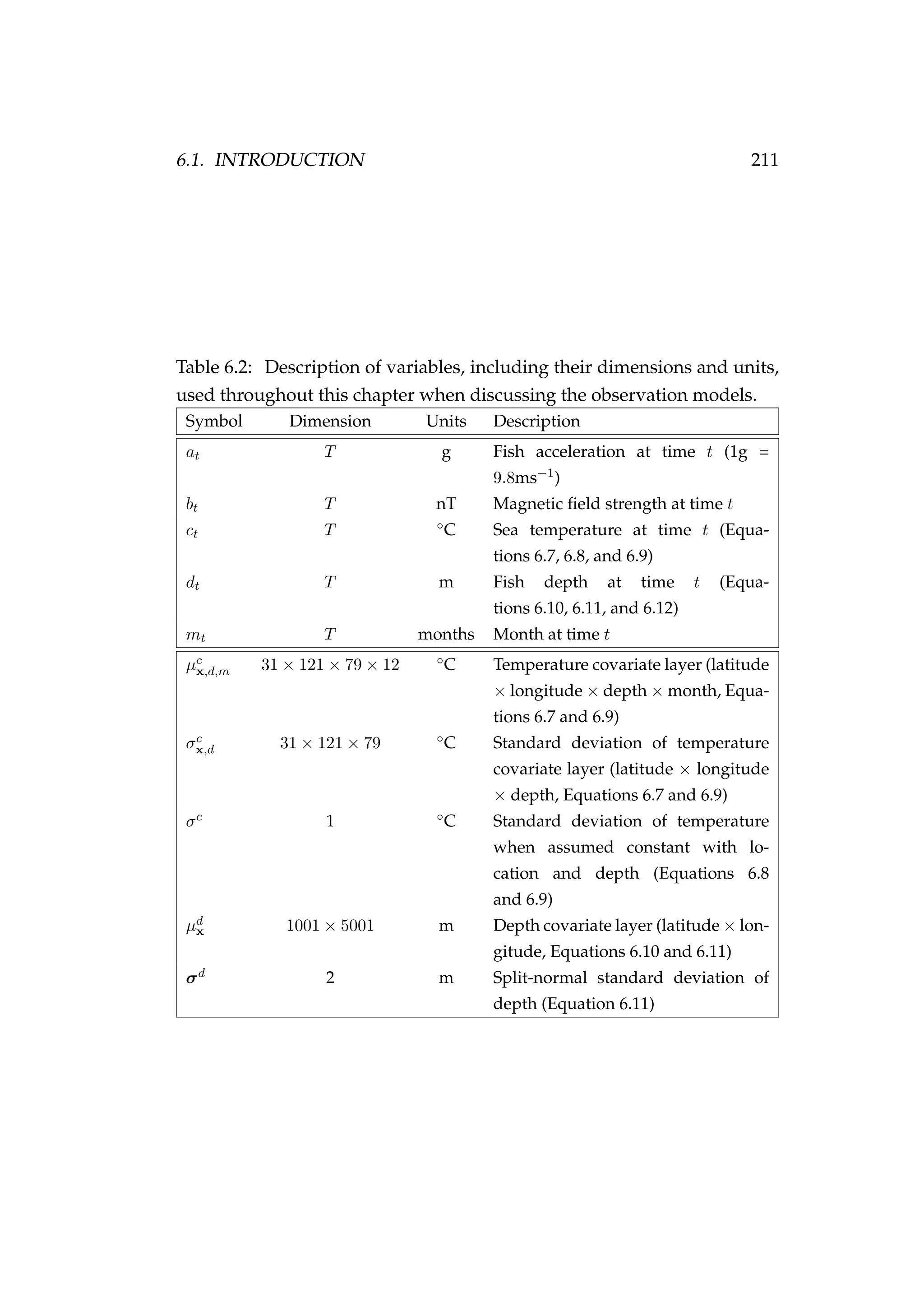
225. 6.1. INTRODUCTION 213
Table 6.3: Details of four pop-up satellite archival tag (PSAT) releases on
Antarctic toothfish (Dissostichus mawsoni) in the Ross Sea during January
2013. Columns include a unique tag identification number for each tagged
fish, the date of capture/release, the length of each fish, their weight, the
depth of water that the fish were caught in, and the latitude and longitude
of their capture/release.
Tag ID Date Length Weight Depth Latitude Longitude
(dd-mm-yyyy) (cm) (kg) caught (m)
206 22-01-2013 167 51.2 1058 -71.72 176.97
121 22-01-2013 150 39.0 1006 -71.70 176.97
162 23-01-2013 150 39.0 838 -71.80 177.11
179 23-01-2013 160 47.5 914 -71.80 177.17
Figure 6.1: A toothfish being tagged with a pop-up satellite
archival tag (PSAT) [left] and a PSAT [right] (photo credit S.
Parker, NIWA).

226. 214 CHAPTER 6. POP-UP SATELLITE ARCHIVAL TAGGING
the tags popped off and transmitted. However, one of these fish was re-
captured prior to its programmed pop-off date the following fishing sea-
son on 24 December 2013, 335 days later (tag 121, Figure 6.2). In addition,
a fifth tag (tag 186) was deployed as a towed body at a depth ranging be-
tween about 8m depth and the surface, approximately 100m behind the
vessel on a transect from the southern Ross Sea to a latitude of about 60◦
S
(Figure 6.2). A series of global positioning system (GPS) recordings were
taken along this transect (Appendix C.1, page 342).
Our aim is to develop a state-space model that can estimate the path
taken by a fish between tag-release and tag-recapture location using data
recorded by PSATs.
6.1.1 Variables recorded by the tags
Variables recorded by the deployed PSATs included date and time, accel-
eration in three dimensions (3D), depth with a resolution of 15m, light,
magnetic field strength in 3D with a resolution of approximately 15 nano
Teslas (nT), and temperature with a resolution of 0.002◦
C. Acceleration
and magnetic field strength were measured along three orthogonal axes
(x, y, z). These correspond to the 3D components of acceleration and the
northerly, easterly and vertical components of the Earths magnetic field,
respectively. Tag 121 was programmed to record all variables every 10
minutes. Tag 186 recorded every 16 seconds.
6.1.2 Environmental data or models (covariates)
The PSAT data can be compared with values of the same variables from
measured data sets or global or regional models. Depth (m) observed by
the tag dt at time t can be compared to a bathymetric map of the Ross Sea
region (Figure 6.2, Davey 2004). These data are available in cells measur-
ing 0.01◦
latitude by 0.01◦
longitude from -79◦
to -69◦
latitude and 160◦
to
210◦
longitude (a 1001 × 5001 matrix of latitude by longitude). We refer
to these data the depth covariate layer µd
x where the subscript x indexes

227. 6.1. INTRODUCTION 215
Figure 6.2: Expected depth (m) throughout the Ross Sea re-
gion (Davey 2004). The tag-release [•] and recapture [•] loca-
tions of the tagged fish (tag 121) are shown, as are the recorded
GPS coordinates associated with the towed tag (tag 186) [•].
Regions in grey represent land. The aspect ratio has been cho-
sen so that the plot is approximately equal area projected.
the 2D horizontal location. Any depth below the surface (0m) is given
as a negative value (e.g. the depth at (-75.562, 180.021) is -565.0m). Any-
thing above the surface is given a positive value (these depths are actually
heights, e.g. the “depth” at (-75.562, 160.021) is 1149.5m which is on land).
Expected temperature (◦
C) and the standard deviation of temperature (◦
C)
are available from the Commonwealth Scientific and Industrial Research
Organisation (CSIRO) Atlas of Regional Seas (CARS) 2009 model (Fig-
ures 6.3 and 6.4, Ridgeway et al. 2002, www.cmar.csiro.au/cars). This
model provides estimates of temperature by latitude, longitude, depth
and month. These model outputs are available in cells measuring 0.5◦
lat-
itude by 0.5◦
longitude across a variable bin size for depth (ranging from
0 to 5631m). The spatial range of these data extends from -75◦
to -60◦
lati-
tude and 150◦
to 210◦
longitude (a 121 × 31 × 79 × 12 array of latitude by
longitude by depth by month). The standard deviation of temperature in
each cell is provided by longitude, latitude and depth (a 31×121×79 array
of latitude by longitude by depth). We refer to these model outputs as the
temperature covariate layer µx,d,m and the standard deviation of temper-
ature covariate layer σx,d where the subscript x indexes the 2D horizontal
location, d the depth, and m the month. The temperature can be nega-
tive or positive. Some of the values in the array are NaN (not a number),

228. 216 CHAPTER 6. POP-UP SATELLITE ARCHIVAL TAGGING
these refer to latitude/longitude/depth/month combinations that are on
land or below the sea floor. The standard deviation of temperature values
are all positive besides the values in the array are NaN. We note that the
CARS model does not represent estimates of the temperature at the time
of tagging. Instead, CARS is a digital climatology, representing the aver-
age monthly conditions over the period of modern ocean measurement,
and average seasonal cycles for that period. It is derived from all available
historical subsurface ocean property measurements - primarily research
vessel instrument profiles and autonomous profiling buoys. This is an im-
portant limitation on its utility in inferring fish movements, particularly
on small spatial scales.
6.1.3 Projection
The start and end locations of the PSATs were recorded in latitude and
longitude (WGS84), as were the data on depth and temperature described
above. However, the process model (described below in Section 6.2.1,
page 220) must operate in equal-area projection. This is because the fish’s
movement on a 2D horizontal plane is assumed to follow a bivariate nor-
mal distribution with a constant variance in physical distance (rather than
in latitude/longitude).
The spherical Lambert azimuthal equal-area projection is a mapping from
a sphere to a disk (Snyder 1926). It accurately represents area in all re-
gions of the sphere (but it does not accurately represent angles, Figure 6.5).
Given the parameters R, φ0, λ0, φ and λ we can use the transformation
equations
x = Rk cos φ sin (λ − λ0) ,
y = Rk (cos φ0 sin φ − sin φ0 cos φ cos (λ − λ0)) , (6.1)
where (x, y) are the equal-area projected latitude and longitude (m), (φ, λ)
are the latitude and longitude (WGS84, in radians) to be converted, (φ0, λ0)
are the latitude and longitude of the projection center and origin (in radi-

229. 6.1. INTRODUCTION 217
Figure 6.3: Expected temperature (◦
C) at approximately 0, -50,
-100, -500, -1000 and -1500m depth during February. The tag-
release [•] and recapture [•] locations of the tagged fish (tag
121) are shown, as are the recorded GPS coordinates associated
with the towed tag (tag 186) [•]. Regions in grey represent land
or the sea floor. The aspect ratio has been chosen so that the
plot is approximately equal area projected.

230. 218 CHAPTER 6. POP-UP SATELLITE ARCHIVAL TAGGING
Figure 6.4: Expected standard deviation of temperature (◦
C) at
approximately 0, -50, -100, -500, -1000 and -1500m depth. The
tag-release [•] and recapture [•] locations of the tagged fish (tag
121) are shown, as are the recorded GPS coordinates associated
with the towed tag (tag 186) [•]. Regions in grey represent land
or the sea floor. The aspect ratio has been chosen so that the
plot is approximately equal area projected.

231. 6.1. INTRODUCTION 219
Figure 6.5: A series of points plotted in latitude and longi-
tude [left] and the same points converted to Lambert azimuthal
equal-area projection in km [right].
ans), R is the radius of the earth (m, Equation 6.3), and
k =
2
1 + sin φ0 sin φ + cos φ0 cos φ cos (λ − λ0)
.
The inverse formulas are
φ = sin−1
cos c sin φ0 +
y sin c cos φ0
ρ
,
λ = λ0 + tan−1 x sin c
ρ cos φ0 cos c − y sin φ0 sin c
, (6.2)
where
ρ = x2 + y2 and c = 2 sin−1 1
2
ρ .
These equations allow us to transform any estimated location of a fish
from equal-area projection xt (in the process equation of the state-space
model) to latitude and longitude (the Bathymetric and temperature data
are in this form), or vice versa. We set φ0 = −70◦
and λ0 = 175◦
so that our
projection centre and origin are close to the tagged fish and the towed tag
to give an accurate projection.

232. 220 CHAPTER 6. POP-UP SATELLITE ARCHIVAL TAGGING
The geocentric radius of the Earth R (distance from the Earth’s center to a
point on the spheroid) given the geodetic latitude φ is
R =
(a2 cos φ)2
+ (b2 sin φ)2
(a cos φ)2
+ (b sin φ)2 , (6.3)
where a is the equatorial radius (6378.1370km) and b is the polar radius
(6356.7523km). Given φ0 = −70◦
we calculate R = 6359272.44m.
6.2 Model development
State-space models (SSMs) can be used to estimate the latent state of un-
observable processes from observed data sets. There are two main com-
ponents to any SSM: the process model which describes how the states
evolve in time, and the observation model(s) that describe how the states
are linked to observations. Here the latent states are the geographical lo-
cations of the fish between release and recapture (equal-area projected lat-
itude and longitude). The observed data set includes measures of depth,
temperature, light, magnetic field strength and acceleration collected at
regular intervals by the tag.
The model is written in Julia (http://julialang.org/), a high-level,
high-performance dynamic programming language for technical comput-
ing. Unlike languages such as R, Julia code is compiled before execution,
which is the main reason for its superior speed. Moreover, Julia makes
parallel computing easy, therefore our MCMC algorithm is multi-threaded
which greatly reduces computational time. The model is written so that
different components of the model can be turned on and off easily. This
allows us to turn off or modify the prior, process model, or any of the
observation models independently.
6.2.1 The process model
The process model describes how an individual fish moves through con-
tinuous space (equal-area horizontal) and discrete time. It does not model

233. 6.2. MODEL DEVELOPMENT 221
the vertical dynamics of the fish as the depth is recorded by the tag (and
assumed to be known without error). The parameters of the model are
the standard deviation of the fish’s horizontal movement σx (m) and the
discrete hidden location latent states x1, . . . , xT−1 (an equal-area projected
latitude/longitude pair at each time-step t with units m). The start lo-
cation (x0) and the end location (xT ) are assumed to be known without
error (i.e. these points are fixed). These points and all latent states (xt)
are defined as the distance (m) from the specified reference point (φ0, λ0),
schematically:
xt
x0 xT (φ0, λ0)
For simplicity, we begin by describing the model in one dimensional (1D)
space. The notation is changed to two dimensional (2D) space later. In 1D,
the full probability of a path {xt}T
t=0 is
P(x0, ..., xT ) = P(xT |xT−1) × · · · × P(x1|x0)P(x0).
The probability of a path conditional on the start point (x0) and the end
point (xT ) is
P(x1, ..., xT−1|x0, xT ) =
P(x0, · · · , xT )
P(x0, xT )
=
P(x0, · · · , xT )
P(xT |x0)P(x0)
=
1
P(xT |x0)
P(xT |xT−1) × · · · × P(x1|x0)
∝ P(xT |xT−1) × · · · × P(x1|x0)
where the proportionality neglects any terms not explicitly dependent on
x1, . . . , xT−1. The probability of any point along a path (xt) conditional on
the previous point (xt−1) and the next point (xt+1) is
P(xt|xt−1, xt+1) =
P(xt−1, xt, xt+1)
P(xt−1, xt+1)
=
P(xt+1|xt)P(xt|xt−1)P(xt−1)
P(xt−1, xt+1)
∝ P(xt+1|xt)P(xt|xt−1).

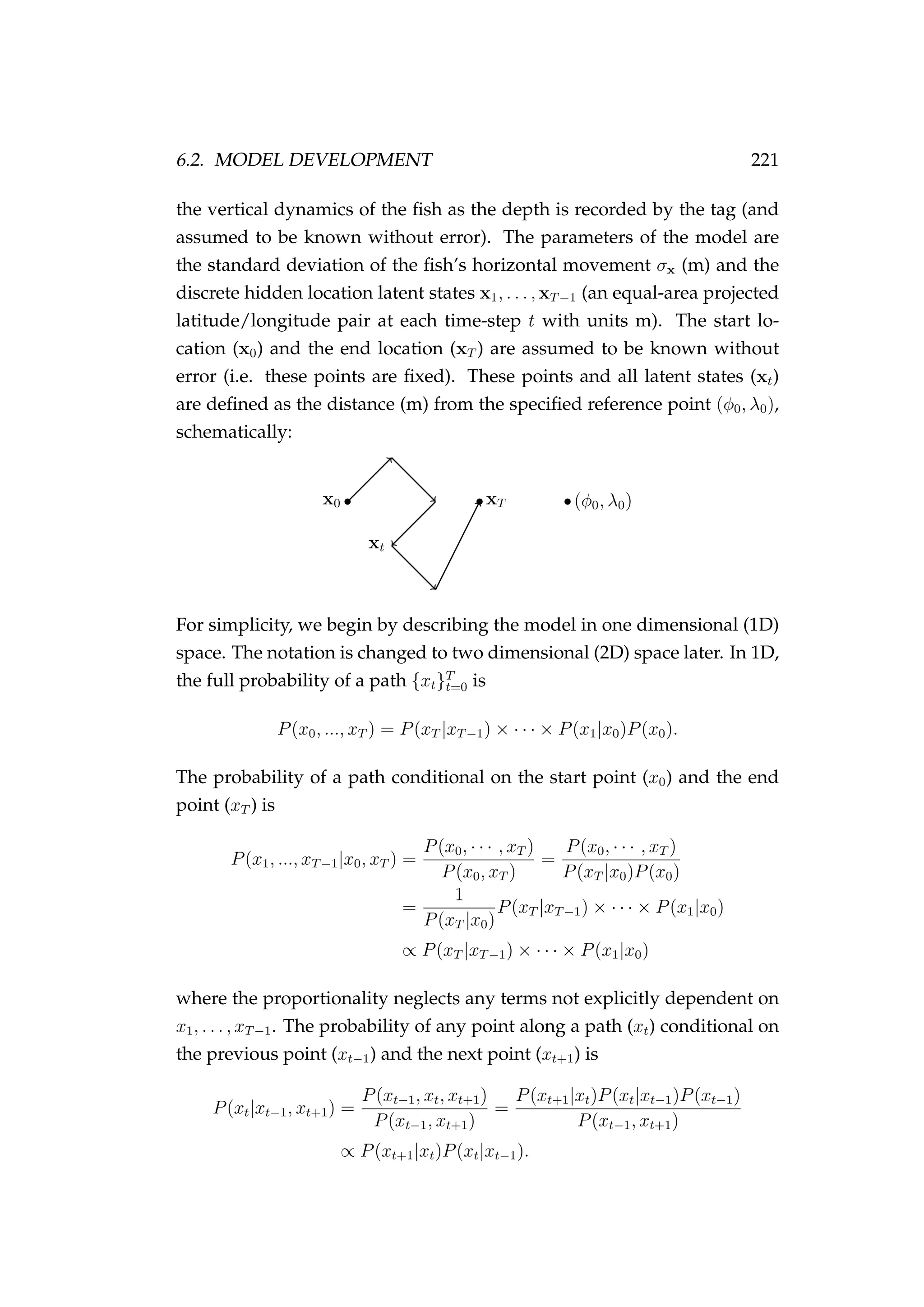
234. 222 CHAPTER 6. POP-UP SATELLITE ARCHIVAL TAGGING
Assuming a normally distributed random walk with standard deviation
σx we write
xt|xt−1, σx ∼ N xt−1, σ2
x .
Conditional on both the previous point (xt−1) and the next point (xt+1) this
becomes
P(xt|xt−1, xt+1, σx) ∝ 2πσ2
x
−1
2
exp −
1
2σ2
x
(xt+1 − xt)2
× 2πσ2
x
−1
2
exp −
1
2σ2
x
(xt − xt−1)2
∝ exp −
1
2σ2
x
2x2
t − 2xtxt+1 − 2xtxt−1
∝ exp −
1
2σ2
x
2 x2
t − 2xt
xt+1 + xt−1
2
∝ exp

−
1
2 σ2
x
2
xt −
xt+1 + xt−1
2
2


xt|xt−1, xt+1, σx ∼ N
1
2
(xt−1 + xt+1),
σ2
x
2
.
In 2D this simply becomes
xt|xt−1, σx ∼ N xt−1, σ2
xI , (6.4)
xt|xt−1, xt+1, σx ∼ N
1
2
(xt−1 + xt+1) ,
σ2
x
2
I , (6.5)
where I is a 2 × 2 identity matrix. We can generalise this further for any
point xj to any other point xk
xt|xt−j, xt+k, σx ∼ N
1
j + k
(kxt−j + jxt+k) ,
jkσ2
x
j + k
I .
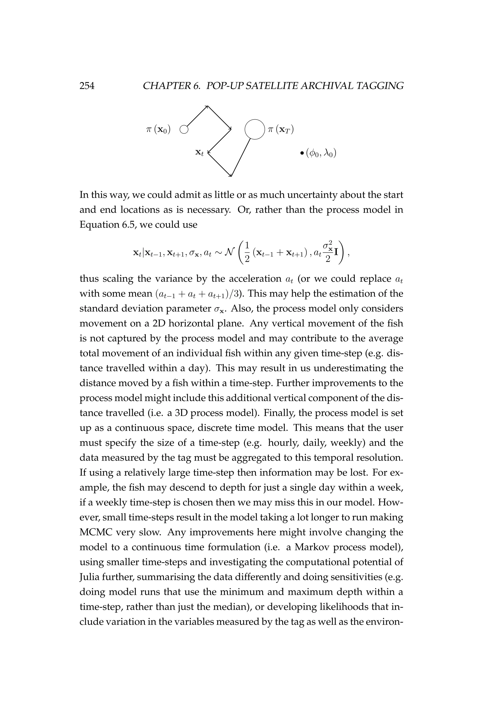
Conditional only on x0 and xT we can sample from Equation 6.5 using a
Gibbs sampler. The expected path of xt is a straight line
E[xt|x0, xT ] = x0 +
t
T
(xT − x0) . (6.6)
Unlike horizontal movement, we place no constraint on the vertical move-
ment of the fish (i.e. dt is assumed to be independent of dt−1).

235. 6.2. MODEL DEVELOPMENT 223
Figure 6.6: Observations recorded by the towed tag (tag 186)
every 16 seconds [grey] and hourly median [red] from 23
February 2012 to 26 February 2012.

236. 224 CHAPTER 6. POP-UP SATELLITE ARCHIVAL TAGGING
Figure 6.7: Observations recorded by the tagged fish (tag 121)
every 10 minutes [grey] and daily median [red].

237. 6.2. MODEL DEVELOPMENT 225
6.2.2 Observation models
Data for the towed tag (tag 186) and the tagged fish (tag 121) are shown
in Figures 6.6 and 6.7. Observation models were developed to model the
recorded variables depth and temperature. Although acceleration, light,
and magnetic field strength were recorded by the tag, they are not used
here.
Light has been used successfully in the past to help estimate a fish’s lo-
cation through time (Welch & Eveson 1999). However, toothfish inhabit
deep waters under ice and below the photic zone. In addition, long peri-
ods of constant daylight or constant darkness preclude the use of light for
Antarctic toothfish geolocation year round.
Models are available that describe the total magnetic field strength both
spatially and temporally. However, preliminary exploration of the data
suggested that the variability in the magnetic field strength recorded by
the tags drowned out any pattern in these data across their spatial range
(Figures 6.6 and 6.7). We simply plot the magnitude of total magnetic field
strength.
We do not attempt to model acceleration in this project. However, we
do provide some ideas for future research in the discussion (Section 6.7,
page 253) and plot the magnitude of acceleration.
Temperature
The temperature observation model links the temperature observed by the
tag ct to the temperature covariate layer µc
x,d,m and the standard deviation
of temperature covariate layer σc
x,d (or the fixed standard deviation of tem-
perature σc
if this is being used). This model consists of a lookup function
coupled with a likelihood function.
The lookup function is written to access the temperature and standard
deviation of temperature arrays given a latitude, longitude, depth and
month. If the given latitude and/or longitude exceeds the bounds of the
temperature layer, then the function returns the value NaN (not a num-

238. 226 CHAPTER 6. POP-UP SATELLITE ARCHIVAL TAGGING
ber). Otherwise it returns the temperature at that location and month
along with the standard deviation of temperature in that location. The
returned values could be NaN (see Section 6.1.2, page 216).
The temperature given the horizontal location of the tag xt (latitude and
longitude), depth (m) of the tag dt, and the month mt at time t = 1, . . . , T −
1 is is assumed to be
ct|xt, dt, mt, µc
x,d,m, σc
x,d ∼ N µc
xt,dt,mt
, σc
xt,dt
2
(6.7)
or
ct|xt, dt, mt, µc
x,d,m, σc
∼ N µc
xt,dt,mt
, (σc
)2
(6.8)
depending on whether or not the spatially varying standard deviation of
temperature covariate layer σc
x,d is to be used or not (the alternative being
a fixed standard deviation σc
). The log-likelihood function of the temper-
ature is
ct|xt, dt, mt, µc
x,d,m, σc
x,d =



−∞ if µc
xt,dt,mt
= NaN
− log σc
xt,dt
−
(ct−µc
xt,dt,mt
)
2
2(σc
xt,dt
)
2 otherwise
.
(6.9)
If the lookup function returns NaN, then the log-likelihood evaluates to
−∞ (i.e. the path is limited to the range of the temperature data).
Depth
A lookup function is written to access the depth covariate layer matrix
(Section 6.1.2, page215) given a latitude and longitude. If the given loca-
tion exceeds the bounds of the depth layer, then the function returns NaN
(not a number). Otherwise it returns the depth at that location (even if the
depth is > 0).
The depth data may be used in two ways: using depth to simply exclude
certain areas of 2D space (by identifying land as inaccessible to the fish),
or by assuming that the fish follows the sea floor and developing a distri-
bution to describe the fish’s behaviour with respect to the sea floor.

239. 6.2. MODEL DEVELOPMENT 227
We use the first option to model the towed tag (tag 186, Section 6.4,
page 233) and in a simulation study (Section 6.5, page 240). If using this
option the log-likelihood function of the depth is
dt|xt, µd
x =



−∞ if dt < µd
xt
0 otherwise
. (6.10)
The choice of a constant log-likelihood of 0 here is arbitrary and any con-
stant value could be used. This function stops the model from explor-
ing space where there is land or where the sea floor is shallower than the
depth of the fish. It does not stop the model from exploring space beyond
the boundaries of the data (i.e. when the lookup function returns NaN).
Also, unlike horizontal movement, we place no constraints on the vertical
position of the fish relative to the sea floor. To explain, we use Figure 6.8
below. Let us assume that each of the red points in the figure represent the
Figure 6.8: An example diagram of the sea floor, sea surface
(0m), and the range of some depth data (e.g. µd
x). Proposed
locations for model exploration are shown using the [•] points
a, b, c and d.
proposed location of our fish within a time-step in our MCMC. Point a is
within the range of the depth covariate layer, but the proposed location is
on land (actually underground, dt < µd
x). In this case, the log-likelihood

240. 228 CHAPTER 6. POP-UP SATELLITE ARCHIVAL TAGGING
would evaluate to −∞ and the move would be rejected. Point b is within
the range of the depth covariate layer, and above the sea floor (dt ≥ µd
x),
therefore the log-likelihood evaluates to 0 and the proposed move could
be accepted. Point c is within the range of the depth covariate layer, but
the proposed location is deeper than the expected depth in this location
(dt < µd
x). In this case, the log-likelihood would evaluate to −∞ and the
move would be rejected. Finally, point d exceeds the range of the depth
covariate layer. In this case, we don’t know if the proposed point is above
or below the sea floor or over land. Here we assume that the move is
acceptable and set the log-likelihood to 0 (but see Section 6.2.3, page 229
below).
When modelling the tagged fish (tag 121) we used a split-normal distribu-
tion to link the known depth (m) of the fish to the depth throughout the
Ross Sea (Figure 6.9). In the first instance, we assume the fish will gener-
Figure 6.9: The assumed prior of the distribution of tagged fish
(tag 121) recorded depth relative to bathymetric data (shown
for example at 500m with σ1 = 50m and σ2 = 5m).

241. 6.2. MODEL DEVELOPMENT 229
ally follow the sea floor. The split-normal also provides some probability
density a short distance below the sea floor to account for any uncertainty
in the measured depth throughout the region. In this way, we are using
the split-normal distribution to “stick” the fish to the sea floor, but allow
the fish to go little deeper than the bathymetric data suggests the depth is,
and allow the fish to explore space above the sea floor as well. We com-
pare the median depth observed by the tag dt during time t to the depth
expected in that location
dt|xt, µd
x, σd
∼ SN µd
x, (σd
)2
, (6.11)
where σd
= {σd
1, σd
2}. The log-likelihood function for depth is
dt|xt, µd
x, σd
= log SN µd
x, (σd
)2
. (6.12)
The split-normal distribution will only be an appropriate choice for species
that tend to follow the sea-floor. If modelling pelagic species then the
method that excludes areas would be a better choice (Equation 6.10).
The split-normal distribution is formed by merging two normal dis-
tributions about a common mode. The probability density function
(PDF) of a split-normal distribution is given by
f(x; µ, σ1, σ2) =



A exp −(x−µ)2
2σ2
1
if x < µ
A exp −(x−µ)2
2σ2
2
otherwise,
where
A =
2
π
(σ1 + σ2)−1
.
The component distributions of the split-normal distribution can have
two different variances. To ensure that the resulting PDF integrates to
1, the normalising constant A is used.
6.2.3 Additional considerations
To stop the fish from exceeding the bounds of any, or both, covariate layers
we can use uniform priors. These priors could be applied to the equal-area

242. 230 CHAPTER 6. POP-UP SATELLITE ARCHIVAL TAGGING
projected proposals (x, y) or the proposals in latitude and longitude (φ, λ).
For example, if we wanted to restrict the path to being within the range of
the temperature covariate layer we would use
π(φ) ∼ U(−75, −60),
π(λ) ∼ U(150, 210)
noting that this is not uniform in (x, y).
In summary, we make the following modelling assumptions:
• all data measured by the tag (at, bt, ct, dt, mt) are measured without
error
• the start location (x0) and end location (xT ) are fixed and known
without error
• the standard deviation parameter σx is constant over time t
• the fish does not leave the bounds of the temperature covariate layer
in the towed tag (tag 186) and simulation models
• the fish does not leave the bounds of the depth or temperature co-
variate layers in the tagged fish (tag 121) model
• if using the split-normal distribution when modelling depth, the pa-
rameter σd
is assumed known and is σd
= {50, 5}
• if using a constant (with location and depth) standard deviation of
temperature, the value is fixed at σc
= 0.1◦
C
The assumed parameters of the split-normal distribution (σd
= {50, 5})
were chosen as they represent reasonable guesses at how far above the sea
floor a toothfish might venture (i.e. standard deviation of 50m) and how
uncertain our bathymetric data are (standard deviation of 5m).
6.3 Bayesian inference
We are interested in the probabilistic relationship between the following:

243. 6.3. BAYESIAN INFERENCE 231
• The data: the median observed temperature (ct) and median ob-
served depth (dt) during time t. Let y = {ct, dt}T−1
t=1
• The covariates: the month (mt) during time t, the expected temper-
ature (µc
x,d,m) in location x, at depth d during month m, the standard
deviation of temperature (σc
x,d) in location x at depth d, and the ex-
pected depth (µd
x) in location x. Let z = {{mt}T−1
t=1 , µc
x,d,m, σc
x,d, µd
x}
• The unknown nuisance parameter: the standard deviation of hori-
zontal movement (σx)
• The known parameters: the start (x0) and end (xT ) locations and
the and the split-normal standard deviation of depth (σd
). Let ω =
{x0, xT , σd
} (and possibly also σc
)
• The unknown latent states: the horizontal location of the fish (xt) at
time t. Let x = {xt}T−1
t=1
Using Bayes theorem, the posterior distribution of the model parameters
(φ) and the latent states (x), given the data (y), covariates (z) and known
parameters (ω) is
π(σx, x|y, z, ω) ∝ π(σx)π(x|ω, σx)π(y|x, z, ω), (6.13)
where for any t
π(x|ω, σx) = π(xt|xt−1, xt+1, σx) see Equation 6.5,
π(y|x, z, ω) = π(y|x, z, σd
)
=
T−1
t=1
π(ct, dt|xt, dt, mt, µc
x,d,m, σc
x,d, µd
x, σd
)
=
T−1
t=1
π(ct|xt, dt, mt, µc
x,d,m, σc
x,d) ×
T−1
t=1
π(dt|xt, µd
x, σd
)
see Equations 6.7 and 6.11.

244. 232 CHAPTER 6. POP-UP SATELLITE ARCHIVAL TAGGING
6.3.1 Blockwise Metropolis-Hastings algorithm
Posterior distributions of the model parameters and states are estimated
using MCMC. We draw samples from the joint posterior distribution using
a blockwise Metropolis-Hastings algorithm with a log-normal proposal
for the model’s parameter (σx) and bivariate normal proposals for the la-
tent states ({xt}T−1
t=1 , see Appendix A.3, page 325, for a description of a gen-
eralised sampler). We begin by initialising σ
(0)
x ∼ π (σx) and x
(0)
t (simply
a straight line between x0 and xT , see Equation 6.6). We specify the stan-
dard deviation of the proposal distribution σq, and then begin sampling
for i = 1, 2, ...
1. Propose σ∗
x ∼ qσ σ
(i)
x |σ
(i−1)
x . Here we draw log (σ∗
x) ∼
N log σ
(i−1)
x , σ2
q .
2. Compute the acceptance probability rσ (see Equation 6.14).
3. Draw u ∼ U(0, 1).
4. Accept σ∗
x if u < rσ and set σ
(i)
x ← σ∗
x, otherwise reject σ∗
x and set
σ
(i)
x ← σ
(i−1)
x .
5. For t = 2, ..., T − 1
(a) Propose x∗
t ∼ qx x
(i)
t |x
(i−1)
t−1 , x
(i−1)
t+1 , σ
(i)
x .
Here we draw a new proposal from a multivariate normal
x∗
t |x
(i−1)
t−1 , x
(i−1)
t+1 , σ
(i)
x ∼ N 1
2
x
(i−1)
t−1 + x
(i−1)
t+1 ,
σ
(i)
x
2
2
I .
(b) Compute the acceptance probability rx (see Equation 6.15).
(c) Draw u ∼ U(0, 1).
(d) Accept x∗
t if u < rx and set x
(i)
t ← x∗
t , otherwise reject x∗
t and set
x
(i)
t ← x
(i−1)
t .

245. 6.4. TAG 186: THE TOWED TAG 233
The acceptance probabilities (rσ and rx) are defined as
rσ = min

1,
π (x|ω, σ∗
x)
π x|ω, σ
(i−1)
x
×
π (σ∗
x)
π σ
(i−1)
x
×
qσ σ
(i−1)
x |σ∗
x
qσ σ∗
x|σ
(i−1)
x


= min

1,
π (x|ω, σ∗
x)
π x|ω, σ
(i−1)
x
×
π (σ∗
x)
π σ
(i−1)
x
×
σ∗
x
σ
(i−1)
x

 , (6.14)
and
rx = min

1,
π (yt|x∗
t , z, ω)
π yt|x
(i−1)
t , z, ω
×
π x∗
t |x
(i−1)
t−1 , x
(i−1)
t+1 , ω, σ
(i)
x
π x
(i−1)
t |x
(i)
t−1, x
(i)
t+1, ω, σ
(i)
x
×
qx x
(i−1)
t |x∗
t−1, x∗
t+1, σ
(i)
x
qx x∗
t |x
(i−1)
t−1 , x
(i−1)
t+1 , σ
(i)
x

 . (6.15)
The calculation of rσ requires the evaluation of the likelihood along the
whole path (for t = 1, . . . , T − 1). The calculation of rx only requires eval-
uation of the likelihood for a single location (i.e. a time-step t).
All MCMC simulations consisted of a burn-in of 55000 iterations, followed
by 1 million iterations with a thinning rate of 500 resulting in a sample of
2000. Parallel tempering was used as the depth and temperature likeli-
hood surfaces are very complex and multi-modal (imagine the bottom of
the sea floor as a likelihood surface). Three different tempered chains were
used throughout (β = {1.0, 0.9, 0.8}, see Chapter 2, page 68 for an expla-
nation of parallel tempering).
6.4 Tag 186: the towed tag
Tag 186 was deployed as a towed body approximately 100m behind a ves-
sel on a transect though the Ross Sea (Figure 6.10). While being towed the
tag recorded environmental variables every 16 seconds (Figure 6.6). These
data show that the tag was between 8m depth and the surface along the
transect. There is a clear pattern in the light level throughout each day.
As the tag is towed north the temperature gradually increases from below

246. 234 CHAPTER 6. POP-UP SATELLITE ARCHIVAL TAGGING
Figure 6.10: The temperature (◦
C) [top] and standard deviation
of temperature [bottom] at approximately 5m depth. The black
points [•] indicate the series of recorded GPS coordinates asso-
ciated with the towed tag (tag 186). Also shown are the start
[•] and end [•] location of tag 121. Regions in grey represent
land. The plot region is adjusted to be approximately equal
area projected.

247. 6.4. TAG 186: THE TOWED TAG 235
zero to about 4◦
C. There is little pattern and high variation in both the total
magnetic field strength and acceleration of the tag along the transect.
GPS coordinates were recorded along this transect. Several of the GPS
points that appear to be outliers were removed along with those points
that were outside the range of the CARS temperature data set leaving
72 GPS coordinates (Figure 6.10, Appendix C.1, page 341). The start lo-
cation was x0 = (−72.770833, 174.436667) and the end location was at
xT = (−61.550000, 176.301944). At each of the GPS locations the tem-
perature recorded by the tag was identified and compared with the tem-
perature expected by the CARS model at each of the GPS locations. The
temperature expected by the CARS model showed the same general in-
creasing trend as the temperature observed by the tag over the four day
period, however the temperature observed by the tag was often higher
than that expected by the model, particularly on Friday (23 February 2012,
Figure 6.11).
We fit the model to the tag 186 temperature data to estimate the horizon-
tal location of the tag at each time-step (Equation 6.7). Instead of using the
standard deviation of depth covariate layer (σc
x,d) we decided to use the
fixed value σc
= 0.1. This was done because of the poor fit of the model to
the observed temperatures (Figure 6.11). Moreover, strong spatial varia-
tions in the modelled standard deviation of temperature caused spurious
instability in the estimation of the tag paths (see the simulation below in
Section 6.5, page 240). We also used depth to exclude space where there
is land (Equation 6.10). An hourly time-step was chosen, so all data (at
16 second resolution) were aggregated to the hourly median resulting in
T = 79 time-steps.
Trace plots suggest that the MCMC was mixing well and the samples
resulted in reasonable looking posterior distributions (Figure 6.12). The
standard deviation parameter (σx) passed the Heidelberger and Welch’s
stationarity test and had a Geweke Z-score of -1.036 (i.e. a p-value of
0.300). The Heidelberger and Welch’s and Geweke diagnostics for most
2D positions along the path passed and resulted in acceptable Z-scores
(Appendix C.3, page 345). The model expected temperature matched very

248. 236 CHAPTER 6. POP-UP SATELLITE ARCHIVAL TAGGING
Figure 6.11: The temperature ct (◦
C) observed by the towed
tag (tag 186) at each of the recorded GPS locations [•] and the
temperature expected by the CARS model µc
x,d,m given the lo-
cation (latitude, longitude and depth) and month of the tag at
each GPS location (see Figure 6.10) from 23 February 2012 to 26
February 2012. The shaded regions represent the 5, 25, 50, 75
and 95 percentiles of the temperature derived using the stan-
dard deviation of temperature at each location and depth σc
x,d.

249. 6.4. TAG 186: THE TOWED TAG 237
Figure 6.12: MCMC trace plots [left] and posterior distributions
[right] and for the standard deviation parameter (σx), the log-
likelihood of the path and the log-likelihood of the data in the
towed tag (tag 186) model. The log-prior probability density is
not plotted as this was constant.

250. 238 CHAPTER 6. POP-UP SATELLITE ARCHIVAL TAGGING
well with the temperature observed by the tag (Figure 6.13). However, the
Figure 6.13: Sampled temperature (◦
C) expected by the model
given the path [grey lines] and temperature observed by the
towed tag (tag 186) [•].
model did not perform well in estimating the path of the tag during the
tow (Figure 6.14).

251. 6.4. TAG 186: THE TOWED TAG 239
Figure 6.14: Sampled path taken by the towed tag (tag 186)
[grey lines], the other two tempered chains β2 = 0.9 [pink lines]
and β3 = 0.8 [cyan lines], and the known GPS path [•]. Also
shown are the start [•] and end [•] locations, the projection cen-
tre [blue square], and the range of the depth [dashed blue box]
and temperature [dashed green box] covariate layers.

252. 240 CHAPTER 6. POP-UP SATELLITE ARCHIVAL TAGGING
6.5 Simulation
The poor performance found in recovering the path of the towed tag (tag
186) is apparently due to the poor fit of the temperature model to the
observed data. We therefore re-fit the tag 186 data by replacing the ob-
served temperatures with modelled temperatures. In this simulation, the
observed depth (dt), month (mt), start position (x0), end position (xT ) and
known path (xt) were all left as they were above (Section 6.4, page 233).
However, instead of using temperature recorded by tag 186, we used our
lookup function to determine (deterministically) what the CARS temper-
ature model (for each latitude, longitude, depth and month) expected the
temperature to be at each time-step t. We fit the model in exactly the same
way as described for the towed tag (tag 186) above (Section 6.4, page 233).
Initially, we did use the standard deviation of depth covariate layer (σc
x,d)
in fitting this model, however we found that the model could not recover
the known path. This was because the standard deviation covariate layer
changed spatially, and the model consistently preferred areas where σc
x,d
was low. Given our reservations about the CARS temperature model, at all
locations and all times we use a fixed standard deviation for temperature
σc
= 0.1◦
C.
Trace plots suggest that the MCMC was mixing well and the samples re-
sulted in reasonable looking posterior distributions (Figure 6.12). The pa-
rameter σx passed the Heidelberger and Welch’s stationarity test and had
a Geweke Z-score of 0.336 (i.e. a p-value of 0.737). The path passed the
Heidelberger and Welch’s stationarity test at all 2D positions and resulted
in acceptable Z-scores from the Geweke test (Appendix C.3, page 347).
The model expected temperature matched very well with the temperature
observed by the tag (Figure 6.13). The model did an excellent job in esti-
mating the path of the simulated tag (Figure 6.17).

253. 6.5. SIMULATION 241
Figure 6.15: MCMC trace plots [left] and posterior distributions
[right] and for the standard deviation parameter (σx), the log-
likelihood of the path and the log-likelihood of the data for the
simulated data model. The log-prior probability density is not
plotted as this was constant.

254. 242 CHAPTER 6. POP-UP SATELLITE ARCHIVAL TAGGING
Figure 6.16: Sampled temperature (◦
C) expected by the model
given the path [grey lines] and temperature observed by the
simulated tag [•].

255. 6.5. SIMULATION 243
Figure 6.17: Sampled path taken by the simulated tag [grey
lines], the other two tempered chains β2 = 0.9 [pink lines] and
β3 = 0.8 [cyan lines], and the known simulated path [•]. Also
shown are the start [•] and end [•] locations, the projection cen-
tre [blue square], and the range of the depth [dashed blue box]
and temperature [dashed green box] covariate layers.

256. 244 CHAPTER 6. POP-UP SATELLITE ARCHIVAL TAGGING
6.6 Tag 121: the tagged fish
The model was used to estimate the geographic location of the tagged fish
(tag 121). The fish was released at x0 = (−71.7145, 176.9678) and recap-
tured at xT = (−72.0250, 176.6975). The tag was programmed to recorded
environmental variables every 10 minutes (Figure 6.7). These data show
that upon its release the fish descended to about 1000m depth where it
remained until early March. It then ascended to about 500m depth for
approximately one month. During this time, its depth varied little and
the temperature remained relatively low. In early May the fish descended
again and the temperature increased. For some unknown reason, in mid-
July the light levels plummeted. At this time the fish did descend to a
depth of about 1500m, but the fish did this previously at the beginning
of May and the light levels did not drop this dramatically. Perhaps the
fish moved under ice or there is some error in the data. Throughout the
time series the total magnetic field strength varied a lot but did show some
temporal differences. However, given the lack of any discernible pattern
shown in the towed tag (tag 186) data across a much wider spatial range
(Figure 6.6), we assume that these data may be reflecting some unmea-
sured variable (e.g. proximity to the sea floor) and chose not to model
magnetic field strength.
In the model, we used a weekly time-step, rather than a daily time-step,
to reduce MCMC run time. We discuss the implications of this choice in
time-step further in the discussion, (Section 6.7, page 253)
In the Ross Sea region, Antarctic toothfish are also tagged using standard
tagging methods (see Chapter 3, page 75). Within season recapture data
include those fish that were tagged and recaptured again within the same
fishing season. We used within season recapture data to gain some insight
into the distances (m) moved by fish in a single time-step. For any given
individual i, the expected distance from the origin of a random walk di
after ti time steps is
di = µj
√
tieεi
,
log(di) = log(µj
) +
1
2
log(ti) + εi. (6.16)

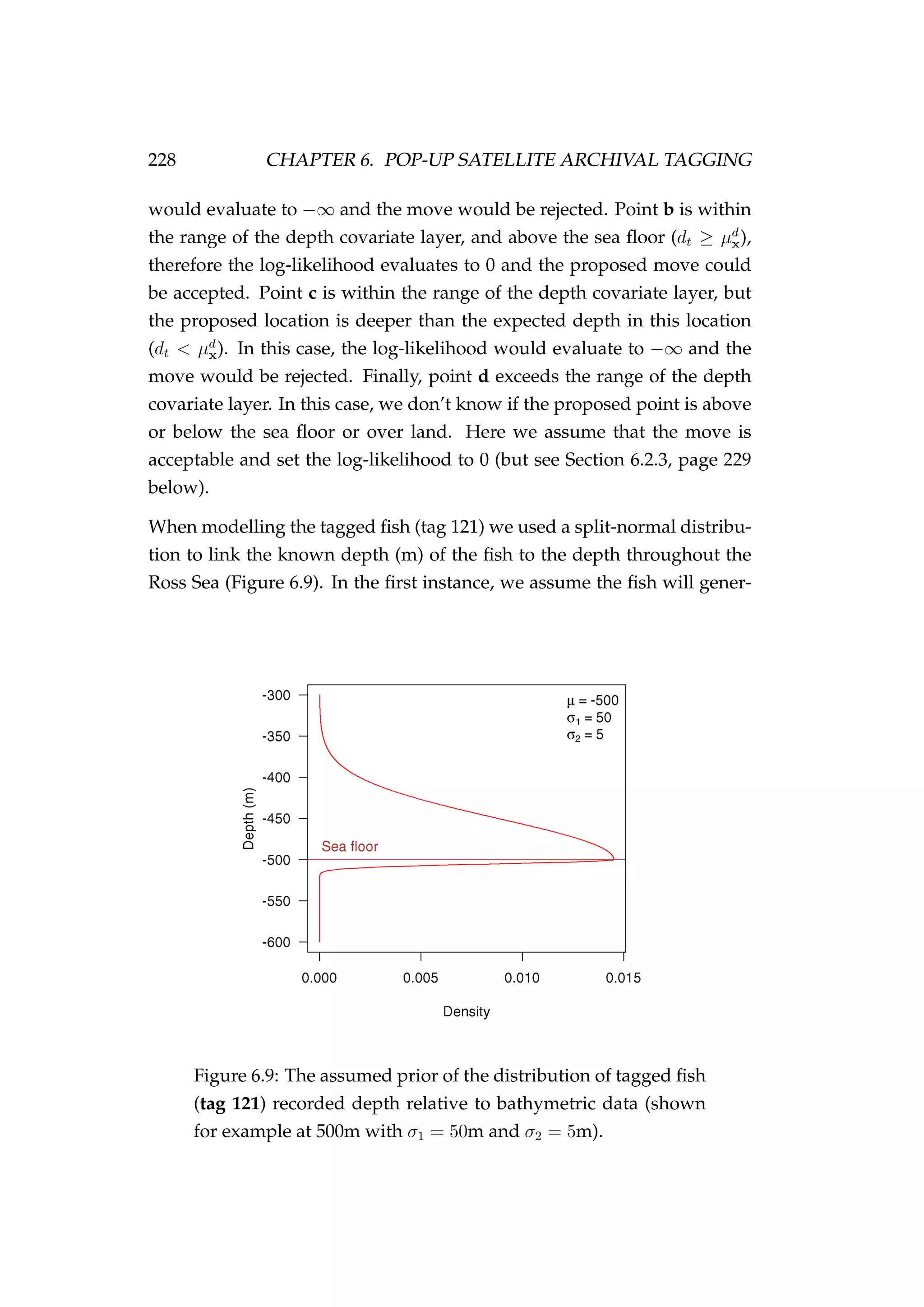
257. 6.6. TAG 121: THE TAGGED FISH 245
where εi represents the unknown error distribution for this model. The
mean distance moved in a single time-step µj
is estimated using linear
regression while fixing the slope at 1
2
(Figure 6.18). The distribution of the
Figure 6.18: Individual time at liberty ti (weeks) versus dis-
tance di (converted to km) travelled between tag-release and
tag-recapture locations using within season recapture data
with the fit of the linear model (Equation 6.16) to these data
shown in red [left], and the distribution of residuals for the fit
εi with the fitted normal distribution in red [right].
residuals εi of this fit informs the prior distribution. We found that εi
iid
∼
N(0, σ2
j ) (Figure 6.18). Therefore the distance moved by a fish in a single
time-step could be expressed as log N µj
, σ2
j where µj
= 9792.331m and
σj = 1.270742m. We can use this knowledge to check that the distances
moved by modelled fish do not greatly exceed what is expected by this
distribution. We also used this information to set an upper bound for the
standard deviation parameter (σx) at 32000m
π (σx) ∼ U (0.001, 32000) . (6.17)
The choice of an upper bound at 3200m is simply three times the mean,
plus a little bit. Therefore, our prior is no longer uninformative.
Both depth and temperature were used to estimate location (Equations 6.7

258. 246 CHAPTER 6. POP-UP SATELLITE ARCHIVAL TAGGING
and 6.11). The model was restricted to be within the bounds of both the
depth and temperature covariate layers. The MCMC for this model was
done in two phases. The first phase involved fitting to temperature and
depth, while turning the log-likelihood contribution of the path off. This
resulted in a path with unrealistically large jumps between locations (e.g.
xt and xt+1) at each time-step in the model. However, it allowed the model
to explore parameter space a lot faster and find locations with suitable
depths and temperature at each time-step. In the second phase, the log-
likelihood contribution of the path was turned on and the MCMC was
run.
Trace plots suggest that the MCMC was mixing well and the samples re-
sulted in reasonable looking posterior distributions, although the poste-
rior for σx was against the upper bound some of the time skewing the
distribution slightly (Figure 6.19). The standard deviation parameter σx
passed the Heidelberger and Welch’s stationarity test and had a Geweke
Z-score of 1.701 (i.e. a p-value of 0.089, only just passed). The distances
moved by the tag between each time-step in the MCMC simulations were
a little higher than those expected (from investigating the distances be-
tween tag-release and tag-recapture of other toothfish tagged in the Ross
Sea, Figure 6.20). This suggests that the upper bound of the uniform prior
on σx could be decreased a little.
The model expected depth of the sea floor was generally not much deeper
than the fish, except in the first four days (Figure 6.21). The model ex-
pected temperature did not agree with the temperature observed by the
tag (Figure 6.22). The model indicated that in the sampled locations and
depths, the temperature should be much lower (about −2◦
C) than that ob-
served by the tag (about 0◦
C). Finally, the estimated path of the tagged
fish (tag 121) is shown in Figure 6.23 below. The hole in the middle of
the paths is largely caused by the bathymetry as it includes depths that
are much greater than those measured toothfish (Figure 6.24). The path
passed the Heidelberger and Welch’s stationarity test at all 2D positions
and resulted in acceptable Z-scores from the Geweke test with 13 points
failing in 1D at the 5% level (Appendix C.4, page 349).

259. 6.6. TAG 121: THE TAGGED FISH 247
Figure 6.19: MCMC trace plots [left] and posterior distributions
[right] and for the standard deviation parameter (σx), the log-
likelihood of the path and the log-likelihood of the data in the
tagged fish (tag 121) model. The log-prior probability density
is not plotted as this was constant.

260. 248 CHAPTER 6. POP-UP SATELLITE ARCHIVAL TAGGING
Figure 6.20: Histogram of the sampled distances (km) between
locations xt and xt+1 for t = 0, . . . , T − 1 at each time-step
and the distance that we might expect a fish to move esti-
mated using alternative information [dashed red line]. The es-
timated parameters of the lognormal distribution shown in red
are given at the top right of the plot.

261. 6.6. TAG 121: THE TAGGED FISH 249
Figure 6.21: Depth (m) of the sea floor under the fish given the
expected path [grey lines] and observed depth of the tagged
fish (tag 121) [+].

262. 250 CHAPTER 6. POP-UP SATELLITE ARCHIVAL TAGGING
Figure 6.22: Sampled temperature (◦
C) expected by the model
given the path [grey lines] and temperature observed by the
tagged fish (tag 121) [•].

263. 6.6. TAG 121: THE TAGGED FISH 251
Figure 6.23: Sampled path taken by the tagged fish (tag 121)
[grey lines], the other two tempered chains β2 = 0.9 [pink lines]
and β3 = 0.8 [cyan lines]. Also shown are the start [•] and end
[•] locations.

264. 252 CHAPTER 6. POP-UP SATELLITE ARCHIVAL TAGGING
Figure 6.24: Bathymetry in the region surrounding the tagged
fish (tag 121). Also shown are the start [•] and end [•] locations.

265. 6.7. DISCUSSION 253
Despite our doubts about the quality of the CARS temperature model, we
attempted to at least try and find a good fit to temperature in the model.
The MCMC was restarted (from the last recorded state in the MCMC sim-
ulation presented above), but the path and depth contribution to the log-
likelihood was turned off (i.e. only the prior and temperature contributed
to the total log-likelihood). Running the model in this way allows the fish
to explore as far as it likes between each time-step, and even explore space
that would otherwise be excluded by the depth data (i.e. we let the fish
cross land). However, the model could not find locations that could match
the two dips in temperature expected by the CARS temperature model.
6.7 Discussion
We have developed novel Bayesian methods for geolocating individual
fish using PSATs. The difference between this model and other models
is that our process model is conditional on x0 and xT . In other words,
we have fixed the start and end location, assuming that they are known
without error. In contrast, other process models may not fix the end point
(often called diffusion models or random walks):
xt
x0 (φ0, λ0)
These models may additionally include some kind of systematic bias or a
“drift” component (advection-diffusion or biased random walks, see Jon-
sen et al. 2013). By fixing the start and the end of the path, we are using
the best two pieces of information we have (the known start and end loca-
tions) to help estimate the path taken by an individual fish and reduce un-
certainty associated with these estimates. Alternatively, one might wish to
admit some uncertainty here (i.e. GPS recorded coordinates do have some
error associated with them), and let the start and end be random variables
but place informed priors on these locations:

266. 254 CHAPTER 6. POP-UP SATELLITE ARCHIVAL TAGGING
xt
π (x0) π (xT )
(φ0, λ0)
In this way, we could admit as little or as much uncertainty about the start
and end locations as is necessary. Or, rather than the process model in
Equation 6.5, we could use
xt|xt−1, xt+1, σx, at ∼ N
1
2
(xt−1 + xt+1) , at
σ2
x
2
I ,
thus scaling the variance by the acceleration at (or we could replace at
with some mean (at−1 + at + at+1)/3). This may help the estimation of the
standard deviation parameter σx. Also, the process model only considers
movement on a 2D horizontal plane. Any vertical movement of the fish
is not captured by the process model and may contribute to the average
total movement of an individual fish within any given time-step (e.g. dis-
tance travelled within a day). This may result in us underestimating the
distance moved by a fish within a time-step. Further improvements to the
process model might include this additional vertical component of the dis-
tance travelled (i.e. a 3D process model). Finally, the process model is set
up as a continuous space, discrete time model. This means that the user
must specify the size of a time-step (e.g. hourly, daily, weekly) and the
data measured by the tag must be aggregated to this temporal resolution.
If using a relatively large time-step then information may be lost. For ex-
ample, the fish may descend to depth for just a single day within a week,
if a weekly time-step is chosen then we may miss this in our model. How-
ever, small time-steps result in the model taking a lot longer to run making
MCMC very slow. Any improvements here might involve changing the
model to a continuous time formulation (i.e. a Markov process model),
using smaller time-steps and investigating the computational potential of
Julia further, summarising the data differently and doing sensitivities (e.g.
doing model runs that use the minimum and maximum depth within a
time-step, rather than just the median), or developing likelihoods that in-
clude variation in the variables measured by the tag as well as the environ-

267. 6.7. DISCUSSION 255
ment (e.g. a likelihood that stipulates that the fish was within some depth
range in any given time-step).
We then develop observation models that attempt to use depth and tem-
perature to geolocate Antarctic toothfish in the Ross Sea. While not en-
tirely successful, the use of depth data to help estimate position is novel.
Our implementation here has made strong assumptions about fish be-
haviour relative to the sea floor. These assumptions may not be valid ex-
cept for species that we are sure are exclusively demersal. It is unlikely that
Antarctic toothfish are exclusively demersal (J. Fenaughty, Pers. Comm.).
Also, we did not include uncertainty in the variables measured by the tag
itself, or incorporate any uncertainty when aggregating the data measured
by the tag (from measurements taken every 16 seconds and 10 minutes to
hourly or weekly time-steps for tag 186 and tag 121 respectively).
The model did not do well in estimating the known path of the towed tag
(tag 186) when fit to the data observed by the tag. In this model, tempera-
ture was the main source of information (depth was only used to exclude
some areas that were too shallow or land). However, the model did very
well in estimating the known path of the tag when the temperature ob-
served by the tag was simulated from the CARS temperature model (and
the standard deviation of temperature was fixed). When the spatially ex-
plicit standard deviation estimates provided by the CARS were used, for
both tag 186 and in the simulation, they resulted in poor estimates of the
known paths. Therefore, the simulation study provides the proof of con-
cept for this modelling framework. However, the method relies on good
data to accurately geolocate fish. The CARS temperature model is inade-
quate for such fine-scale modelling applications. Both the standard devi-
ation estimates and the temperature estimates have proven themselves to
be problematic in trying to geolocate fish.
Light has been used successfully in the past to help estimate a fishes lo-
cation through time (Welch & Eveson 1999). However, toothfish inhabit
deep waters under ice and below the photic zone. In addition, long peri-
ods of constant daylight or constant darkness preclude the use of light for
Antarctic toothfish geolocation year round. Despite this, we recommend

268. 256 CHAPTER 6. POP-UP SATELLITE ARCHIVAL TAGGING
further research to incorporate light and magnetic field strength as addi-
tional observation models. Light could be used to improve the estimates
of location for the towed tag (tag 186), given the strong light signals in
the recorded data (Figure 6.6). However, light would not be useful in es-
timating the location of the actual fish (tag 121). Despite this, light would
be well worth incorporating into this modelling framework if we are to
apply it to other species.
The pattern, or lack of, in total magnetic field strength shown by the
towed tag (tag 186, Figure 6.6) suggests that the pattern shown by tag
121 (Figure 6.7) might be an artifact caused by some other factor (i.e. the
proximity to the sea floor). This discouraged us from using these data
to help improve geolocation of toothfish. While magnetic field strength
was not used here, it may be used successfully elsewhere, particularly
in species with broader spatial ranges (e.g. tuna). It also appears that
the newer versions of the PSAT tags provide more accurate magnetic
field strength data (the technology has improved; K. Echave, K. Coutre
and J. Nielsen Pers. Comm.). Total magnetic field strength is modelled
globally and available by depth and with monthly time steps (https:
//www.ngdc.noaa.gov/geomag/WMM/back.shtml). The best way to
include these information within our modelling framework would be to
call the magnetic field model as sub-models of our model (i.e. the Ju-
lia code accesses the Fortran magnetic field models directly within the
MCMC algorithm). Alternatively, these data may be provided as a grid
in the same way that depth and temperature are used in this chapter.
The implications of this work suggest that the use of PSATs for geolocating
Antarctic toothfish may not be appropriate and perhaps other avenues of
research would be better pursued if geolocation is the goal (e.g. acoustic
tagging). However, discussions with NOAA scientists (K. Echave and K.
Coutre) and J. Neilsen suggest that the technology has improved in the
newer tags and that they provide more accurate magnetic field strength
and acceleration data. Therefore, we recommend that more tags be placed
on Antarctic toothfish so that magnetic field strength data can be utilised
within the modelling framework. With the addition of light and magnetic
field observation models, this modelling framework could be a powerful

269. 6.7. DISCUSSION 257
tool for other species as well.

270. 258 CHAPTER 6. POP-UP SATELLITE ARCHIVAL TAGGING

271. Chapter 7
Bayesian emulation
In this chapter we develop Bayesian emulators for practical applications
in fisheries research and provide examples. We begin by introducing de-
terministic univariate emulators. We then extend the emulation frame-
work to include stochasticity and develop a stochastic multivariate emu-
lator of an agent-based model (ABM) of snapper in northern New Zealand
(Pagurus auratus, SNA 1, for more information on snapper see Chapter 3,
page 77) as described in Chapter 4.
7.1 Introduction
Complex models can be computationally expensive, taking many hours or
days to do a single run. Models of this ilk make inference using standard
methods impractical. For example, the ABM described in Chapter 4 takes
about 16 hours to do a single run (for the snapper example). Attempting to
use standard MCMC methods for relatively few samples from the poste-
rior distribution of this model, say 1000 samples with no thinning, would
take about two years.
However, methods do exist for speeding up inference of such computa-
tionally expensive models. In Chapter 2 (page 71) we briefly described
approximate Bayesian computation (ABC) and Bayesian emulation as fea-
sible alternatives for Bayesian inference in complex models. In this chapter
259

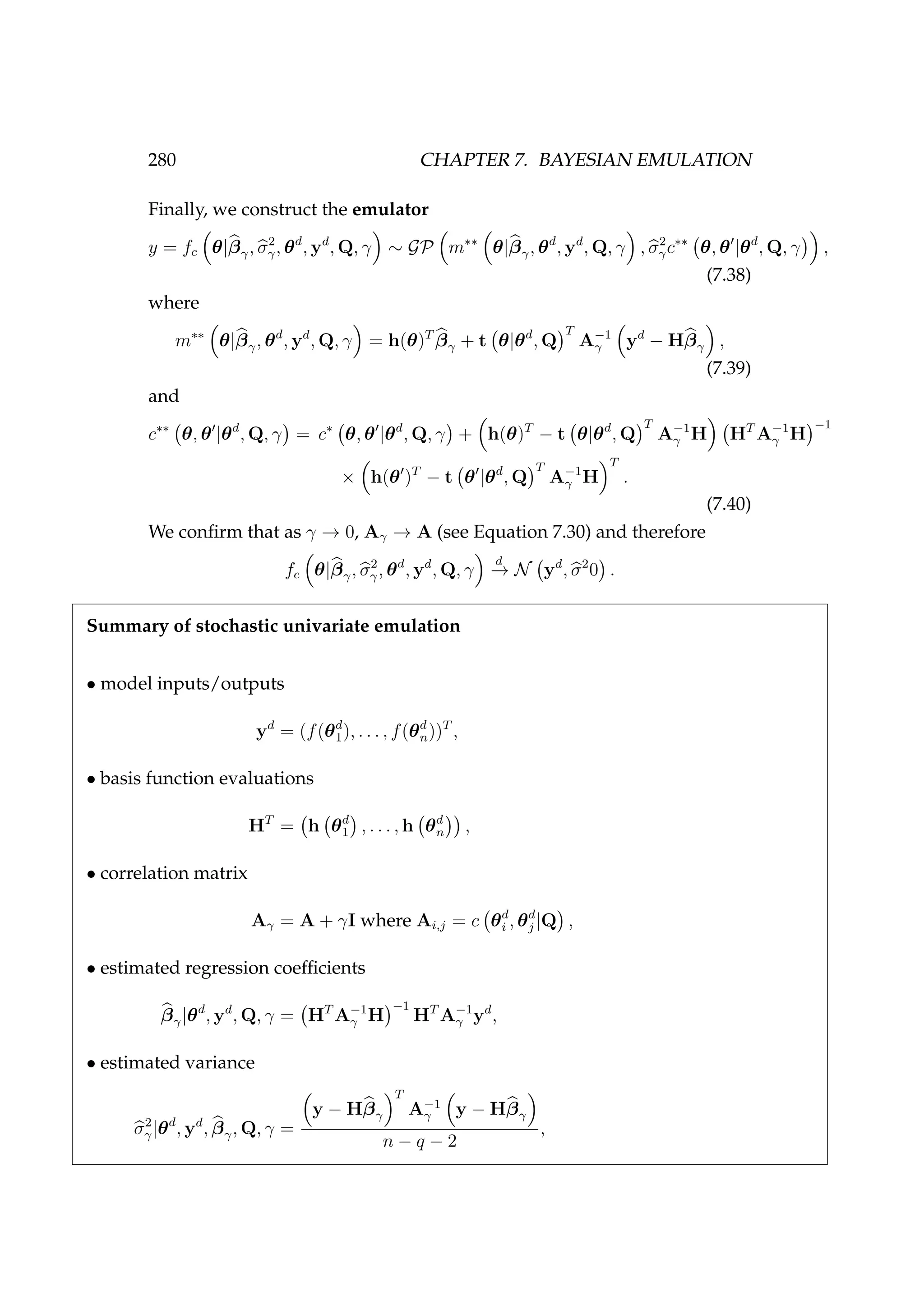
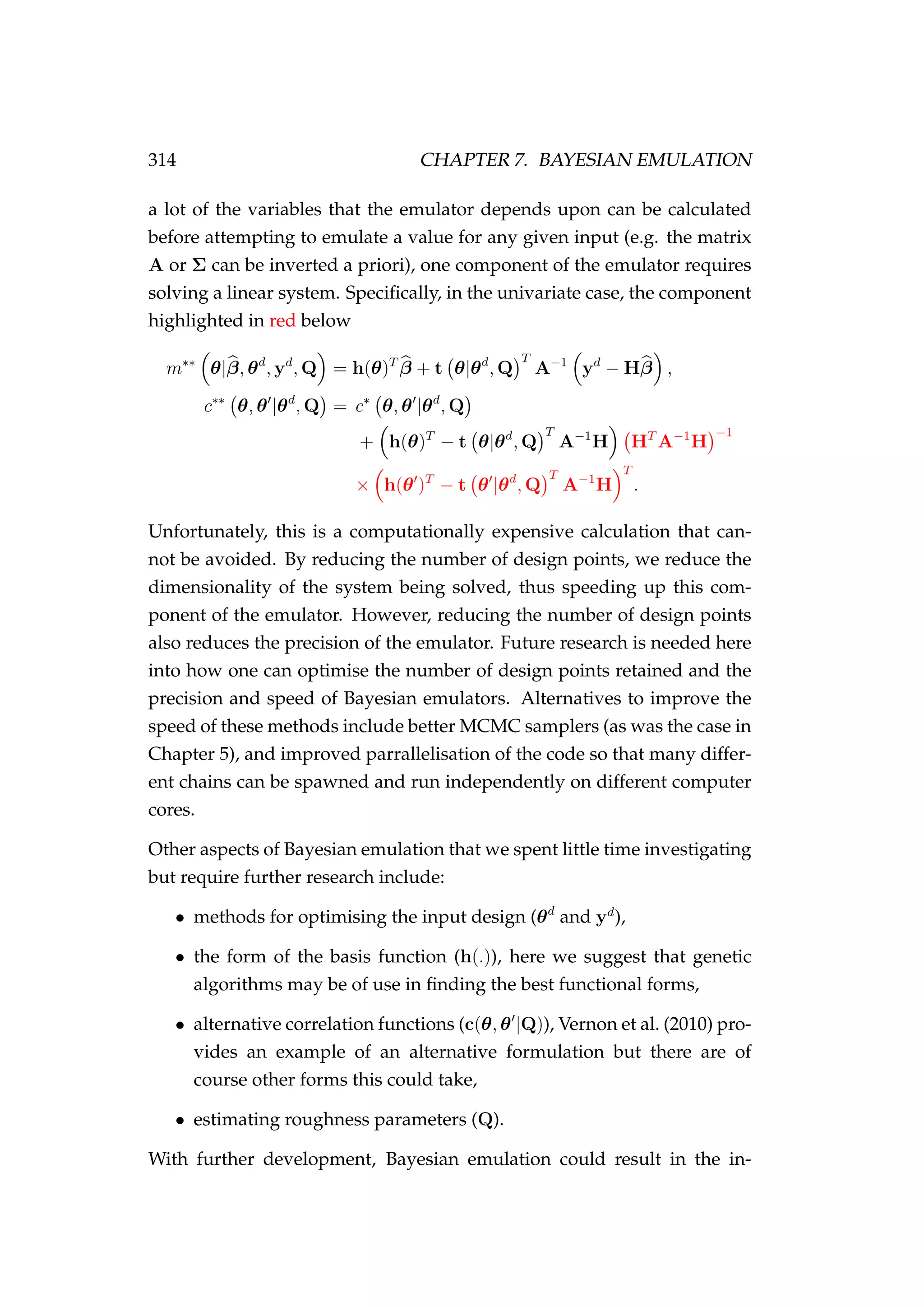
272. 260 CHAPTER 7. BAYESIAN EMULATION
we cover Bayesian emulation in more detail, extend the method beyond
what is currently described in the literature (e.g. Goldstein & Rougier 2006,
Hankin 2005, Oakley & O’Hagan 2004), and apply the method to fisheries
problems.
A Bayesian emulator’s task is to quickly estimate a function f(θ) for an
arbitrary value of its argument θ. This might be achieved by drawing
a smooth curve through a set of design points (θi, f(θi)) and using this
curve to predict f(θ) for any θ. If the desired θ is in between the largest
and smallest of the θi’s the problem is called interpolation, if θ is outside
that range it is called extrapolation. Of course, care must be taken when
choosing a set of design points (θi’s) so as to avoid extrapolation, because
estimates of f(θ) beyond θi can be unstable (e.g. Figure 7.1). Interpolation
Figure 7.1: The fit of a third order polynomial [solid red line]
and a sixth order polynomial [dashed green line] to the points
a to o.
is related to, but distinct from, function approximation. This consists of
finding an approximate (but easily computable) function to use in place
of a more complicated one. In the case of interpolation we know the out-
put of function f(·) at points that may not be of our choosing or limited
to a smaller set than desired. In function approximation the function f(·)
can be computed at any desired points for the purpose of developing our
approximation. See Chapter 3 of Press et al. (1986) for more detail on inter-
polation and extrapolation and Chapter 5 for details on function approxi-

273. 7.1. INTRODUCTION 261
mation.
Bayesian emulation includes aspects of interpolation/extrapolation and
function approximation. Furthermore, an emulator acts both as an ap-
proximation to the function and as an assessment of the uncertainty intro-
duced by the approximation. Bayesian emulation coupled with Bayesian
inference provides a method for making inference of computationally ex-
pensive computer models tractable (e.g. Henderson et al. 2009) as a good
emulator will be much faster than the model it is emulating.
A univariate emulator provides an approximation to a function that takes
multiple input parameters (θ)1
and returns a scalar output (y)
y = f(θ).
A multivariate emulator is a generalisation of a univariate emulator and
provides an approximation to a function that takes multiple input param-
eters (θ) and returns a vector of outputs (y)
y = f(θ).
Bayesian emulators are based on Gaussian processes (GP). A Gaussian
process is a type of stochastic process in which every point in some input
space is associated with a normally distributed random variable and any
collection of those random variables is multivariate normal. If we write
g(x) ∼ GP (m(x), c(x, ·)) ,
then we are stating that the random function g(x) is distributed as a Gaus-
sian process with mean function m(x) and covariance function c(x, ·).
Therefore, by the definition of Gaussian processes, if we take any set
T : (t1, . . . , tT ) then x = (x1, . . . , xT ) is multivariate normal
x ∼ N (µ, Σ) ,
with µt = m(xt) and Σt,t = c(t, t ) for t, t ∈ {1, . . . , T }.
1
Actually, an emulated function could take a single input parameter (θ). We provide
an example of this in Section 7.2.2 (page 275).

274. 262 CHAPTER 7. BAYESIAN EMULATION
Computationally expensive models are common in many scientific disci-
plines including fisheries science. However, thus far there have been very
few applications of Bayesian emulation in the literature (but see Vernon
et al. 2010 which applies the method to a galaxy formation model). In-
deed, the method has not been applied in fisheries despite the fact that
we commonly encounter computationally expensive models that preclude
the use of standard Bayesian inference methods. Examples of these com-
plex models include the likes of Atlantis (http://www.cmar.csiro.
au/research/mse/atlantis.htm) and InVitro (Gray et al. 2006, Little
et al. 2006). Therefore, in this chapter we further develop Bayesian emula-
tors in the fisheries context, and provide a proof of concept for their use in
complex fisheries settings.
7.2 Univariate emulators
A list of the variables used in describing univariate emulators is provided
in Tables 7.1 and 7.2. We define the parameters, or inputs, of a computer
model to be some vector θ = {θj}p
j=1, and the output of the model to be a
scalar y. We represent the computer model as some deterministic function
f(·), thus
y = f(θ).
By deterministic we mean that the same input (θ) always yields the iden-
tical output (y). In Section 7.3 (page 278) below we relax this requirement
so that we can emulate stochastic simulation models.
Our goal is to estimate θ∗
, the “true” value(s) of the inputs conditional on
some data or observations. We define y∗
to be the output of the model
when θ∗
is the input, thus
y∗
= f(θ∗
).
If f(·) is computationally expensive, then finding θ∗
using standard infer-
ence methods can be impractical.
Instead, we approximate f(θ) by a Gaussian process
y = h(θ)T
β + ε(θ)

275. 7.2. UNIVARIATE EMULATORS 263
Table 7.1: Notation used in discussing and defining Bayesian emulation.
The inputs and outputs of a computer model.
Symbol Type Dimension Description
n scalar 1 Number of design points i ∈ n
p scalar 1 Dimension of input space j ∈ p
q scalar 1 Number of regression functions k ∈ q
Θ vector p The input space
θ vector p × 1 An element of the input space θ = {θj}p
j=1
where θ ∈ Θ
θd
matrix n × p Matrix of inputs θd
= {θd
i }n,p
i=1,j=1 for which
we have outputs yd = {yd
i }n
i=1
θ vector p × 1 Vector of inputs for which an output is to be
approximated
θ∗
vector p × 1 The true value of θ
yd vector n × 1 Vector of outputs at the design points yd =
{yd
i }n
i=1
y scalar 1 The approximation of y given the vector of in-
puts θ
y∗ scalar 1 The true value of y
yo scalar 1 Observed data

276. 264 CHAPTER 7. BAYESIAN EMULATION
Table 7.2: Notation used in discussing and defining Bayesian emulation.
The emulator.
Symbol Type Dimension Description
n scalar 1 Number of design points i ∈ n
p scalar 1 Dimension of input space j ∈ p
q scalar 1 Number of regression functions
k ∈ q
β vector q × 1 Vector of regression coefficients
β vector q × 1 The estimated value of β updated
in light of the design outputs yd
σ2
e scalar 1 Emulator variance
σ2
e scalar 1 A posteriori estimate for the vari-
ance
h(θ) vector q × 1 Basis function
H matrix n × q Matrix of basis function values
evaluated at each input θd
(from
simulator)
Q matrix p × p Diagonal matrix of roughness pa-
rameters
c(θ, θ |Q) scalar 1 Correlation function
A matrix n × n Correlation matrix
t(θ|θd
, Q) vector n × 1 Vector of covariances between θ
and θd
m∗(θ|β, θd
, yd, Q) scalar 1 Prior expectation
m∗∗(θ|β, θd
, yd, Q) scalar 1 A posteriori expectation
c∗(θ, θ |θd
, Q) scalar 1 Prior variance
c∗∗(θ, θ |θd
, Q) scalar 1 A posteriori variance

277. 7.2. UNIVARIATE EMULATORS 265
where
ε(θ) ∼ GP 0, σ2
c(θ, θ |Q) .
We explain each of the components of this approximation and the con-
struction of an emulator in more detail below.
By running the computer model relatively few times we can generate a set
of model outputs (yd
i ’s) for a set of design points (θd
i )
yd
i = f(θd
i ) where i = 1, . . . , n,
yd
= (yd
1, . . . , yd
n)T
, (7.1)
where n is the number of design points. The design points are chosen
such that they are spread to adequately cover Θ, the input space of θ.
McKay et al. (1979) propose the use of Latin hypercube sampling. Sup-
pose θ = (θ1, . . . , θp) and we wish to draw n random values for θ. For
j = 1, . . . , p, we divide the sample space of θj into n regions of equal
marginal probability. This requires the specification of a prior for θ in
advance and this prior should not be too diffuse. Here we simply use a
uniform prior within a fixed range. We then draw one random value of θi
from each region. This process is repeated, sampling without replacement
for i = 1, . . . , n. This ensures that each dimension of the input space is bet-
ter represented than sampling from a uniform distribution for each input
parameter (θj) independently.
As mentioned earlier, we approximate f(θ) by a Gaussian process
y = fa(θ|β, σ2
e , Q) ∼ GP m(θ|β), σ2
e c(θ, θ |Q) ,
E[y] = E fa(θ|β, σ2
e , Q) = m(θ|β) = h(θ)T
β, (7.2)
conditional on the unknown vector of coefficients β = {βk}q
k=1. The vector
h(·) is referred to as the basis function and consists of q known regression
functions of θ = (θ1, . . . , θp)T
. The choice of h(·) should incorporate any
knowledge we have about f(·). A common choice is simply the set of
linear functions h(θ) = (1, θ1, . . . , θp)T
, but other functions of θ may be
chosen2
.
2
Note that we do not change the symbol y here or in the following pages (i.e. when
stating y = fa(θ), y = fu(θ) or y = fc(θ)) because we are sequentially building up the
way in which we emulate y.

278. 266 CHAPTER 7. BAYESIAN EMULATION
We now consider how we expect the approximation h(θ)T
β to deviate
from f(θ). By the definition of the Gaussian process the covariance be-
tween fa(θ|β, σ2
e , Q) and fa(θ |β, σ2
e , Q) is given by
C fa(θ|β, σ2
e , Q), fa(θ |β, σ2
e , Q) = σ2
e c(θ, θ |Q), (7.3)
conditional on a constant variance parameter σ2
e , where c(θ, θ |Q) is a cor-
relation function that measures the correlation between f(·) at θ and θ
conditional on a set of roughness parameters (Q). The function c(θ, θ |Q)
decreases as |θ − θ | increases, satisfies c(θ, θ|Q) = 1 ∀θ, and must en-
sure that the covariance matrix of any set of outputs {y1 = f(θ1), . . . , yn =
f(θn)} is positive semi-definitive. A typical choice is
c(θ, θ |Q) = exp −(θ − θ )T
Q(θ − θ ) , (7.4)
where Q is a p × p diagonal matrix of roughness scales3
. This form has
the advantage that f(·) has derivatives of all orders; other forms for the
covariance function may not have this desirable property (Oakley 1999).
The Gaussian process (Equation 7.2) implies that on the design points our
data can be approximated by
yd
∼ N Hβ, σ2
e A , (7.5)
where
HT
= h θd
1 , . . . , h θd
n , (7.6)
Ai,j = c θd
i , θd
j |Q , (7.7)
with Ai,j = Aj,i and Aj,j = 1. More explicitly
A =







1 c θd
1, θd
2|Q · · · c θd
1, θd
n|Q
c θd
2, θd
1|Q 1
...
...
...
c θd
n, θd
1|Q · · · 1







.
3
Vernon et al. (2010) provides an example of an alternative formulation
c(θ, θ |Q) = exp − θ − θ
2
/Q2
that we do not use here.

279. 7.2. UNIVARIATE EMULATORS 267
We then calibrate the approximation by finding the restricted maximum
likelihood (REML) estimates of β and σ2
e using standard methods (Diggle
et al. 2002, Marin & Robert 2010, Patterson & Thompson 1971)
β θd
, yd
, Q = HT
A−1
H
−1
HT
A−1
yd
, (7.8)
σ2
e θd
, yd
, Q =
yd T
A−1
− A−1
H HT
A−1
H
−1
HT
A−1
yd
n − q
. (7.9)
Using weak prior distributions for β and σ2
e
π (β) ∝ 1,
π σ2
e ∝
1
σ2
e
,
or
π β, σ2
e ∝ σ−2
e , (7.10)
and combining with Equation 7.5 using Bayes’ theorem we derive the pos-
terior4
. First we define the independent residual projection matrix (G)
G = I − H HT
A−1
H
−1
HT
A−1
GH = H − H HT
A−1
H
−1
HT
A−1
H = 0
e = Gyd
= yd
− Hβ,
from which it follows that
yd
− Hβ = yd
− Hβ + H β − β
= yd
− H HT
A−1
H
−1
HT
A−1
yd
+ H β − β
= Gyd
+ H β − β
yd
− Hβ
T
A−1
yd
− Hβ = Gyd
+ H β − β
T
A−1
Gyd
+ H β − β
= yd
GT
A−1
Gyd
+ β − β
T
HT
A−1
H β − β
+ β − β
T
HT
A−1
Gyd
= eT
A−1
e + β − β
T
HT
A−1
H β − β + 0,
4
Note that the prior π (Q) is left unspecified.

280. 268 CHAPTER 7. BAYESIAN EMULATION
and
σ2
e =
eT
A−1
e
n − q
The posterior for β, σ2
e and Q given the design data yd
is therefore
p β, σ2
e , Q|yd
∝ p yd
|β, σ2
e , Q π(β)π σ2
e π (Q)
∝
1
σ2
e
p yd
|β, σ2
e , Q π (Q) using Equation 7.10
∝
1
σ2
e
(2πσ2
e )−n
2 |A|−1
2 exp −
1
2σ2
e
yd
− Hβ
T
A−1
yd
− Hβ π (Q)
using Equation 7.5
∝ σ2
e
−(n+2
2 )
|A|−1
2 exp −
1
2σ2
e
yd
− Hβ
T
A−1
yd
− Hβ π (Q)
∝ σ2
e
−(n+2
2 )
|A|−1
2 exp −
1
2σ2
e
eT
A−1
e + β − β
T
HT
A−1
H β − β π (Q)
∝ p β|σ2
e , Q, yd
p σ2
e |Q, yd
p Q|yd
∝ 2πσ2
e
− q
2
HT
A−1
H
1
2
exp
1
2σ2
e
β − β
T
HT
A−1
H β − β
× σ2
e
−(n−q
2 )−1
exp −
1
2σ2
e
eT
A−1
e
1
2
eT
A−1
e
n−q
2
Γ n−q
2
× |A|−1
2 |HT
A−1
H|−1
2
1
2
eT
A−1
e
−(n−q
2 )
π (Q) .
This can be split up into the components that we are interested in
p β|σ2
e , Q, yd
= 2πσ2
e
− q
2
|HT
A−1
H|
1
2 exp −
1
2σ2
e
β − β
T
HT
A−1
H β − β ,
(7.11)
p σ2
e |Q, yd
=
1
2
eT
A−1
e
n−q
2
Γ n−q
2
σ2
e
−n−q
2
−1
e
− 1
σ2
e
(−1
2
eT A−1e)
, (7.12)
p Q|yd
∝ σ2
e
−n−q
2
|A|−1
2 HT
A−1
H
−1
2
π (Q) . (7.13)
Equation 7.13 defines the posterior distribution for the roughness scales
(Q). The roughness scales are known to be difficult to estimate (Kennedy
& O’Hagan 2000, Oakley 2004). In practice, the roughness scales are ei-
ther fixed by assumption, or are estimated by maximising, over allowable
scales, the posterior assuming a uniform prior π(Q) ∝ 1
f(Q|yd
) ∝ σ2
e
−n−q
2
|A|−1
2 HT
A−1
H
−1
2
. (7.14)

281. 7.2. UNIVARIATE EMULATORS 269
Therefore, the Bayesian posteriors for β and σ2
e , conditional on θd
, yd
and
the roughness scales (Q), are
β|σ2
e , θd
, yd
, Q ∼ N β, σ2
e HT
A−1
H
−1
, (7.15)
σ2
e |θd
, yd
, Q ∼ IG
n − q
2
,
1
2
eT
A−1
e . (7.16)
Next, we construct an approximation fu θd
i |β, σ2
e , θd
, yd
, Q constrained
such that yd
i = fu θd
i |β, σ2
e , θd
, Q and V yd
i = 0 given the true values
of β and σ2
e , the design inputs (θd
), and the roughness matrix (Q). This
is accomplished by considering the joint distribution of yd
and a further
observation y and input θ
y
yd
∼ N
h(θ)T
β
Hβ
,
σ2
σ2
t(θ|θd
, Q)T
σ2
t(θ|θd
, Q)T
σ2
A
,
where
t(θ|θd
, Q)T
= c(θ, θd
1|Q), . . . , c(θ, θd
n|Q) . (7.17)
A standard result for multivariate normal distributions (Theorem 4.4
in Rencher 2000) states that if
x1
x2
∼ N
µ1
µ2
,
Σ1,1 Σ1,2
Σ2,1 Σ2,2
,
then
x1|x2 ∼ N µ1 + Σ1,2Σ−1
2,2 (x2 − µ2) , Σ1,1 − Σ1,2Σ−1
2,2Σ2,1 .
Therefore
y|θ, θd
, yd
, β, σ2
, Q ∼ GP h(θ)T
β − t(θ|θd
, Q)T
A−1
yd
+ Hβ ,
σ2
1 − t(θ|θd
, Q)T
A−1
t(θ |θd
, Q)T
.
If we define
m∗
θ|β, θd
, yd
, Q = h(θ)T
β + t θ|θd
, Q
T
A−1
yd
− Hβ , (7.18)
c∗
θ, θ |θd
, Q = c (θ, θ |Q) − t(θ|θd
, Q)T
A−1
t(θ |θd
, Q), (7.19)

282. 270 CHAPTER 7. BAYESIAN EMULATION
then we can write
y = fu θ|β, σ2
e , θd
, yd
, Q ∼ GP m∗
θ|β, θd
, yd
, Q , σ2
e c∗
θ, θ |θd
, Q .
(7.20)
We now verify that if θ = θd
i then E fu θd
i |β, σ2
e , θd
, yd
, Q = yd
i and
V fu θd
i |β, σ2
e , θd
, yd
, Q = 0 (i.e. the emulator matches the simulator
exactly and the variance is zero)
E fu θd
i |β, σ2
e , θd
, yd
, Q = m∗
θd
i |β, θd
, yd
, Q
= h(θd
i )T
β + t θd
i |θd
, Q
T
A−1
yd
− Hβ
= h(θd
i )T
β + δT
i yd
− Hβ
= h(θd
i )T
β + δT
i yd
− δT
i Hβ
= h(θd
i )T
β + yd
i − h(θd
i )T
β
= yd
i ,
and
V fu θd
i |β, σ2
e , θd
, yd
, Q = σ2
e c∗
θd
i , θd
i |θd
, Q
= σ2
e c θd
i , θd
i |Q − t θd
i |θd
, Q
T
A−1
t θd
i |θd
, Q
= σ2
e 1 − δT
i t(θd
i |θd
, Q) = σ2
e 1 − c θd
i , θd
i |Q
= σ2
e (1 − 1)
= 0.
Here δT
i is a vector of length n containing all zeros except that element
i is equal to one. In words, both Equations 7.18 and 7.19 consist of two
components. In Equation 7.18, the first component h(θ)T
β is our prior ex-
pectation of f(·), which conditional on β is h(θ)T
β. The expected value of
β has been updated in light of the outputs yd
. The second component
t θ|θd
, Q
T
A−1
yd
− Hβ adjusts the posterior mean so that it passes
exactly through all of the outputs (i.e. if we have observed the output
yd
i = fu θd
i |β, σ2
e , θd
, Q , then E fu θd
i |β, σ2
e , θd
, Q = yd
i ). How smoothly
m∗
(·) departs from h(θ)T
β towards any observed output yd
i for θ close to
θd
i will depend on Q. In Equation 7.19, the first component c(θ, θ |Q) is the
correlation function. The second component, t(θ|θd
, Q)T
A−1
t(θ |θd
, Q)
adjusts the variance so that it is equal to zero if f(θ) is known.

283. 7.2. UNIVARIATE EMULATORS 271
Finally, we combine Equations 7.15 and 7.20 and integrate out β, using its
posterior (Equation 7.15), to construct the emulator
E y|yd
, Q = E E y|β, σ2
e , yd
, Q yd
, Q
= E m∗
(θ) yd
, Q
= E h (θ)T
β − t(θ|θd
, Q)T
A−1
yd
− Hβ
= h (θ)T
E [β] − t(θ|θd
, Q)T
A−1
yd
− HE [β]
= h (θ)T
β − t(θ|θd
, Q)T
A−1
yd
− Hβ ,
V y|yd
, Q = E V y|β, σ2
e , yd
, Q yd
, Q + V E y|β, σ2
e , yd
, Q yd
, Q
= E σ2
e c (θ, θ |Q) − t(θ|θd
, Q)T
A−1
t(θ |θd
, Q) yd
, Q
+ V h (θ)T
β + t(θ|θd
, Q)T
A−1
yd
− Hβ |yd
, Q
= E σ2
e |yd
, Q c (θ, θ |Q) − t(θ|θd
, Q)T
A−1
t(θ |θd
, Q)
+ V h (θ)T
− t(θ|θd
, Q)T
A−1
H β + t(θ|θd
, Q)T
yd
yd
, Q
= σ2
e c (θ, θ |Q) − t(θ|θd
, Q)T
A−1
t(θ |θd
, Q)
+ h (θ)T
− t(θ|θd
, Q)T
A−1
H V β|yd
, Q h (θ)T
− t(θ|θd
, Q)T
A−1
H
T
= σ2
e c (θ, θ |Q) − t(θ|θd
, Q)T
A−1
t(θ |θd
, Q)
+ h (θ)T
− t(θ|θd
, Q)T
A−1
H HT
A−1
H
−1
h (θ)T
− t(θ|θd
, Q)T
A−1
H
T
Therefore, we write
y ∼ GP m∗∗
θ |β, θd
, yd
, Q , σ2
e c (θ, θ |Q) ,
or
y = fc θ|β, σ2
e , θd
, yd
, Q ∼ GP m∗∗
θ|β, θd
, yd
, Q , σ2
e c∗∗
θ, θ |θd
, Q ,
(7.21)
where
m∗∗
θ |β, θd
, yd
, Q = h(θ )T
β + t θ|θd
, Q
T
A−1
yd
− Hβ , (7.22)
c∗∗
θ, θ |θd
, Q = c∗
θ, θ |θd
, Q + h(θ)T
− t θ|θd
, Q
T
A−1
H HT
A−1
H
−1
× h(θ )T
− t θ |θd
, Q
T
A−1
H
T
.
(7.23)

284. 272 CHAPTER 7. BAYESIAN EMULATION
To summarise, a Bayesian emulator provides an approximation of a com-
puter model f(·). An emulator for f(·) is specified by a choice of regressors
h(θ) and a choice of correlation function c(θ, θ |Q). The emulator is con-
ditioned, or trained, using a relatively small set of evaluations of f(·), i.e.
yd
= f(θd
), given a carefully selected set of inputs θd
. The conditioning
process updates our estimates of the vector β, the scalar σ2
e and is used to
estimate the matrix Q. The design points θd
and yd
are also used during
evaluations of the emulator to interpolate (or extrapolate) a value for y
given a vector of inputs θ .
Therefore, the construction of a Bayesian emulator involves the following
steps:
1. Develop a sample design (θd
)
2. Evaluate yd
= f(θd
)
3. Decide on a basis function (h(θ))
4. Decide on a correlation function (c(θ, θ |Q)) and estimate the rough-
ness scales (Q)
5. Condition the emulator
The conditioned emulator may then be used for anything that the original
function f(·) could be used for, including model evaluation, simulation,
or inference.
Summary of deterministic univariate emulation
• model inputs/outputs
yd
= (f(θd
1), . . . , f(θd
n))T
,
• basis function evaluations
HT
= h θd
1 , . . . , h θd
n ,
• correlation matrix
Ai,j = c θd
i , θd
j |Q ,

285. 7.2. UNIVARIATE EMULATORS 273
• estimated regression coefficients
β|θd
, yd
, Q = HT
A−1
H
−1
HT
A−1
yd
,
• estimated variance
σ2
e |θd
, yd
, Q =
yd T
A−1
− A−1
H HT
A−1
H
−1
HT
A−1
yd
n − q − 2
,
• a posteriori expectation
t(θ|θd
, Q)T
= c(θ, θd
1|Q), . . . , c(θ, θd
n|Q) ,
m∗∗
θ |β, θd
, yd
, Q = h(θ )T
β + t θ|θd
, Q
T
A−1
yd
− Hβ ,
• a posteriori covariance
c∗∗
θ, θ |θd
, Q = c∗
θ, θ |θd
, Q + h(θ)T
− t θ|θd
, Q
T
A−1
H HT
A−1
H
−1
× h(θ )T
− t θ |θd
, Q
T
A−1
H
T
.
7.2.1 A one-dimensional example
To illustrate some of the details of standard univariate Bayesian emulation,
we begin with a simple one-dimensional example (i.e. a single input θ and
a single output y). We define the function
f(θ) ∼



0 θ ≤ 0.5
1 θ > 0.5
, (7.24)
where 0 ≤ θ ≤ 1. We set θd
= {θd
i }n
i=1 as 10 evenly spaced points from
0 to 1 (i.e. n = 10). Outputs are simulated from Equation 7.24 for yd
=
{yd
i }n
i=1 = f(θd
). A set of four emulators are then conditioned on θd
and yd
by selecting n = {5, 7, 8, 10} design points from the total of 10 above. The
basis function h(θ) = (1, cos(θ)) is used for all four emulators. We would

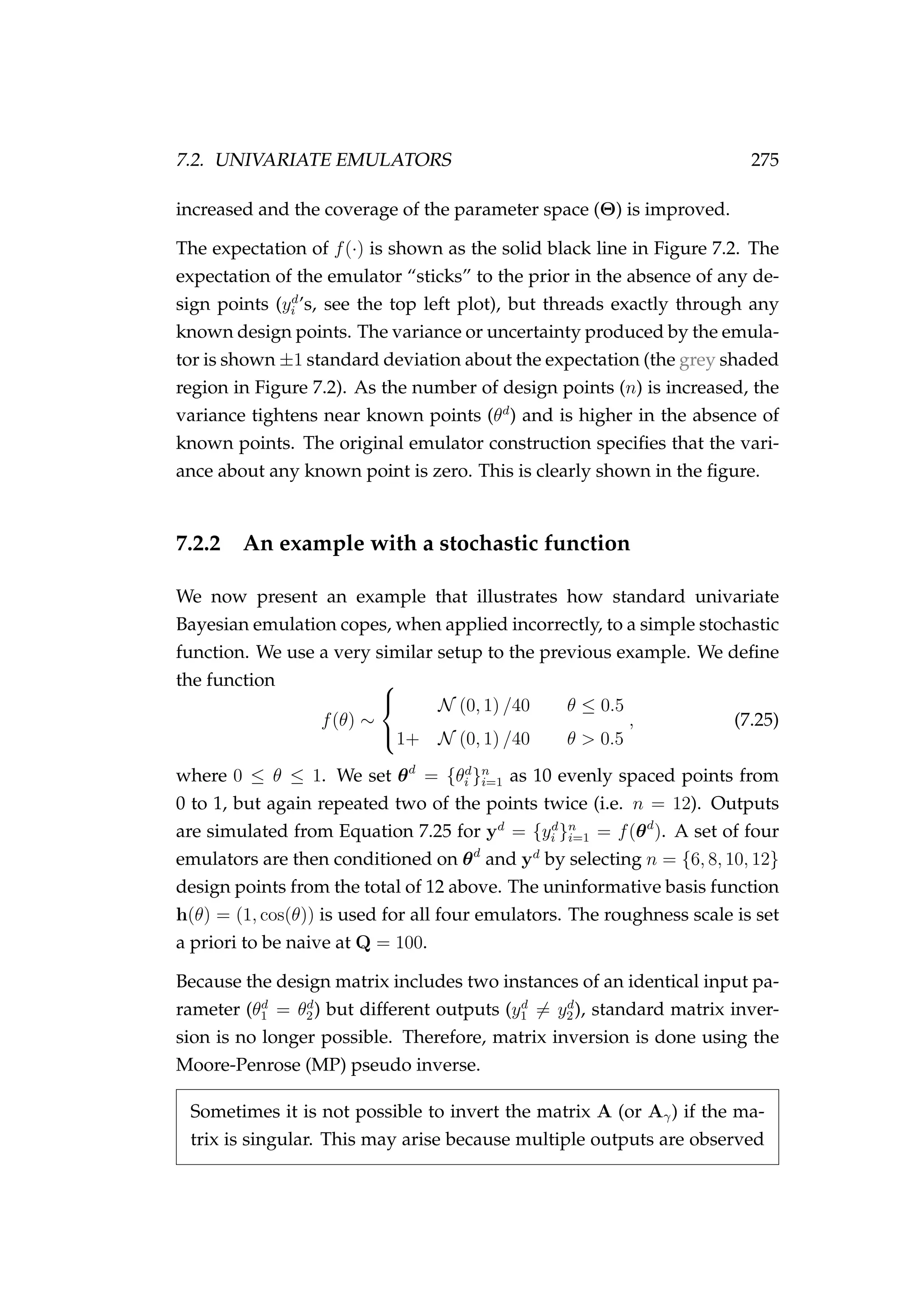
286. 274 CHAPTER 7. BAYESIAN EMULATION
not expect this basis function to do a very good job of emulating the step
function above. The roughness scale is set a priori to be uninformative at
Q = 100.
The emulator is then used to make inference about f(θ ) for θ = 0, . . . , 1
(Figure 7.2). This example illustrates how the basis function (h(θ)) forms
Figure 7.2: A sequence of emulators conditioned on θd
=
{θd
i }n
i=1 and yd
= {yd
i }n
i=1 for n = {6, 8, 10, 12} design points. In
each plot θd
is the training set or model input plotted against
the model output [•]. m∗∗
(·) is the best estimate [solid line], ±1
standard deviation [grey band], and h(θ)β is the prior [dashed
red line].
the prior (h(θ)β, shown as the dashed red line in Figure 7.2), and how this
prior is updated as the number of inputs (n) are increased from n = 6 to
n = 12. It also illustrates how the prior becomes less important as n is

287. 7.2. UNIVARIATE EMULATORS 275
increased and the coverage of the parameter space (Θ) is improved.
The expectation of f(·) is shown as the solid black line in Figure 7.2. The
expectation of the emulator “sticks” to the prior in the absence of any de-
sign points (yd
i ’s, see the top left plot), but threads exactly through any
known design points. The variance or uncertainty produced by the emula-
tor is shown ±1 standard deviation about the expectation (the grey shaded
region in Figure 7.2). As the number of design points (n) is increased, the
variance tightens near known points (θd
) and is higher in the absence of
known points. The original emulator construction specifies that the vari-
ance about any known point is zero. This is clearly shown in the figure.
7.2.2 An example with a stochastic function
We now present an example that illustrates how standard univariate
Bayesian emulation copes, when applied incorrectly, to a simple stochastic
function. We use a very similar setup to the previous example. We define
the function
f(θ) ∼



N (0, 1) /40 θ ≤ 0.5
1+ N (0, 1) /40 θ > 0.5
, (7.25)
where 0 ≤ θ ≤ 1. We set θd
= {θd
i }n
i=1 as 10 evenly spaced points from
0 to 1, but again repeated two of the points twice (i.e. n = 12). Outputs
are simulated from Equation 7.25 for yd
= {yd
i }n
i=1 = f(θd
). A set of four
emulators are then conditioned on θd
and yd
by selecting n = {6, 8, 10, 12}
design points from the total of 12 above. The uninformative basis function
h(θ) = (1, cos(θ)) is used for all four emulators. The roughness scale is set
a priori to be naive at Q = 100.
Because the design matrix includes two instances of an identical input pa-
rameter (θd
1 = θd
2) but different outputs (yd
1 = yd
2), standard matrix inver-
sion is no longer possible. Therefore, matrix inversion is done using the
Moore-Penrose (MP) pseudo inverse.
Sometimes it is not possible to invert the matrix A (or Aγ) if the ma-
trix is singular. This may arise because multiple outputs are observed

288. 276 CHAPTER 7. BAYESIAN EMULATION
given the same inputs (i.e. θd
i = θd
j but yd
i = yd
j ). This cannot happen
under a deterministic model, but it may occur if a model is stochas-
tic. When this occurs the Moore-Penrose generalised pseudo-inverse
of a matrix (A+
) can be used to solve the matrix (Moore 1920, Penrose
1955). The Moore-Penrose pseudo-inverse has the following proper-
ties:
• If A is invertible, its pseudo-inverse is its inverse A+
= A−1
• The pseudo-inverse of the pseudo-inverse is the original matrix
(A+
)+
= A
• Pseudo-inversion commutes with transposition, conjugation,
and taking the conjugate transpose (AT
)+
= (A+
)T
, A
+
=
A+, (A∗
)+
= (A+
)∗
.
The emulator is used to make inference about f(θ ) for θ = 0, . . . , 1 (Fig-
ure 7.3). As in the previous example, this example illustrates how the ba-
sis function (h(θ)) forms the prior (h(θ)β, shown as the dashed red line in
Figure 7.3), and how this prior is updated as the number of inputs (n) are
increased from n = 6 to n = 12. It also illustrates how the prior becomes
less important as n is increased and the coverage of the parameter space
(Θ) is improved.
The expectation of f(·) is shown as the solid black line in Figure 7.3. Again,
the expectation of the emulator “sticks” to the prior in the absence of any
design points (yd
i ’s, see the top left plot), but threads exactly through any
known design points, or between any two design points if there are two
inputs that are the same (θd
1 = θd
2) that result in a different output (yd
1 = yd
2),
due to stochastic processes. The ability to thread the expectation between
two points like this is only possible due to MP matrix inversion.
The variance or uncertainty produced by the emulator is shown ±1 stan-
dard deviation about the expectation (the grey shaded region in Fig-
ure 7.3). As the number of design points (n) is increased, the variance
tightens near known points (θd
) and is higher in the absence of known
points. The original emulator construction specifies that the variance

289. 7.2. UNIVARIATE EMULATORS 277
Figure 7.3: A sequence of emulators conditioned on θd
=
{θd
i }n
i=1 and yd
= {yd
i }n
i=1 for n = {6, 8, 10, 12} design points. In
each plot θd
is the training set or model input plotted against
the model output [•]. m∗∗
(·) is the best estimate [solid line], ±1
standard deviation [grey band], and h(θ)β is the prior [dashed
red line].

290. 278 CHAPTER 7. BAYESIAN EMULATION
about any known point is zero. This is clearly shown in the figure, but
is obviously wrong if emulating stochastic models as is the case here. No-
tice that the variance about points where there are two inputs that are the
same resulting in a different output is also zero. Therefore, while MP ma-
trix inversion allows us to solve the linear system, and gives us the correct
expected value between the two known outputs, the emulated variance
about these two points is inadequate for stochastic models under the pre-
vious Bayesian emulation construction.
7.3 Stochasticity in emulators
In the previous section we introduced deterministic univariate Bayesian
emulators. However, it was shown that these deterministic emulators do
not adequately deal with stochasticity. Here we extend the Bayesian em-
ulation framework beyond what is currently described in the literature
(that we are aware of), and introduce stochastic Bayesian emulators. That
is, they can be used to emulate stochastic computer models.
We represent a stochastic computer model as some function f(·) and the
error of this model to be u(·), thus
y = f(θ) + u(θ), (7.26)
where we assume this error to be normally distributed
u(θ)
iid
∼ N 0, σ2
u(θ) .
We will assume here that σ2
u is a constant. As before, we generate a training
set or set of design points (θd
) for θd
i where i = 1, . . . , n and evaluate our
stochastic computer model at these points
yd
i = f θd
i + u θd
i . (7.27)
We approximate f(θ) by a Gaussian process
yd
i = h θd
i
T
β + εi θd
i + ui θd
, (7.28)
yd
= Hβ + εd
+ ud
, (7.29)

291. 7.3. STOCHASTICITY IN EMULATORS 279
where ε(θ)
iid
∼ GP(0, σ2
e c(θ, θ , Q)). The variance of yd
is
V[yd
] = V[εd
] + V[ud
],
where V[εd
] = σ2
e A, V[ud
] = σ2
uI, A is defined in Equation 7.2, and I is an
n × n identity matrix. Therefore, V[yd
] can be written
V[yd
] = V[εd
] + V[ud
]
= σ2
e A + σ2
uI
= σ2
e (A + γI) where γ =
σ2
u
σ2
e
= σ2
e Aγ where Aγ = A + γI. (7.30)
So we have
yd
∼ N Hβ, σ2
e Aγ . (7.31)
For a given γ we can calculate the restricted maximum likelihood (REML)
estimates of β and σ2
e (Diggle et al. 2002, Patterson & Thompson 1971)
βγ|θd
, yd
, Q, γ = HT
A−1
γ H
−1
HT
A−1
γ yd
, (7.32)
σ2
γ|θd
, yd
, βγ, Q, γ =
y − Hβγ
T
A−1
γ y − Hβγ
n − q
, (7.33)
We then search to find the γ that maximises the log-likelihood
L∗
(γ) = −
1
2
log |Aγ| −
1
2
log HT
A−1
γ H −
n − q
2
log(SSE), (7.34)
where
SSE = y − Hβγ
T
A−1
γ y − Hβγ .
Given βγ, σ2
γ and γ, we proceed with the construction of a univariate em-
ulator that incorporates stochasticity. We construct the approximation
y = fu θ|β, σ2
e , θd
, yd
, Q, γ ∼ GP m∗
θ|β, θd
, yd
, Q, γ , σ2
e c∗
θ, θ |θd
, Q, γ ,
(7.35)
where
m∗
θ|β, θd
, yd
, Q, γ = h(θ)T
β + t θ|θd
, Q
T
A−1
γ yd
− Hβ , (7.36)
c∗
θ, θ |θd
, Q, γ = c (θ, θ |Q) − t(θ|θd
, Q)T
A−1
γ t(θ |θd
, Q), (7.37)
t(θ|θd
, Q)T
= c(θ, θd
1|Q), . . . , c(θ, θd
n|Q) .

292. 280 CHAPTER 7. BAYESIAN EMULATION
Finally, we construct the emulator
y = fc θ|βγ, σ2
γ, θd
, yd
, Q, γ ∼ GP m∗∗
θ|βγ, θd
, yd
, Q, γ , σ2
γc∗∗
θ, θ |θd
, Q, γ ,
(7.38)
where
m∗∗
θ|βγ, θd
, yd
, Q, γ = h(θ)T
βγ + t θ|θd
, Q
T
A−1
γ yd
− Hβγ ,
(7.39)
and
c∗∗
θ, θ |θd
, Q, γ = c∗
θ, θ |θd
, Q, γ + h(θ)T
− t θ|θd
, Q
T
A−1
γ H HT
A−1
γ H
−1
× h(θ )T
− t θ |θd
, Q
T
A−1
γ H
T
.
(7.40)
We confirm that as γ → 0, Aγ → A (see Equation 7.30) and therefore
fc θ|βγ, σ2
γ, θd
, yd
, Q, γ
d
−→ N yd
, σ2
0 .
Summary of stochastic univariate emulation
• model inputs/outputs
yd
= (f(θd
1), . . . , f(θd
n))T
,
• basis function evaluations
HT
= h θd
1 , . . . , h θd
n ,
• correlation matrix
Aγ = A + γI where Ai,j = c θd
i , θd
j |Q ,
• estimated regression coefficients
βγ|θd
, yd
, Q, γ = HT
A−1
γ H
−1
HT
A−1
γ yd
,
• estimated variance
σ2
γ|θd
, yd
, βγ, Q, γ =
y − Hβγ
T
A−1
γ y − Hβγ
n − q − 2
,

293. 7.3. STOCHASTICITY IN EMULATORS 281
• estimation of γ
arg max L∗
(γ) = −
1
2
log |Aγ| −
1
2
log HT
A−1
γ H −
n − q
2
log(SSE),
SSE = y − Hβγ
T
A−1
γ y − Hβγ
• a posteriori expectation
t(θ|θd
, Q)T
= c(θ, θd
1|Q), . . . , c(θ, θd
n|Q) ,
m∗∗
θ|βγ, θd
, yd
, Q, γ = h(θ)T
βγ + t θ|θd
, Q
T
A−1
γ yd
− Hβγ ,
• a posteriori covariance
c∗∗
θ, θ |θd
, Q = c∗
θ, θ |θd
, Q, γ + h(θ)T
− t θ|θd
, Q
T
A−1
γ H HT
A−1
γ H
−1
× h(θ )T
− t θ |θd
, Q
T
A−1
γ H
T
.
7.3.1 A one-dimensional example with stochasticity
We repeat the example presented in Section 7.2.2 (page 275), but prop-
erly incorporate stochasticity as described above, rather than the standard
Bayesian emulation methods. Figure 7.4 shows the same sequence of plots
as the previous example, but using the full construction instead. There are
several subtle differences between these plots and the example that does
not use stochasticity. The prior (h(θ)βγ) is much the same as before, and
the expectation still threads between points, but not exactly through the
centre as before. Now we can see that given two inputs that are the same
(θ1 = θ2) that don’t produce the same output (y1 = y2), the variance is
no longer zero, but is instead enveloping both of the points as we would
expect.
To the best of our knowledge, the treatment of stochasticity within the
Bayesian emulation framework presented here is novel and provides a
useful improvement when emulating stochastic models.

294. 282 CHAPTER 7. BAYESIAN EMULATION
Figure 7.4: A sequence of emulators conditioned on θd
=
{θd
i }n
i=1 and yd
= {yd
i }n
i=1 for n = {6, 8, 10, 12} design points. In
each plot θd
is the training set or model input plotted against
the model output [•]. m∗∗
(·) is the best estimate [solid line], ±1
standard deviation [grey band], and h(θ)βγ is the prior [dashed
red line].

295. 7.4. MULTIVARIATE EMULATORS 283
7.4 Multivariate emulators
A list of the variables used in describing multivariate emulators is pro-
vided in Tables 7.3 and 7.4. The univariate emulator described in Sec-
Table 7.3: Notation used in discussing and defining Bayesian emulation
with multivariate emulators.
Symbol Type Dimensions Description
a scalar 1 Number of outputs h ∈ a
n scalar 1 Number of design points i ∈ n
p scalar 1 Dimension of input space j ∈ p
q vector 1 Total number of regression functions for all
output types q = a qa where qa is the num-
ber of regression functions for output a, i.e.
k ∈ qa
Θ matrix p The input space
θ matrix p × 1 An element of the input space θ ∈ Θ
θd
matrix n × p Stacked matrix of inputs θd
= {{θd
i }an
i=1}p
j=1
for which we have outputs yd =
{{yd
i,j}an
i=1}p
j=1
θ matrix p × 1 Matrix of inputs for which an output is to be
approximated
yd vector an × 1 Stacked vector of outputs at the design
points yd = {yd
i }an
i=1
tion 7.2 can be used to approximate the scalar function f(θ), i.e. f :
Θp×1 → R1
. We now consider the more general case where f(θ) is vector
valued: f : Θp×1 → Ra
(Hankin 2012). In the multivariate case there are a
different types of observation for h = 1, . . . , a. Each type of observation is
a Gaussian process and the covariances between each of the observation
types is incorporated in the emulator. For example, the different observa-
tions might be the numbers for each age if emulating an age structured
model.
In this section the notation for some variables changes slightly and we
spend much more time describing the dimensions of these variables by

296. 284 CHAPTER 7. BAYESIAN EMULATION
Table 7.4: Notation used in discussing and defining Bayesian emulation
with multivariate emulators.
Symbol Type Dimensions Description
a scalar 1 Number of outputs h ∈ a
n scalar 1 Number of design points for each output
type i ∈ n
p scalar 1 Dimension of input space j ∈ p
q vector 1 Total number of regression functions for all
output types q = a qa where qa is the
number of regression functions for output
a, i.e. k ∈ qa
Qh array p × p Diagonal matrix of roughness parameters
for each output h = 1, . . . , a
V matrix a × a Matrix of covariances between each output
Σ matrix an × an Correlation matrix
Hd matrix an × q Matrix of basis function values evaluated at
each input (from simulator)
β vector q × 1 Stacked vector of regression coefficients
β vector q × 1 The estimated value of β updated in light
of the design outputs yd
H matrix a × q Matrix of basis function values evaluated at
each input (from simulator)
T matrix a × an Matrix of covariances between θ and θd
m∗∗(θ) vector a × 1 A posteriori expectation
c∗∗(θ, θ ) matrix a × a A posteriori covariance

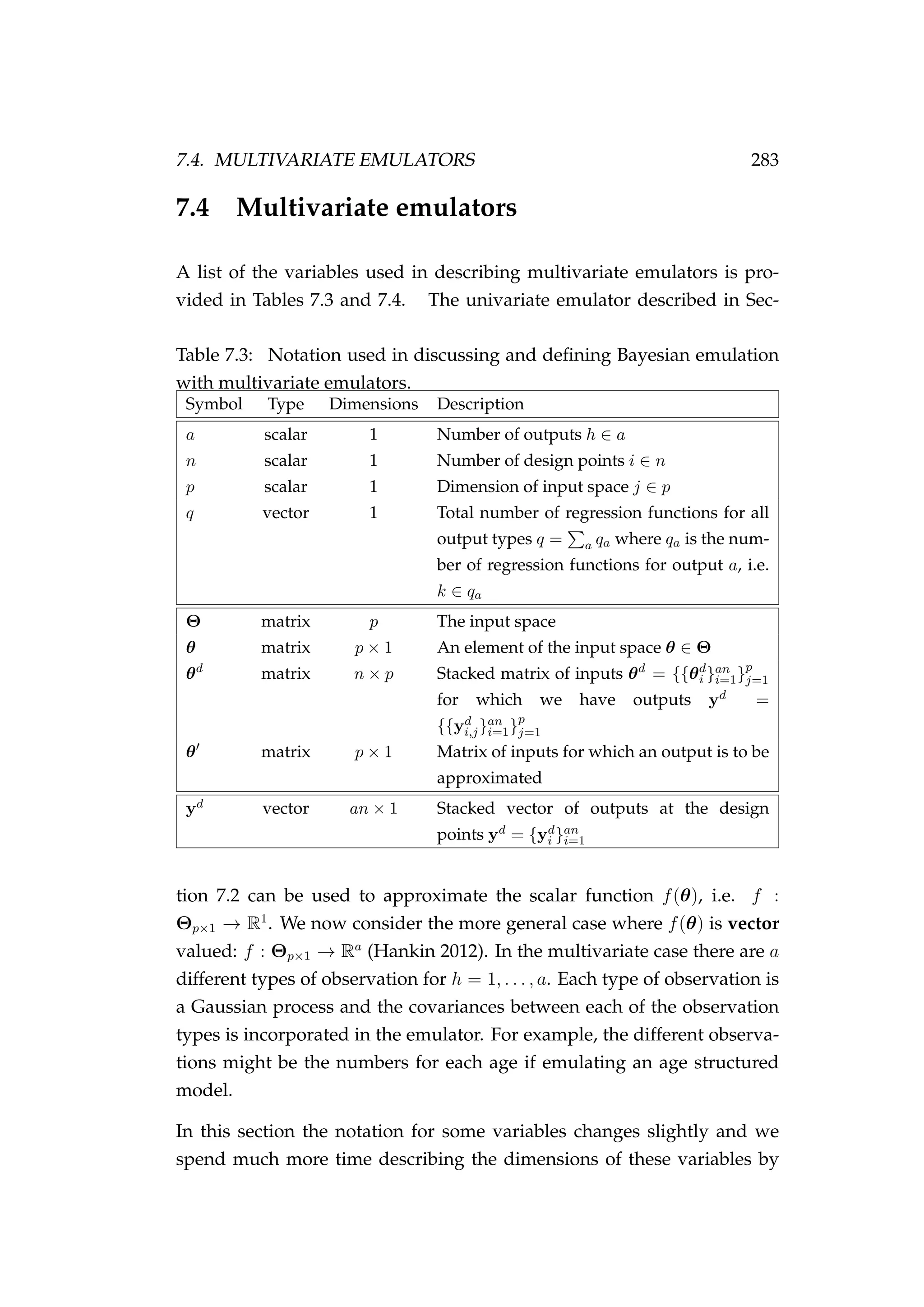
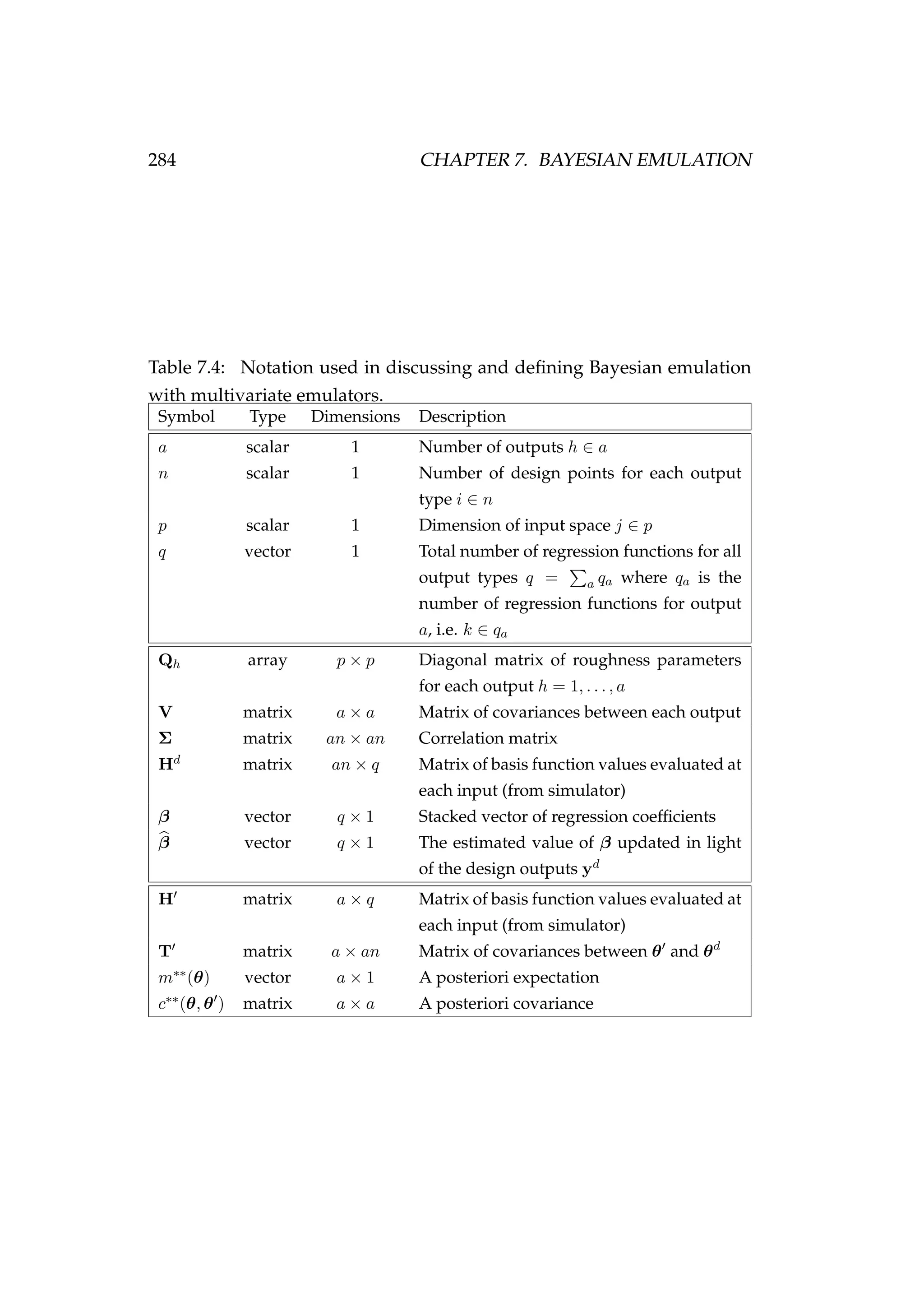
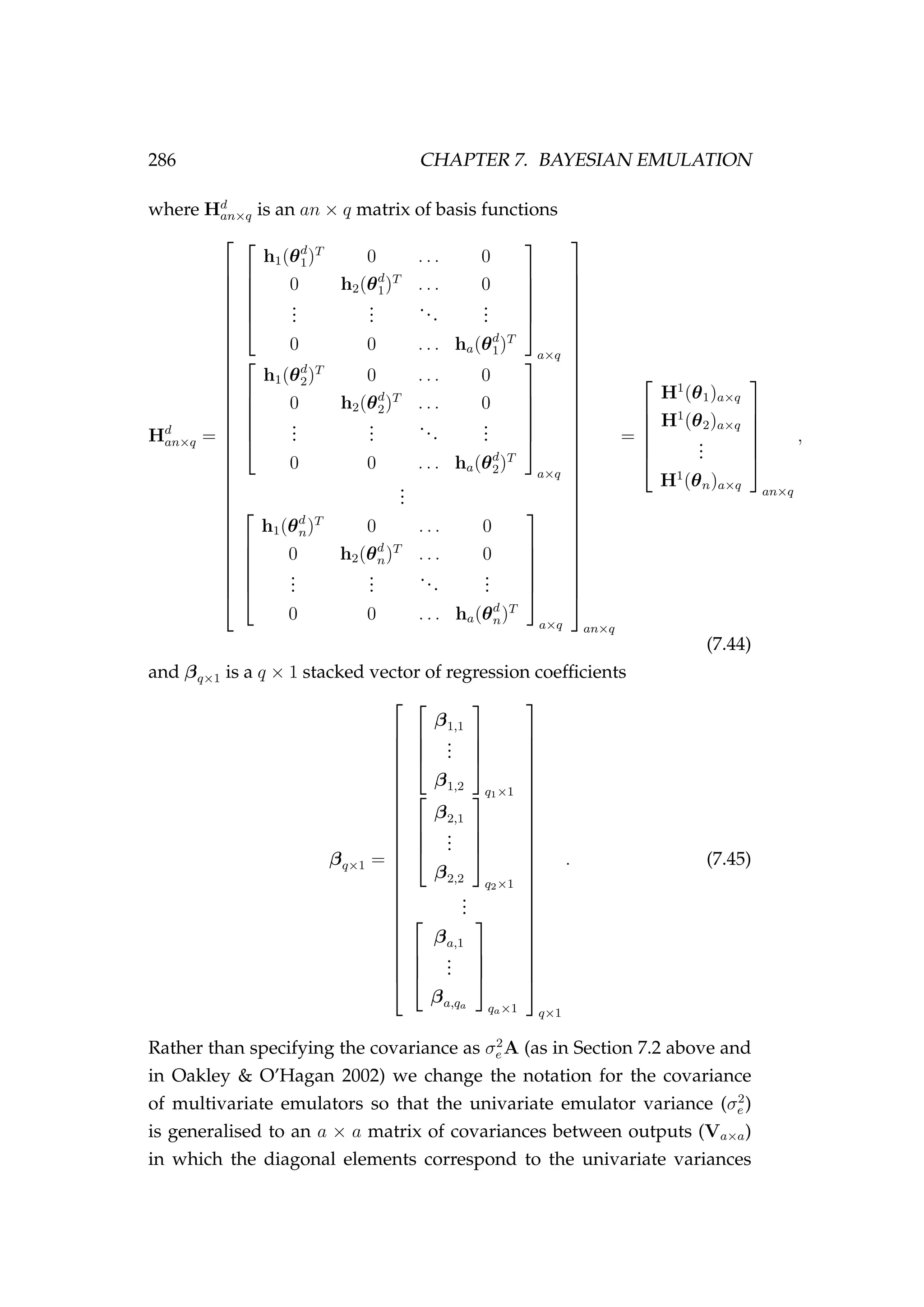
297. 7.4. MULTIVARIATE EMULATORS 285
introducing additional subscripts to make our description of multivariate
emulation as clear as possible. However, they are constructed in much
the same way as univariate emulators so we provide a much less detailed
account of their construction.
As before, we generate a training set known as the design points (θd
i ) and
evaluate our computer model f(θ) relatively few times to generate a set of
outputs (yd
i )
yd
i = f(θd
i ) where i = 1, . . . , n,
yd
an×1 = (yd
1)T
, . . . , (yd
n)T T
, (7.41)
where n is the number of design points. Here yd
i is an a × 1 vector of
outputs for the p × 1 vector of inputs θ.
We then approximate f(θ) by a Gaussian process
ya×1 = fa θ|β, σ2
e , Q ∼ GP (ma×1 (θ|β) , Va×a) ,
E[y]a×1 = E fa θ|β, σ2
e , Q = ma×1 (θ|β) = Ha×qβq×1, (7.42)
conditional on the unknown stacked vector of coefficients β = {βk}q
k=1.
This Gaussian process implies that on the design points our data can be
approximated by
yd
an×1 ∼ N Hd
an×qβq×1, Σan×an (7.43)

298. 286 CHAPTER 7. BAYESIAN EMULATION
where Hd
an×q is an an × q matrix of basis functions
Hd
an×q =





































h1(θd
1)T
0 . . . 0
0 h2(θd
1)T
. . . 0
...
...
...
...
0 0 . . . ha(θd
1)T






a×q





h1(θd
2)T
0 . . . 0
0 h2(θd
2)T
. . . 0
...
...
...
...
0 0 . . . ha(θd
2)T






a×q
...






h1(θd
n)T
0 . . . 0
0 h2(θd
n)T
. . . 0
...
...
...
...
0 0 . . . ha(θd
n)T






a×q































an×q
=






H1
(θ1)a×q
H1
(θ2)a×q
...
H1
(θn)a×q






an×q
,
(7.44)
and βq×1 is a q × 1 stacked vector of regression coefficients
βq×1 =




























β1,1
...
β1,2




q1×1



β2,1
...
β2,2




q2×1
...



βa,1
...
βa,qa




qa×1
























q×1
. (7.45)
Rather than specifying the covariance as σ2
e A (as in Section 7.2 above and
in Oakley & O’Hagan 2002) we change the notation for the covariance
of multivariate emulators so that the univariate emulator variance (σ2
e )
is generalised to an a × a matrix of covariances between outputs (Va×a)
in which the diagonal elements correspond to the univariate variances

299. 7.4. MULTIVARIATE EMULATORS 287
{σ2
e,h}a
h=1. The univariate matrix of roughness scales (Q) is simply repeated
for each output type to {Qh}a
h=1. Thus, the correlation function is
c(θ, θ |Qh)a×a = ch1,h2
i1,i2
=
exp − (θi1 − θi2 )T 1
2
Q−1
h1
+ 1
2
Q−1
h2
−1
(θi1 − θi2 )
1
2
Qh1 + 1
2
Qh2
1
2
Q−1
h1
+ 1
2
Q−1
h2
1
4
,
(7.46)
for h1 = 1, . . . , a, h2 = 1, . . . , a, i1 = 1, . . . , n and i2 = 1, . . . , n, such that
if h1 = h2, then Qh1 = Qh2 , therefore (1
2
Q−1
h1
+ 1
2
Q−1
h2
)−1
= Qh1 = Qh2 and
|(1
2
Qh1 + 1
2
Qh2 )(1
2
Q−1
h1
+ 1
2
Q−1
h2
)|
1
4 = 1, which gives
ch1,h1
i1,i2
= exp − (θi1 − θi2 )T
Q−1
h1
(θi1 − θi2 ) .
This is the same form used in univariate emulators (Equation 7.4,
page 266). The multivariate form basically uses the average roughness
scale when calculating the correlation between two different output pa-
rameters. It then follows that the covariance matrix is
Σan×an = Vh1,h2 ch1,h2
i1,i2
, (7.47)
or more explicitly

300. Σan×an =



































Va×a






c1,1
1,1 c1,2
1,1 . . . c1,a
1,1
c2,1
1,1 c2,2
1,1 . . . c2,a
1,1
...
...
...
...
ca,1
1,1 ca,2
1,1 . . . ca,a
1,1






a×a
Va×a






c1,1
1,2 c1,2
1,2 . . . c1,a
1,2
c2,1
1,2 c1,2
1,2 . . . c2,a
1,2
...
...
...
...
ca,1
1,2 ca,2
1,2 . . . ca,a
1,2






a×a
. . . Va×a






c1,1
1,n c1,2
1,n . . . c1,a
1,n
c1,1
1,n c1,2
1,n . . . c2,a
1,n
...
...
...
...
ca,1
1,n ca,2
1,n . . . ca,a
1,n






a×a
Va×a






c1,1
2,1 c1,2
2,1 . . . c1,a
2,1
c2,1
2,1 c2,2
2,1 . . . c2,a
2,1
...
...
...
...
ca,1
2,1 ca,2
2,1 . . . ca,a
2,1






a×a
Va×a






c1,1
2,2 c1,2
2,2 . . . c1,a
2,2
c1,2
2,2 c2,2
2,2 . . . c2,a
2,2
...
...
...
...
c1,a
2,2 c2,a
2,2 . . . ca,a
2,2






a×a
. . . Va×a






c1,1
2,n c1,2
2,n . . . c1,a
2,n
c1,2
2,n c2,2
2,n . . . c2,a
2,n
...
...
...
...
c1,a
2,n c2,a
2,n . . . ca,a
2,n






a×a
...
...
...
...
Va×a






c1,1
n,1 c1,2
n,1 . . . c1,a
n,1
c1,2
n,1 c2,2
n,1 . . . c2,a
n,1
...
...
...
...
c1,a
n,1 c2,a
n,1 . . . ca,a
n,1






a×a
Va×a






c1,1
n,2 c1,2
n,2 . . . c1,a
n,2
c1,2
n,2 c2,2
n,2 . . . c2,a
n,2
...
...
...
...
c1,a
n,2 c2,a
n,2 . . . ca,a
n,2






a×a
. . . Va×a






c1,1
n,n c1,2
n,n . . . c1,a
n,n
c1,2
n,n c2,2
n,n . . . c2,a
n,n
...
...
...
...
c1,a
n,n c2,a
n,n . . . ca,a
n,n






a×a



































an×an
,
(7.48)
where indicates element-wise multiplication.

301. 7.4. MULTIVARIATE EMULATORS 289
We then calibrate our approximation by finding the REML estimate of β
βγ|θd
, yd
, Q, D1
= (Hd
an×q)T
(Σ−1
γ )an×anHd
an×q
−1
(Hd
an×q)T
(Σ−1
γ )an×anyd
an×1,
(7.49)
where
Σγ = Σan×an + Dan×an,
Dan×an = diag D1
a×a, . . . , D1
a×a ,
D1
a×a = diag σ2
γ,1, . . . , σ2
γ,a ,
where (σ2
γ,1, . . . , σ2
γ,a) must be estimated. Similar to Hankin (2012), we
choose to to this independently for each output type a and so the methods
used in Section 7.3 (page 278) above can be used. However, this is an area
that requires further research. Future choices here include: further gener-
alisation so that D1
is a full a × a matrix (rather than a diagonal matrix),
or; further simplification (if all σ2
γ’s are assumed constant) to D1
= σ2
γI.
Given βγ, Σγ and D1
, we proceed with the construction of a multivariate
emulator that incorporates REML estimation. We construct the approxi-
mation
y = fu θ|β, Σ, θd
, yd
, Q ∼ GP m∗
a×1 θ|β, θd
, yd
, Q , c∗
a×a θ, θ |θd
, Q ,
(7.50)
where
m∗
a×1 θ|β, θd
, yd
, Q = (H1
)T
a×qβq×1 + TT
a×anΣ−1
an×an yd
an×1 − Hd
an×qβq×1 ,
(7.51)
c∗
a×a θ, θ |θd
, Q = c θa×p, θa×p|Qa a×a
− (Ta×an)T
Σ−1
an×anTa×an,
(7.52)
Ta×an = c θa×p|θd
an×p, Qa a×a
, . . . , c θa×p|θd
an×p, Qa a×a a×an
.
(7.53)
Finally, we construct the emulator
ya×1 = fc θ|β, Σγ, θd
, yd
, Q ∼ GP m∗∗
a×1 θ|β, θd
, yd
, Q , (Σγ)an×an ,
(7.54)

302. 290 CHAPTER 7. BAYESIAN EMULATION
where
m∗∗
a×1 θ|β, θd
, yd
, Q = H1
a×q(βγ)q×1
+ Ta×an(Σ−1
γ )an×an yd
an×1 − Hd
an×q(βγ)q×1
an×1
,
(7.55)
c∗∗
a×a θ, θ |θd
, Q = c∗
a×a θa×p, θa×p|θd
an×p, Qa
+ H1
a×q − Ta×an(Σ−1
γ )an×anHd
an×q
× (Hd
)T
an×q(Σ−1
γ )an×anHd
an×q
−1
× H1
a×q − Ta×an(Σ−1
γ )an×anHd
an×q
T
, (7.56)
and H1
a×q is an a × q matrix of basis functions
H1
a×q =






h1(θ )T
0 · · · 0
0 h2(θ )T
0
...
...
...
...
0 0 · · · ha(θ )T






a×q
,
where hj(θ(j)
)T
are the basis functions for the output types j = 1, . . . , p.
7.5 Inference on an emulator
The purpose of a Bayesian emulator is to make inference of computation-
ally expensive models tractable. That is, a good emulator should provide
an unbiased and relatively precise approximation of a computationally ex-
pensive model, yet be much faster to evaluate, allowing the use of stan-
dard inference procedures such as MCMC (e.g. Henderson et al. 2009).
Once an emulator of a computationally expensive model has been devel-
oped and conditioned, the emulator simply replaces the original model
when making inference about the system.
We now describe the relationship between the physical system, the sim-
ulator (i.e. the computationally expensive model) and the emulator. We
denote observations of the system as the vector yo
. We denote the true

303. 7.5. INFERENCE ON AN EMULATOR 291
physical system values as the vector y∗
. We describe the relationship be-
tween the observations yo
and and the true value y∗
as
yo
= y∗
+ εo
, (7.57)
where εo
is the observation error. Assuming that the simulator is a sequen-
tial evolving system (e.g. a state-space biomass dynamics model) then the
relationship between the simulator and the system is then expressed as
y∗
= f(θ) + εp
, (7.58)
where εp
is the process error of the model (if we are not considering a
sequential evolving system then we simply ignore this step). A belief net-
work for standard inference is
f(·) f(θ) y yo
θ εp
εo
We now consider how this belief network looks if we introduce a Bayesian
emulator with a conditioned approximating function fc(·) (which has
mean and variance m∗∗
(·) and σ2
e c∗∗
(·, ·) respectively). Because fc(·) is as-
sumed to be a close approximation of f(·), a belief network for inference
on an emulator is
f(·) f(θ) fc θ|θd
, yd
, Q y yo
θ θ, θd
, yd
, Q εp
εo
Given that we observe data yo
, using Bayes’ theorem we can write
p(θ|yo
) =
p(yo
|θ)p(θ)
p(yo)
∝ p(yo
|θ)p(θ), (7.59)
where p(θ) is the prior distribution of the parameter(s) before any data is
observed, p(yo
|θ) is the sampling distribution of the observed data con-
ditional on its parameters (also termed the likelihood L(θ; yo
) = p(yo
|θ)),
p(yo
) is the marginal likelihood and p(θ|yo
) is the posterior distribution of
the parameters conditional on the observed data yo
. Under the emulator
we write
p(θ|yo
) = p θ|yo
, yd
, θd
, Q ∝ p yo
|θ yd
, θd
, Q p(θ), (7.60)

304. 292 CHAPTER 7. BAYESIAN EMULATION
where the emulator itself defines the likelihood
p (yo
|θ) = p yo
|θ yd
, θd
, Q ∼ N m∗∗
θ|θd
, yd
, Q , σ2
e c∗∗
θ, θ |θd
, Q .
(7.61)
Now we can introduce observational errors σ2
o (iid)
y|θ, σ2
o β, σ2
e , yd
, θd
, Q ∼ N m∗∗
θ|β, θd
, yd
, Q , σ2
o + σ2
e θd
, yd
, Q c∗∗
θ, θ |θd
, Q ,
(7.62)
and finally we can proceed using standard methods
p(θ, σ2
o|yo
) ∝ p(yo
|θ, σ2
o)p(θ)p(σ2
o)
∝ p(yo
, y|θ, σ2
o)p(θ)p(σ2
o)dy
∝ p(yo
|y, σ2
o)p(y|θ, σ2
o)p(θ)p(σ2
o)dy
approx. ∝ p(yo
|y, σ2
o)p∗∗
(y|θ, yd
, θd
, Q)p(θ)p(σ2
o)dy, (7.63)
identifying the emulator as p∗∗
(y|θ, yd
, θd
, Q).
7.6 Univariate emulation of a biomass dynamics
model
This example develops a univariate emulator of a biomass dynamics
model and uses this emulator, nested inside a state-space framework, to
make inference about a simulated data set.
7.6.1 The simulator
We begin with a biomass dynamics simulation model. As in Chapter 5
(page 137), we use the state-space version of this model
J1 = K,
Jt = Jt−1 + rJt−1 (1 − Jt−1) −
Ct−1
K
eεp
t 2 ≤ t ≤ T, (7.64)
It = qKJteεo
t ∀t, (7.65)

305. 7.6. UNIVARIATE EMULATION OF A BIOMASS DYNAMICS MODEL293
where
εp
t
iid
∼ N(0, σ2
p) and εo
t
iid
∼ N(0, σ2
o).
Here Jt = Bt/K where Bt is the biomass (tonnes) at the beginning of time
t, r is the intrinsic rate of population increase, K is the carrying capacity
(tonnes), and Ct is the catch (tonnes) at time t. εo
t and εp
t are iid observation
and process deviations at time t with variances σ2
o and σ2
p. The hidden
Markov of this model can be represented as:
J1 J2 · · · Jt · · · JT
I1 I2 It IT
C1 Ct−1 CT−1
σ2
p σ2
p σ2
p σ2
p σ2
p
σ2
o σ2
o σ2
o σ2
o
Similar to the packhorse rock lobster simulations in Chapter 5, we simu-
late CPUE (It) and biomass (Bt) from this model using the parameter set
outlined in Table 7.5 and the catch history used in the packhorse rock lob-
ster simulations (Section 5.3.2, page 141).
Table 7.5: Parameter values used in the biomass dynamics
model simulation.
Parameter Value Units Description
r 0.17 tonnes−1 Intrinsic rate of population in-
crease
K 1500 tonnes Carrying capacity
q 0.002 tonnes−1 Catchability coefficient
σo 0.5 - Observation error standard devi-
ation
σp 0.001 tonnes Process error standard deviation

306. 294 CHAPTER 7. BAYESIAN EMULATION
7.6.2 The emulator
Our goal is to construct a univariate emulator of the process component
of the simulation model (Equation 7.64) and do inference on the emu-
lator coupled with the observation component (Equation 7.65). To do
this, we replace the process equation that defines each latent state in
our model with a conditioned univariate emulator, i.e. Jt = f(θt) is re-
placed by Jt = fc(θt) where E[Jt] = m∗∗
(θt) and the emulator inputs are
θt = (Jt−1, r, K, Ct−1).
Emulator inputs (θt)
We use a Latin hypercube design to produce n = 100 input vectors (θd
=
{θd
i }n
i=1) within realistic ranges for each of the emulated model parameters
(Figure 7.5). We then use Equation 7.64 to obtain the design points yd
=
{yd
i }n
i=1.
Emulator outputs (yt)
The basis function used was h(θ)T
= (1, Jt−1, r, K, Ct−1). Roughness
lengths (Q) were estimated and fixed a priori. The emulator was condi-
tioned on the design inputs (θd
) and outputs (yd
) of the simulator.
We test the performance of the emulator by drawing another 100 input
parameters (θ) from the parameter space (Θ), running the model another
100 times using each of these parameter sets to obtain outputs (y), but not
using these inputs/outputs to condition the emulator. Instead we provide
these inputs to the already conditioned emulator and obtain the emulated
outputs also to test the performance of the emulator. The biomass pre-
dicted by the emulator was very close to the biomass derived using Equa-
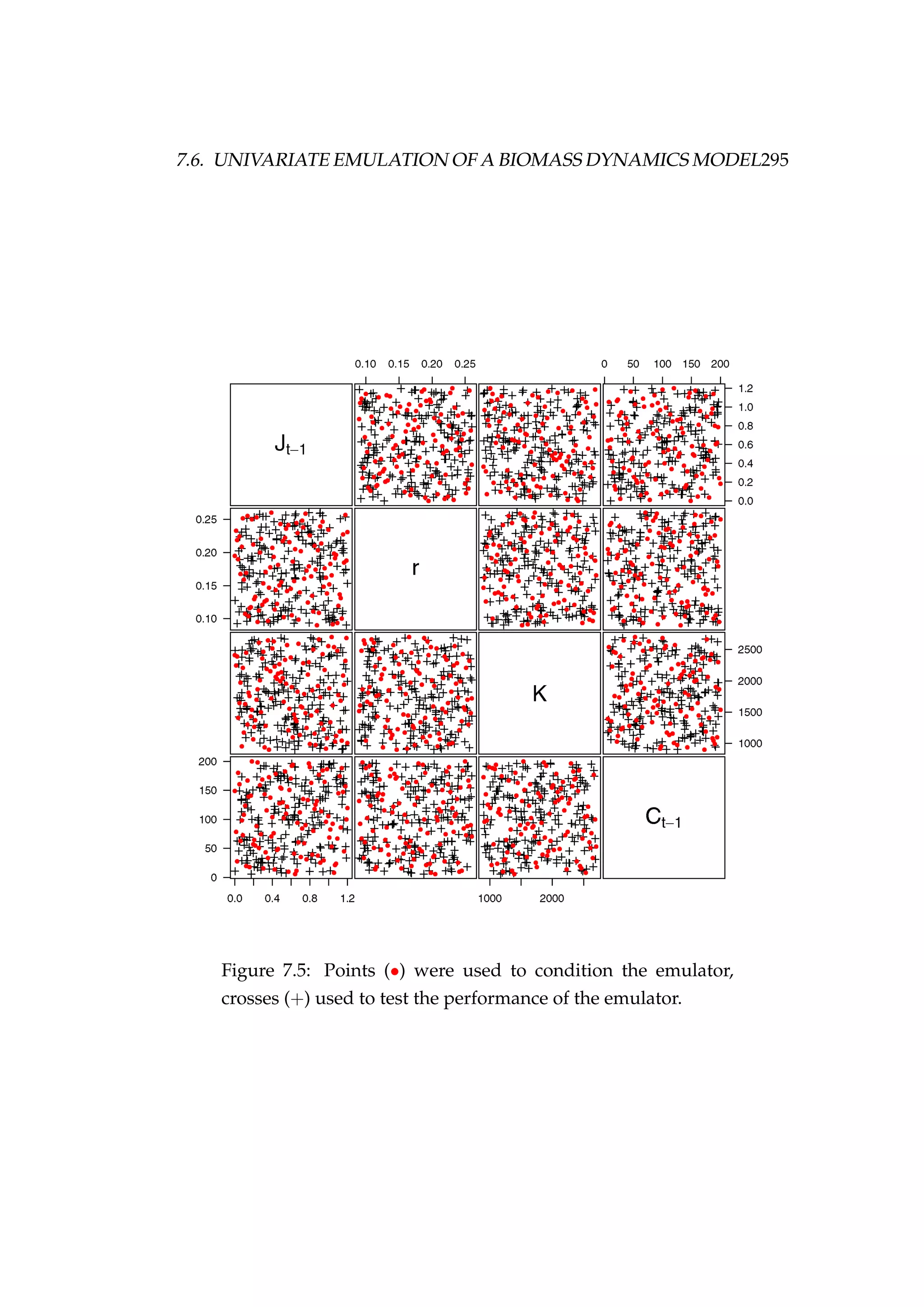
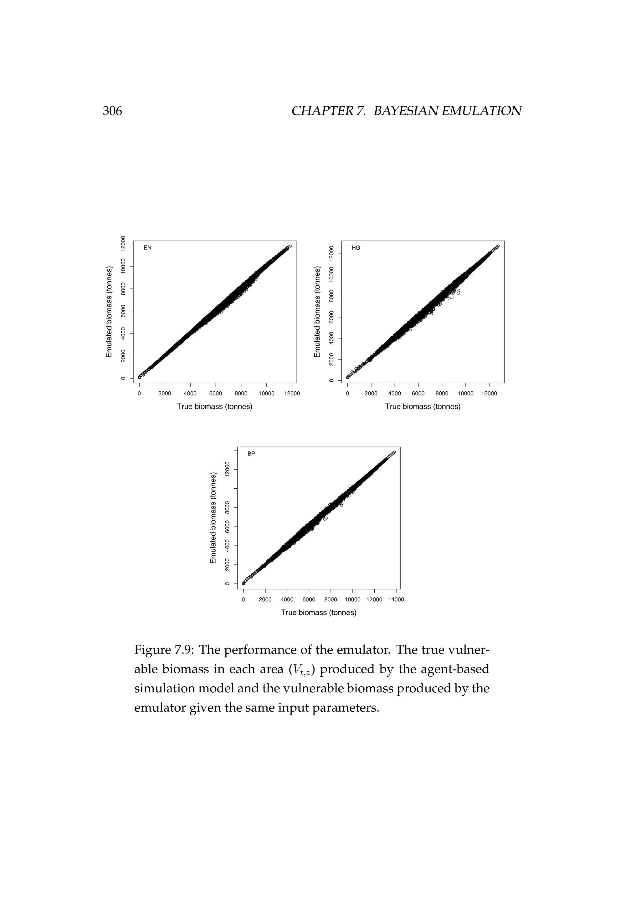
tion 7.64, given the same input parameters and covariates (Figure 7.6).

307. 7.6. UNIVARIATE EMULATION OF A BIOMASS DYNAMICS MODEL295
Figure 7.5: Points (•) were used to condition the emulator,
crosses (+) used to test the performance of the emulator.

308. 296 CHAPTER 7. BAYESIAN EMULATION
Figure 7.6: Simulated biomass versus the emulated biomass
[left] and residual [right].
7.6.3 Inference
We are interested the probabilistic relationship between the following:
• The data y: the catch per unit effort (It). Let y = {It}T
t=1
• The covariates z: the catch (Ct). Let z = {Ct}T
t=1
• The unknown process parameters ψ: the intrinsic rate of popula-
tion increase (r), the carrying capacity of the population (K) and the
process error variance (σ2
p). Let ψ = {r, K, σ2
p}
• The unknown observation parameters φ: the catchability coefficient
(q) and the observation error variance (σ2
o). Let φ = {q, σ2
o}
• The unknown latent states x: the depletion (Jt). Let x = {Jt}T
t=1
Using Bayes’ theorem, the posterior distribution of the model parameters
(ψ and φ) and the states (x), given the data (y) and covariates (z) is
π(ψ, φ, x|y, z) ∝ π(ψ, φ, x|z)π(y|ψ, φ, x), (7.66)

309. 7.6. UNIVARIATE EMULATION OF A BIOMASS DYNAMICS MODEL297
where
π (ψ, φ, x|z) = π r, K, q, σ2
o, σ2
p, x|z
= π(r)π(K)π(q)π(σ2
o)π(σ2
p)π x|z, r, K, σ2
p
= π(r)π(K)π(q)π(σ2
o)π(σ2
p)π J1|K, σ2
p
T
t=2
π Jt|Jt−1, Ct−1, r, K, σ2
p ,
π (y|x, ψ, φ) = π y|x, K, q, σ2
o =
T
t=1
π It|Jt, K, q, σ2
o . (7.67)
Here the component T
t=2 π Jt|Jt−1, Ct−1, r, K, σ2
p is evaluated by the em-
ulator and we state
Jt|θ, β, σ2
e , θd
, yd
, Q ∼ N m∗∗
θ|β, θd
, yd
, Q , σ2
e c∗∗
θ, θ |θd
, Q ,
(7.68)
where θ is a vector of emulator inputs (i.e. a collection of parameters,
latent states and covariates). Here the emulator is constructed using the
inputs θ = {Jt−1, Ct−1, r, K}. Notice that the observation parameters (φ)
are not required by the emulator. We also exclude the process error vari-
ance (σ2
p) from the emulator and model process error within the state-space
framework. It would be more common for the stochastic computer model
to provide outputs after process error is applied (i.e. if we are thinking
about complex computationally expensive computer models). Although
we do not incorporate the process error in the emulator in this example, it
is implicitly included in the next example. Here we embed the emulator
within a state-space biomass dynamics model replacing the core (i.e. the
process equation) with the conditioned emulator
Jt|θt−1, σ2
p = fc θ|β, σ2
e , θd
, yd
, Q eεp
t , (7.69)
It|Jt, φ = qKJteεo
t = qBteεo
t , (7.70)
noticing that the observation equation is only conditional on Jt and φ.
Now standard inference procedures may be applied to the emulator to
obtain best input parameters (θ) and observation parameters (φ) for our
simulator conditional on the observations of the system. We specify rea-
sonably informative log-normal priors for the parameters r and K (see
Figure 7.7 below), and high variance inverse gamma distributions for the

310. 298 CHAPTER 7. BAYESIAN EMULATION
parameters q, σ2
o and σ2
p (i.e. IG(0.001, 0.001)). We run an MCMC of 1 mil-
lion iterations, saving every 1000th sample, to obtain 1000 samples from
the posterior distribution.
We only report the MCMC trace plots and posterior densities (Figure 7.7),
but note that the model fit to the CPUE data and the biomass trajec-
tory arising from this fit provide an excellent match to the simulated
CPUE/biomass. MCMC did an excellent job of recovering most of the
parameter values specified in the simulation, as we would expect given
that the performance of the Bayesian emulator (Figure 7.6). As we also
found in Chapter 5 (page 129), the observation and process error variance
parameters were slightly under and overestimated, respectively. This is to
be expected given the reasonably high observation error specified in the
simulation (see Table 7.5).
7.7 Multivariate emulation of a stochastic agent-
based model
Finally we describe a stochastic multivariate Bayesian emulator for the
agent-based snapper model described in Chapter 4 (page 89). The ABM
is a spatially explicit multi-generational agent-structured fish simulation
model. The parameter values used in the simulation and structural as-
pects of the ABM were cherry picked from Francis & McKenzie (2013), and
older versions of this stock assessment. Because the ABM used here sim-
plified some aspects of the SNA 1 stock assessment and includes untested
hypothesis about the dynamics of these stocks, none of the work in this
chapter should be used to make inference about the SNA 1 fish stocks.
This work is intended as a proof of concept only.
7.7.1 The simulator
A spatially explicit ABM of snapper in northern New Zealand (SNA 1) was
developed using the agent-based simulation model discussed in Chapter 4

311. 7.7. MULTIVARIATE EMULATION OF A STOCHASTIC AGENT-BASED MODEL299
Figure 7.7: MCMC trace plots and posterior densities sam-
pled from the state-space biomass dynamics Bayesian emula-
tor. Posterior traces and densities are indicated as black lines,
priors as dashed black lines (the priors for the catchability co-
efficient q, the observation error, and the process error are all
uninformative inverse gamma priors so are omitted from the
plot), and values specified in simulation as solid blue lines.

312. 300 CHAPTER 7. BAYESIAN EMULATION
(page 89). Background information on this species can be found in Chap-
ter 3 (page 77).
The ABM was developed to capture the hypothetical life cycle of snapper
in SNA 1. The model was constructed as a three-stock (j), three-area (z),
two sex (s) model (with the same demographic parameters for each sex,
i.e. really a single sex model) with fifty age groups (a = 1, . . . , 50+). The
spawning stock biomass (SSBt) is defined as the mature biomass of both
females and males. The three areas in the model are labelled: East North-
land (EN), the Hauraki Gulf (HG) and the Bay of Plenty (BP). Immature
fish are distributed in each of the three areas. Each year (t) the fish move
about each of the three model areas with probability based on a fixed mi-
gration matrix
Ω =



0.77 0.05 0.18
0.09 0.51 0.40
0.24 0.28 0.48


 .
Each agent’s (i) home (h) is defined as the area that they recruited to in
the model. Mature fish return home to spawn. The fish in each area at the
time spawning stock biomass is calculated make up the stock in that area.
Thus there were two migration events per year in the model.
The model was initialised with an equilibrium age and spatial distribu-
tion structure. In the model, the initial equilibrium state was found itera-
tively in two phases. The first phase involved applying recruitment, natu-
ral mortality and ageing processes. Movement was not permitted during
this phase. In the second phase, movement processes were introduced.
The duration of each phase of initialisation was 100 years. The length of
these two phases was determined by running the model a few times and
checking that population biomass in each area reached a plateau and re-
mained there for at least a couple of decades and that the age-structure of
the population looked realistic (i.e. the numbers at age roughly showed
an exponential decline).
Following initialisation, the model was run over a period of 114 years,
from 1900 to 2013. During this period, fishing mortality and tagging pro-
cesses consistent with actual catches and tagging in the history of the SNA

313. 7.7. MULTIVARIATE EMULATION OF A STOCHASTIC AGENT-BASED MODEL301
1 fishery were applied. The parameter values specified in the simulation
model are provided below in Table 7.6. Initial exploration showed that
Table 7.6: The key parameter values used in specifying the
agent based snapper (SNA 1) simulation model. For a more
detailed list of the parameter used in this simulation see Ap-
pendix D (page 351).
Attribute Parameter Value
Length L∞ 58.8
k 0.102
t0 -1.11
σL∞ 0.01
σk 0.001
cv∆ 0.001
Length-weight α 4.467e-08
β 2.793
σα 1e-10
σβ 0.001
Maturity A50 4
Ato95 4.7
L 3
R 5
σA50 0.001
σAto95 0.001
Natural mortality M 0.075
σM 0.001
Selectivity γ1 6.05
γL 2.31
γR 100
Recruitment R0 443493, 950050, 318619
h 0.85
σR 0.14
ρ 0.6
the actual R0 estimated in the 2013 SNA 1 stock assessment could not be
used because the model consumed all of the computer’s primary memory

314. 302 CHAPTER 7. BAYESIAN EMULATION
(RAM) (i.e. it resulted in too many agents being created). To avoid this, we
tried specifying a model with more fish per agent. But, because agents are
allowed to split (see Chapter 4, page 102) and we wanted to avoid merging
too many agents as this tends to results in the dilution of agent attributes
(see the see Chapter 4, page 106 for more detail), the number of agents cre-
ated was still too great and resulted in the model exceeding the computers
memory. Instead, the smaller R0 parameters identified in Table 7.6 were
used and the catches scaled down accordingly. The actual input file for
the simulation and plots illustrating a selection of the model dynamics are
included in Appendix D (page 351).
The ABM has the ability to introduce stochasticity in almost all modelled
processes (e.g. growth, length-weight relationship, natural mortality). In
this example we did not turn stochasticity off, but instead specified rela-
tively small standard deviation parameters for all stochastic processes (see
Table 7.6 and Appendix D, page 351). We proceeded in this way so that we
can better test the performance of Bayesian emulation in capturing some
of the complexity inherent in this model, rather than testing how well the
method copes in the face of uncertainty. However, this would be an inter-
esting avenue for further research.
7.7.2 The emulator
Ideally we would construct and condition a Bayesian emulator that takes
all of the numbers at age in a single time-step, key model parameters,
and the the catch as inputs (i.e. θt = {Na,t,z, Ct,z, R0,z, . . .}) and pro-
vides the numbers at age in the following time-step as the output (i.e.
yt+1 = {Na,t+1}). A series of emulators could then be linked together to
form the process model of the numbers at age in the population.
However, initial exploration and attempts to emulate the numbers at age
in this way proved difficult because emulators performed poorly and were
too slow to be of any use (in MCMC). Instead we decided to wrap most
of the complexity of the ABM into a stochastic multivariate emulator that
models the evolution of the vulnerable biomass (Vt,z) of fish by area (z)

315. 7.7. MULTIVARIATE EMULATION OF A STOCHASTIC AGENT-BASED MODEL303
and time (t). This system can be represented graphically as:
V1 · · · Vt−1 Vt Vt+1 · · · VT
I1 It−1 It It+1 IT
C1 Ct−1 Ct Ct+1 CT
where Vt, Ct and It are vectors of the vulnerable biomass, the catch and
the CPUE by area, respectively.
We provide further discussion on age-structured Bayesian emulators in
the discussion at the end of this chapter (section 7.8, page 310).
Emulator inputs (θt)
We choose a subset of the models key parameters (Table 7.6) to estimate
and fix the remaining parameters. The parameters that we chose to em-
ulate include each stocks average recruitment (R0,z), the peak (γ1) and
left hand limb (γL) of the double normal selectivity curve, the catchabil-
ity coefficient (q), the recruitment standard deviation (σR) and the CPUE
observation error standard deviation (σo). These parameters, along with
the catch at any given time-step (Ct,z) and the vulnerable biomass in any
given time-step (Vt,z), will be the inputs for our Bayesian emulator (i.e.
θt = {Vt,z, Ct,z, R0,z, γ1, γL, q, σR, σo}).
The input design, on which the emulator is conditioned, is constructed
with n = 1000 sets of parameters drawn using the Latin hypercube design
within sensible bounds (Figure 7.8).
We then run the ABM 1000 times, using these 1000 sets of input parame-
ters (θd
). The the inputs and outputs (yd
) of these 1000 runs we compiled
into a single matrix of inputs and a single matrix of linked outputs. Be-
cause the ABM is simulating a fishery over 114 years, and the emulator
only emulates a single year at a time, we really have 1000 sets of inputs
that relate to 1000 × 114 sets of outputs. As an input design of this di-

316. 304 CHAPTER 7. BAYESIAN EMULATION
Figure 7.8: The input design (θd
) for each key parameter that
was used to condition the emulator [+] and the true parameter
values that were specified in the agent-based simulation model
[•].

317. 7.7. MULTIVARIATE EMULATION OF A STOCHASTIC AGENT-BASED MODEL305
mension is far to big for use in Bayesian emulation (and probably too big
for any computer to handle, I tried inverting this matrix by mistake and
crashed my computer), we reduced the dimensionality of the input design
by selecting a single output year at random to pair with each input, thus
we are back to having and input design of n = 1000.
Emulator outputs (yt)
The multivariate emulator is conditioned to return the vulnerable biomass
in the following time-step as its output (i.e. yt = {Vt,z}). We test the per-
formance of the emulator by drawing another 1000 input parameters (θ)
from the parameter space (Θ), running the ABM another 1000 times using
each of these parameter sets to obtain outputs (y), but not using these in-
puts/outputs to condition the emulator. Instead we provide these inputs
to the already conditioned emulator and obtain the emulated outputs also
(Figure 7.9).
7.7.3 Inference
We are interested the probabilistic relationship between the following:
• The data y: the catch per unit effort by area (It,z). Let y =
{{It,z}T
t=1}Z
z=1
• The covariates z: the catch by area (Ct,z). Let z = {{Ct,z}T
t=1}Z
z=1
• The unknown process parameters ψ: the virgin recruitment by area
(R0,z), the selectivity parameters (γ1 and γL), and the recruitment
variance (σ2
R). Let ψ = {{R0,z}Z
z=1, γ1, γL, σ2
R}
• The unknown observation parameters φ: the catchability coefficient
(q) and the observation error variance (σ2
o). Let φ = {q, σ2
o}
• The unknown latent states x: the vulnerable biomass (tonnes) in
each area (Vt,z). Let x = {{Vt,z}T
t=1}Z
z=1

318. 306 CHAPTER 7. BAYESIAN EMULATION
Figure 7.9: The performance of the emulator. The true vulner-
able biomass in each area (Vt,z) produced by the agent-based
simulation model and the vulnerable biomass produced by the
emulator given the same input parameters.

319. 7.7. MULTIVARIATE EMULATION OF A STOCHASTIC AGENT-BASED MODEL307
Using Bayes theorem, the posterior distribution of the model parameters
(ψ and φ) and the states (x), given the data (y) and covariates (z) is
π(ψ, φ, x|y, z) ∝ π(ψ, φ, x|z)π(y|x, φ), (7.71)
where
π (ψ, φ, x|z) = π R0,z, q, γ50, γ95, σ2
o, σ2
R, x|z
= π(R0,z)π(q)π(γ50)π(γ95)π(σ2
o)π(σ2
R)π x|z, R0, γ50, γ95, σ2
R
= π(R0,z)π(q)π(γ50)π(γ95)π(σ2
o)π(σ2
R)π(V1,z)
×
T
t=2
Z
z=1
π Vt,z|Vt−1,z, Ct−1,z, R0,z, γ50, γ95, σ2
R
π (y|x, φ) = π y|x, q, σ2
o =
T
t=1
Z
z=1
π It,z|Vt,z, q, σ2
o . (7.72)
The component π (x|z, R0, γ50, γ95, σ2
R) is the ABM, and is computationally
expensive, taking several hours to do a single evaluation, making stan-
dard inference impractical. Instead, we condition a multivariate Bayesian
emulator to this evolution equation
Vt,z|θ, β, σ2
e , θd
, yd
, Q ∼ N m∗∗
θ |β, θd
, yd
, Q, V , σ2
e c∗∗
θ, θ |θd
, Q ,
(7.73)
where θ is a vector of emulator inputs (i.e. a collection of parameters,
latent states and covariates). Here the emulator is constructed using the
inputs θ = {Vt−1,z, Ct−1,z, R0,z, γ50, γ95, σ2
R}. The likelihood of this model
is made up of two main components: the likelihood of the CPUE obser-
vations (It) and the likelihood of the vulnerable biomass (tonnes) latent
states (Vt,z). The likelihood of the CPUE observations is
log (It,z) |Vt,z, q, σ2
o, ω, ∼ N log (qVt,z) , σ2
o . (7.74)
The two main components of the likelihood can be split into even smaller
subcomponents made up of just single areas z and years t. When a param-
eter or latent state is proposed within MCMC, then only those subcom-
ponents relevant to the proposal need be evaluated. Each of the MCMC
proposals and the subcomponents of the likelihood that need to be evalu-
ated are as follows:

320. 308 CHAPTER 7. BAYESIAN EMULATION
• When proposing R∗
0,z, γ∗
50, γ∗
95 or σ2∗
R evaluate
log (Vt,z) ∼ N log (µt,z) , σ2
e c∗∗
(·) 2 ≤ t ≤ T, ∀z.
• When proposing q∗
or σ2∗
o evaluate
log (It,z) ∼ N log (qVt,z) , σ2
o ∀t, ∀z.
• When proposing V ∗
t,z evaluate
log (It,z) ∼ N log qV ∗
t,z , σ2
o ,
log V ∗
t,z ∼ N log (µt,z) , σ2
e c∗∗
(·) ∀z,
log (Vt+1,z) ∼ N log (µt+1,z) , σ2
e c∗∗
(·) ∀z.
Early exploration suggested that MCMC was not mixing well. We there-
fore specified highly informative log-normal prior distributions for all
model parameters in an attempt to improve mixing (see Figure 7.10 for
plots of these priors). Despite running a long MCMC chain of 3 million
iterations, taking roughly one week to complete (saving every 1000th it-
eration to yield 3000 samples from the posterior distribution), the MCMC
chains still did not mix well (Figure 7.10). The lack of mixing was most
pronounced in the catchability coefficient (q). Despite the poor mixing
of the key parameters, the log-likelihoods and log-priors appeared to be
mixing well (Figure 7.11). The fit to the CPUE data was also excellent (Fig-
ure 7.12) and the posterior distribution of the vulnerable biomass in each
area matched closely with the simulated vulnerable biomass (Figure 7.13).
However, given the highly informative priors placed on the key parame-
ters, this is not surprising. We therefore conclude that Bayesian emulation
did not work very well in this example. The root of the problem is its
speed, or rather lack of. Despite simplifying the problem considerably by
reducing the number of parameters to be emulated to the bare minimum,
the emulator was still relatively slow, resulting in a slow MCMC sampler.
We consider that an MCMC that takes longer than a week, and does not
result in adequately mixed MCMCs, is beyond practical application.

321. 7.7. MULTIVARIATE EMULATION OF A STOCHASTIC AGENT-BASED MODEL309
Figure 7.10: MCMC trace plots [left column] and posterior den-
sities [right column] for each of the emulated key model pa-
rameters.

322. 310 CHAPTER 7. BAYESIAN EMULATION
Figure 7.11: MCMC trace plots [left column] and posterior
densities [right column] log-likelihood of the CPUE, the log-
likelihood of the vulnerable biomass state and the log-prior.
Although the method has fallen short in this example, we have developed
a proof of concept for the method, and further developed the method it-
self. We hope that these beginnings will stimulate further research into
Bayesian emulation, in fisheries science or otherwise. We discuss some
good starting points for future research below.
7.8 Discussion
This chapter synthesised aspects from all of the preceding chapters of this
thesis. Snapper (Chapter 3, page 77) was used as case study species and
an agent-based model was developed based broadly on the dynamics of
the species in SNA 1 (Chapter 4, page 89). Bayesian emulation (first intro-
duced in Chapter 2, page 71) is covered in more detail, the methods are
extended beyond the scope of the current literature, and the methods are
applied to fisheries specific problems in a series of examples.
New ideas built into or around the Bayesian emulation framework include
emulators that use Moore-Penrose (MP) matrix inversion and stochastic-

323. 7.8. DISCUSSION 311
Figure 7.12: Fit to CPUE observations in each of the areas (It,z).
CPUE observations are shown as black points [•] and the pos-
terior distribution of the fit to CPUE is shown in grey.

324. 312 CHAPTER 7. BAYESIAN EMULATION
Figure 7.13: Posterior distribution of the vulnerable biomass
(Vt,z) of snapper in East Northland (EN), the Hauraki Gulf (HG)
and the Bay of Plenty (BP). The simulated biomass is shown as
the dashed black line.

325. 7.8. DISCUSSION 313
ity. As far as we know, there is no literature that extends the formalism of
the Bayesian emulation framework to properly incorporate stochasticity
in this way (but see Henderson et al. 2009 which applies to the method
to a rather different stochastic model). These emulators are also nested
within a state-space framework (state-space models are introduced and
discussed in Chapter 5, page 129). The incorporation of stochasticity re-
sults in a Bayesian emulator better suited to practical applications in fish-
eries science because they can deal with stochastic models and better rep-
resent their uncertainty. Nesting emulators within state-space models and
treating them as components of evolution models is also novel.
The examples presented in this chapter serve as a proof of concept and
demonstrate the potential uses of Bayesian emulation in fisheries. While
our “toy” example that developed a univariate emulator of a biomass dy-
namics system (Section 7.6, page 292) was a simple problem that would
be better done without emulation, it is a good starting point for discus-
sion and leads in to the more complex multivariate emulators. However,
multivariate emulation proved difficult and further research is required to
overcome these limitations.
Making emulators fast and efficient is one of the biggest challenges when
developing multivariate Bayesian emulators. The whole point of Bayesian
emulation is to provide a means by which to speed up the inference pro-
cess so that we can make at least some inference about computationally
expensive models within our lifetimes. However, as we increase the com-
plexity of the models we are emulating, we necessarily increase the dimen-
sionality of our emulator and reduce their speed. In fact, our attempts at
developing age-structured emulators resulted in such slow MCMCs that
we dropped them.
Despite these challenges, there are ways to improve the speed of these
complex emulators. A very simple way to increase their speed is to reduce
the number of design points (θd
and yd
) that are used by the emulator.
Not only are these points used to estimate parameters within the emulator
(specifically β and σ2
e ), they are also used by the basis function within
the emulator as part of the emulator estimate of the output. Although

326. 314 CHAPTER 7. BAYESIAN EMULATION
a lot of the variables that the emulator depends upon can be calculated
before attempting to emulate a value for any given input (e.g. the matrix
A or Σ can be inverted a priori), one component of the emulator requires
solving a linear system. Specifically, in the univariate case, the component
highlighted in red below
m∗∗
θ|β, θd
, yd
, Q = h(θ)T
β + t θ|θd
, Q
T
A−1
yd
− Hβ ,
c∗∗
θ, θ |θd
, Q = c∗
θ, θ |θd
, Q
+ h(θ)T
− t θ|θd
, Q
T
A−1
H HT
A−1
H
−1
× h(θ )T
− t θ |θd
, Q
T
A−1
H
T
.
Unfortunately, this is a computationally expensive calculation that can-
not be avoided. By reducing the number of design points, we reduce the
dimensionality of the system being solved, thus speeding up this com-
ponent of the emulator. However, reducing the number of design points
also reduces the precision of the emulator. Future research is needed here
into how one can optimise the number of design points retained and the
precision and speed of Bayesian emulators. Alternatives to improve the
speed of these methods include better MCMC samplers (as was the case in
Chapter 5), and improved parrallelisation of the code so that many differ-
ent chains can be spawned and run independently on different computer
cores.
Other aspects of Bayesian emulation that we spent little time investigating
but require further research include:
• methods for optimising the input design (θd
and yd
),
• the form of the basis function (h(.)), here we suggest that genetic
algorithms may be of use in finding the best functional forms,
• alternative correlation functions (c(θ, θ |Q)), Vernon et al. (2010) pro-
vides an example of an alternative formulation but there are of
course other forms this could take,
• estimating roughness parameters (Q).
With further development, Bayesian emulation could result in the in-

327. 7.8. DISCUSSION 315
creased ability to consider and evaluate innovative methods and ap-
proaches where model complexity is currently a barrier, such as complex
fisheries models, ecosystem modelling and climate forecasting. There may
also be other potential uses for the Bayesian emulation framework in fish-
eries research. For example, due to limited resources, it is often not pos-
sible to do a stock assessment for some species every year, despite addi-
tional information becoming available annually (e.g. abundance indices).
Although stock assessment models can and do provide projections of the
population into the future, they assume much of dynamics to be constant
during these projection years and do not take into account additional in-
formation gathered in these years. A Bayesian emulator could be condi-
tioned to the original stock assessment model (during or after the stock
assessment has been done) and used to provide more accurate inference
about the stock during the years in between stock assessments.

328. 316 CHAPTER 7. BAYESIAN EMULATION

329. Chapter 8
Conclusions and future research
This thesis is about more realistic models and their inference. This real-
ism may be incorporated by explicitly modelling complex processes, or by
admitting our uncertainty and modelling it correctly.
In Chapter 4 (page 9) we described a novel spatially explicit multi-
generational agent-structured fish simulation model. This flexible model
has the potential to consider individual variability in population dynam-
ics, including movement, and spatial heterogeneity in the environment.
The aim was to construct a model that is sufficiently rich that it can be
used to simulate more complete, realistic fish populations. Complex fish-
eries models like this, provide a potential framework for exploring com-
plex dynamics in populations, communities and ecosystems. Inference
that ignores individual variability and/or spatial complexity may provide
biased, imprecise or overly-precise platforms for management advice. Al-
though this model opens up exciting avenues for future practical research,
our goal was not to use this model as a test bed, but to apply Bayesian
inference instead.
However, the additional complexity in this model comes at the cost of
computational time and primary computer memory. The model can take
many hours to do a single run, and the larger the population that we want
to model, the more memory the model will use. Hence, standard infer-
ence procedures (e.g. maximum likelihood or MCMC) are out of the ques-
317

330. 318 CHAPTER 8. CONCLUSIONS AND FUTURE RESEARCH
tion. Therefore, we needed to investigate alternative methods of inference,
namely Bayesian emulation. But first, it was necessary to introduce state-
space models as they form a foundation for the emulation framework we
used.
By incorporating both observation and process error, state-space models
can help us better quantify the uncertainty of parameters of interest (Har-
wood & Stokes 2003, Meyer & Millar 1999). Yet, despite considerable in-
terest in state-space models, and previous work suggesting that they have
superior performance when compared with their deterministic counter-
parts (Millar & Meyer 2000), they are not widely used, likely due to their
added complexity in implementation.
We developed an age-structured state-space model that includes process
error in the numbers at age in the population (Chapter 5, page 129). The
major contribution provided in this chapter was the construction of the
posterior for this model. While this sophisticated age-structured model
has the potential to better represent uncertainty in stock assessment, it
pushes the boundaries of the current practical limits of computing and
we admit that its practical application remains limited until the MCMC
mixing issues that we encountered can be resolved.
Therefore, smarter MCMC proposals are an area worthy of further re-
search. Alternatively, different methods for obtaining samples from the
posterior distribution would be worth investigating. We limited our ap-
proach to element-wise MCMC proposals and a slightly more complex
blockwise update of the diagonal elements of the numbers at age ma-
trix (i.e. a cohort update). Other options to pursue include multidi-
mensional proposals of blocks of parameters (e.g. multivariate normal or
multivariate-t updates of all numbers at age latent states simultaneously
and element-wise proposals for the remaining key parameters), particle
filtering methods also known as Sequential Monte Carlo (SMC, of which
there is a rich literature that focuses on applying particle filter methods
to state-space systems), or importance sampling (e.g. see Marin & Robert
2010 or Ianelli & McAllister 1997).
If adequate posterior sampling algorithms are identified then models of

331. 319
this ilk could become commonplace in the future. Stock assessment may
change from its humble beginnings on single core computers estimating a
few hundred parameters using a deterministic population dynamics core,
to fully probabilistic state-space models that estimate thousands of param-
eters and latent states, and run on hundreds of computer cores from the
cloud.
One of the important information needs influencing the stock assessment
and management of fish stocks is understanding their movements and mi-
grations. The next component of this thesis took the state-space frame-
work and used it to develop a new process model for modelling the dy-
namics of fish tagged using pop-up satellite archival tags (PSAT; Chap-
ter 6, page 209). We coupled this process model with a new observation
model for geolocating fish using depth/bathymetric data and tempera-
ture (Chapter 6). Our aim was to develop a method for estimating the
path taken by a fish between tag-release and tag-recapture location. The
difference between this model and other models is that our process model
is fully conditional on the start and end location, which are basically the
best two pieces of information we have.
Simulation suggested that, given accurate data, the method should be able
to accurately estimate a fish’s path, providing a proof of concept for this
modelling framework. We note that the use of depth data (as well as tem-
perature) to help estimate position is novel. However, our application to
Antarctic toothfish was not entirely successful, attributable to the quality
of the temperature data available in the Ross Sea and the poor quality of
the magnetic field data collected by the tag itself.
We discuss several points for further research at the end of Chapter 6, but
the major improvements will likely come from the addition of more ob-
servation models. Specifically, light (e.g. Welch & Eveson 1999), and more
importantly, magnetic field strength. While magnetic field strength was
not used here due to a lack of contrast and high variation in the data col-
lected by the tag, we suggest that this is an area well worth future research.
Several NOAA scientists are working on tagging a variety of species us-
ing PSAT technology in the northern hemisphere and they have found that

332. 320 CHAPTER 8. CONCLUSIONS AND FUTURE RESEARCH
newer versions of the PSATs seem to provide more accurate magnetic field
strength data (i.e. the technology/sensors have improved; K. Echave, K.
Coutre and J. Nielsen Pers. Comm.). Future collaboration with them is
likely to yield some exciting results. With the addition of light and mag-
netic field observation models, this modelling framework could be a pow-
erful tool for modelling PSAT data and fish movement in the near future.
Finally, we further develop methods based on an emerging statistical the-
ory known as Bayesian emulation (Haylock & O’Hagan 1996, Oakley &
O’Hagan 2002, Vernon et al. 2010, Chapter 7, page 259). Within Bayesian
inference, this approach replaces a computationally expensive model with
an approximating algorithm called an emulator that is calibrated using
relatively few runs of the original model. A good emulator provides a
close approximation to the original model and has significant speed gains.
The emulator allows us to interpolate (or extrapolate) the evaluations of
the simulator to beliefs about the simulator output for any input and
conversely to make inferences about the “best inputs”, conditional on a
given data set, thus making inference of computationally expensive mod-
els more tractable.
We have developed emulators into a tool that is more suitable for use in
fisheries science by nesting them within the state-space framework and
developing stochastic emulators. However, although the Bayesian emula-
tion concept is simple, the technical aspects of Bayesian emulation are not.
Not only does it make use of several of complex statistical methods, good
programming skills are also necessary in order to speed up the method.
In this thesis we developed a somewhat rudimentary proof of concept for
emulation within a fisheries context. Subsequently, many aspects require
further work to overcome some of the limitations.
Making emulators fast and efficient is one of the biggest challenges when
developing multivariate Bayesian emulators. The whole point of Bayesian
emulation is to provide a means by which to speed up the inference pro-
cess so that we can make at least some inference about computationally ex-
pensive models. However, as we increase the complexity of the models we
are emulating, we necessarily increase the dimensionality of our emulator

333. 321
and reduce their speed. In fact, our attempts at developing age-structured
emulators resulted in such slow MCMCs that we dropped them. The al-
ternative spatially-explicit version that tracks vulnerable biomass, rather
than numbers, did speed up the evaluation of the original function so that
the emulator took about 10 seconds to do a single evaluation (rather than
16 hours for the ABM). But this is still too long within MCMC.
Therefore, considerable improvements are needed to make this method
practical. Research should therefore focus on: better parallelisation of
the code so that many different chains can be spawned and run inde-
pendently on different computer cores; methods for optimising the input
design; alternative basis functions and methods for finding the best func-
tional forms; and better estimation of parameters that are fixed a priori
such as the roughness scales.
With further development, Bayesian emulation could result in the in-
creased ability to consider and evaluate innovative methods and ap-
proaches where model complexity is currently a barrier, such as complex
fisheries models, ecosystem modelling and climate forecasting. There may
also be other potential uses for the Bayesian emulation framework in fish-
eries research.
To summarise, this thesis developed three proof of concepts: the con-
struction of the posterior for a state-space age-structured stock assessment
model; improving fish geolocation methods using PSAT data within a
state-space framework and the use of new types of data; and the develop-
ment of Bayesian emulation methods within a fisheries context. We have
made a start on the development of a tractable approach to fisheries mod-
elling in complex settings through the creation of realistic models, and
their emulation. These are all complex problems and therefore we only
really made a start in each case. However, we do identify many issues, so
we finish by providing a list of what we consider to be the most important
issues identified in this thesis that are worthy of future research:
• smarter proposals are required that speed up mixing for the num-
bers at age and time (Na,t) latent states in age-structured state-space
models. Alternatively, different inference methods like particle fil-

334. 322 CHAPTER 8. CONCLUSIONS AND FUTURE RESEARCH
tering or importance sampling algorithms might be better suited to
these high-dimensional state-space problems;
• the addition of a magnetic field strength observation model, and of
lesser importance a light observation model, into our PSAT mod-
elling framework and the application to this methodology to species
other than Antarctic toothfish;
• development of Bayesian emulation should focus on alternative ba-
sis functions and better estimation of parameters that are fixed a
prior (e.g. the roughness scales);
• further research into the potential of the programming language Ju-
lia for inference in fisheries research. It would be interesting to
know how well Julia does compared with the likes of AD Model
Builder, CASAL and STAN. Current benchmarks suggest that Ju-
lia has speed approaching that of C (http://julialang.org/
benchmarks/). Furthermore, we only scratched the surface of Ju-
lia’s multi-threading capability and suspect that, if properly har-
nessed, the multi-threading abilities available in Julia may be able to
overcome many of the computational challenges faced in this thesis,
and fisheries science in general, through brute force (e.g. running the
model on hundreds of computer cores simultaneously on the cloud).

335. Appendix A
The log-normal distribution
The log-normal distribution is perhaps the most important distribution in
fisheries science. Because it is used so often throughout this document, we
provide this appendix to describe some of the properties of the log-normal
distribution.
A.1 Probability density function (PDF)
The log-normal distribution has a location parameter µ (µ ∈ R) and a scale
parameter σ (σ > 0). The probability density function (PDF) of a log-
normal distribution is
f(x|µ, σ) =
1
xσ
√
2π
e−
(log(x)−µ)2
2σ2
(x > 0), (A.1)
with support across x ∈ (0, ∞). The log-normal distribution has mean
eµ+σ2/2
, median eµ
, mode eµ+σ2
and variance (eσ2
− 1)e2µ+σ2
.
A.2 Expectation
If we have a random variable α that is assumed to be log-normally dis-
tributed with variance σ2
we can write
α = aeη
where η ∼ N −σ2
/2, σ2
,
323

336. 324 APPENDIX A. THE LOG-NORMAL DISTRIBUTION
or
α = aeε−σ2/2
where ε ∼ N 0, σ2
,
noticing the need for the adjustment term −σ2
/2. Here we prove that the
expectation of a log-normal is eε−σ2/2
. We start by defining
ε ∼ N 0, σ2
,
f(ε) = 2πσ2 −1
2
e−1
2
ε2
,
x = eε
,
dx
dε
= eε
,
f(x) = f(ε)
dε
dx
= f(ε)
1
eε
= f(ε)
1
x
=
1
x
2πσ2 −1
2
e− 1
2σ2 ε2
=
1
x
2πσ2 −1
2
e− 1
2σ2 (log x)2
.
The expected value of x is therefore
E[x] =
∞
0
xf(x) dx
=
∞
−∞
eε
f(ε) dε
=
∞
−∞
eε
2πσ2 −1
2
e− 1
2σ2 ε2
dε
= 2πσ2 −1
2
∞
−∞
e− 1
2σ2 ε2+ε
dε
= 2πσ2 −1
2
∞
−∞
e− 1
2σ2 (ε2−2σ2ε)
dε
= 2πσ2 −1
2
∞
−∞
e− 1
2σ2 ((ε−σ2)2−σ4)
dε
= 2πσ2 −1
2
∞
−∞
e− 1
2σ2 (ε−σ)2
dεe− σ4
2σ2 σ4
= 2πσ2 −1
2
∞
−∞
e− 1
2σ2 (ε−σ)2
dε e−1
2
σ2
= 1 · e− 1
2σ2
= e−σ2/2
.

337. A.3. USING A LOG-NORMAL PROPOSAL DISTRIBUTION 325
A.3 Using a log-normal proposal distribution
If using a log-normal proposal distribution within a Metropolis-Hastings
MCMC algorithm we can simplify the proposal ratio from qθ(θ(i−1)|θ∗,y)
qθ(θ∗|θ(i−1),y)
to
θ∗
θ(i−1) . To prove this, we begin by drawing the random variable x from a
normal distribution with mean µ and variance σ2
x ∼ N µ, σ2
.
We know the probability density function (PDF) of a normal distribution
to be
f(x|µ, σ) = 2πσ2 (−1
2 )
e− 1
2σ2 (x−µ)2
.
If we define y = ex
then we have x = log(y). The Jacobian is
dx
dy
=
1
y
.
We can then state that
f(y∗
) = f(x)
dx
dy
= 2πσ2 (−1
2 )
e− 1
2σ2 (x−µ)2
×
1
y∗
,
or for a proposed value θ∗
from a log-normal with mean µ = log(θ) and
variance σ2
q θ∗
|θ, σ2
= 2πσ2 (−1
2
)
e− 1
2σ2 (log(θ∗)−log(θ))2
·
1
θ∗
.
Therefore, we draw
log (θ∗
) ∼ N log(θ), σ2
,
and use the proposal ratio
q(θ|θ∗
)
q(θ∗|θ)
=
1
θ
1
θ∗
=
θ∗
θ
. (A.2)

338. 326 APPENDIX A. THE LOG-NORMAL DISTRIBUTION

339. Appendix B
Age-structured state-space models
The first section of this appendix provides a proof related to the equi-
librium numbers at age in an age-structured model. The remainder of
this appendix provides output and MCMC diagnostic plots for the age-
structured state-space models described in Chapter 5 (page 163).
B.1 Equilibrium numbers at age proof
The equilibrium numbers at age (N0
a ) for the plus group (a = A) can be
calculated using
N0
a=A =
∞
a=A
R0e−(a−1)M
= R0
eM−AM
1 − e−M
.
Here we provide the proof that ∞
a=A R0e−(a−1)M
= R0
eM−AM
1−e−M using the
geometric series rules
n−1
k=0
ark
= a
1 − rk
1 − r
if r = 1,
∞
k=0
ark
=
a
1 − r
if |r| < 1,
b
k=a
rk
=
ra
− rb+1
1 − r
if r = 1.
327

340. 328 APPENDIX B. AGE-STRUCTURED STATE-SPACE MODELS
Given that N0
a = R0e−(a−1)M
for 1 ≤ a < A, we can see that N0
a =
∞
a=A R0e−(a−1)M
for a = A, thus
∞
a=A
R0e−(a−1)M
= R0
∞
a=A
e−(a−1)M
= R0
∞
a=A
e−aM+M
= R0
∞
a=A
e−aM
eM
= R0eM
∞
a=A
(e−M
)a
= R0eM (e−M
)A
$$$$$$
−(e−M
)∞
1 − e−M
= R0eM (e−M
)A
1 − e−M
= R0
eM−AM
1 − e−M
Q.E.D.
B.2 Model validation
These plots are relevant to the MCMC that was used for model validation
(i.e. all of the key model parameters were fixed to their true values during
MCMC and only numbers at age and time latent states were estimated).
Discussion of this MCMC can be found in Chapter 5 (page 180).
B.3 Model fit (fixed process error)
These plots are relevant to the MCMC that attempted to estimate all but
one of the key parameters (i.e. the process error parameter was fixed at
the value specified in the simulation). Discussion of this MCMC can be
found in Chapter 5 (page 191).

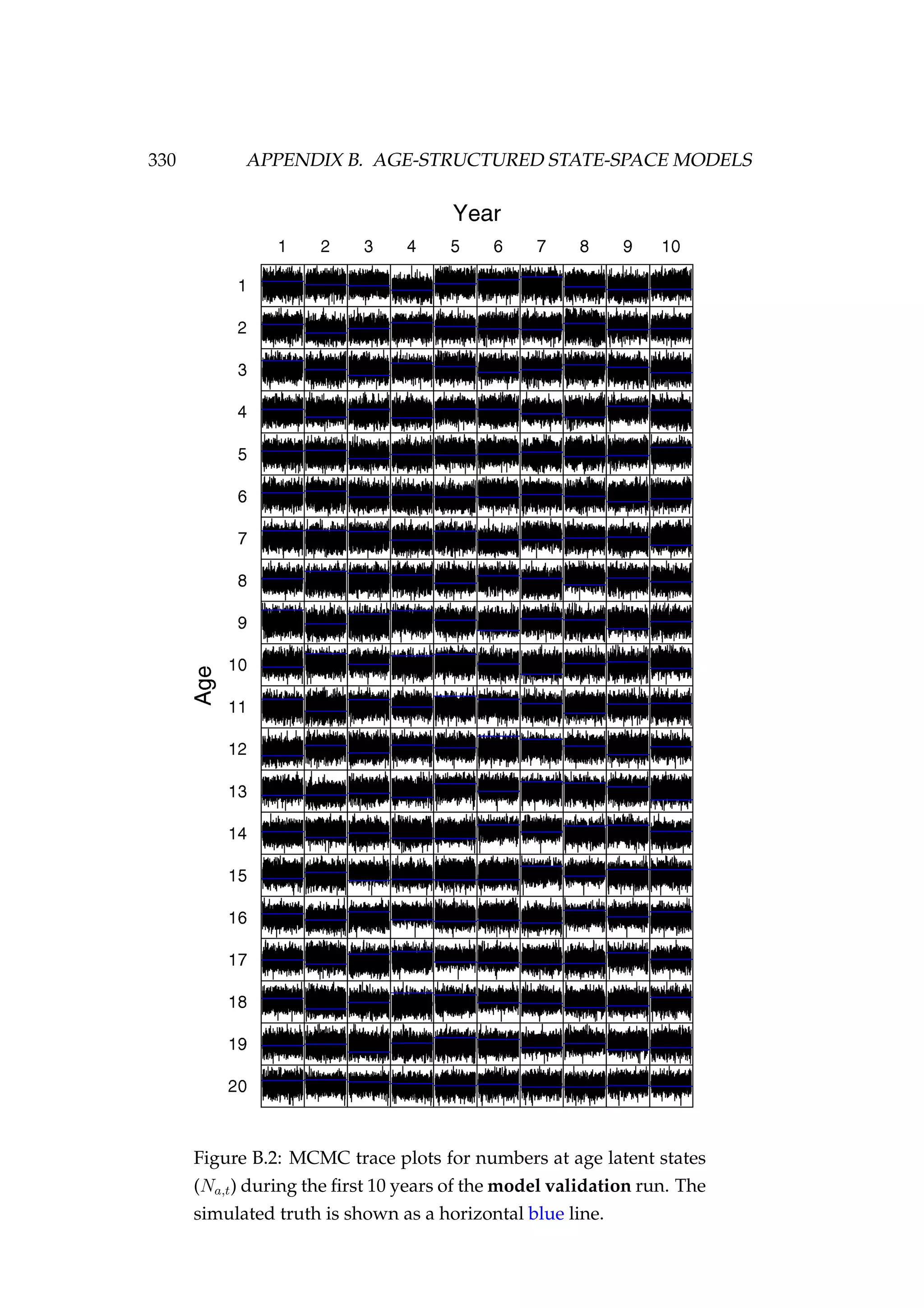
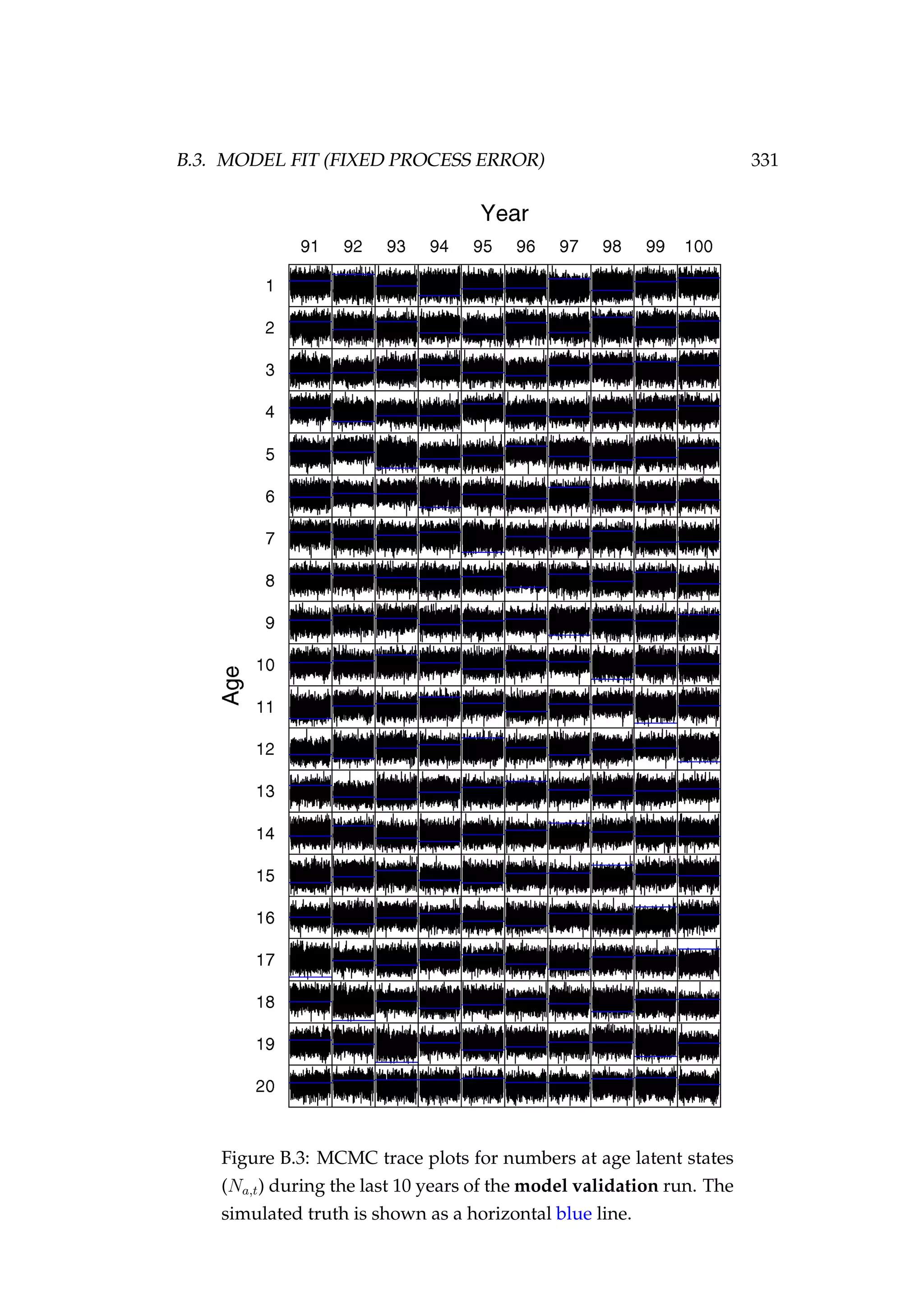
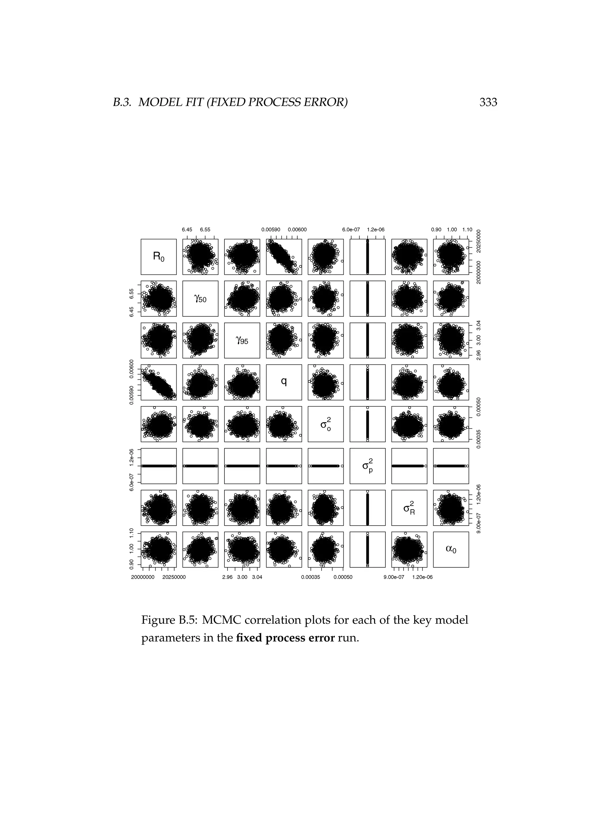
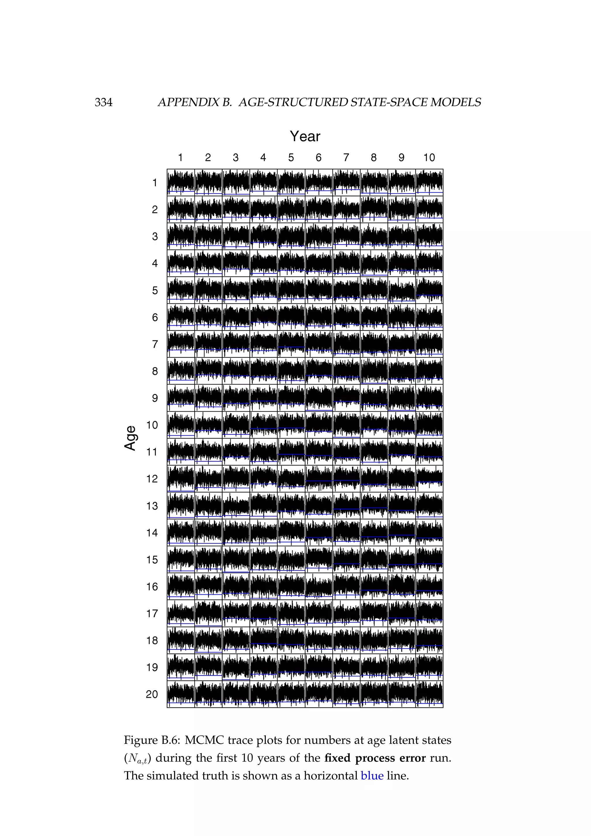
341. B.3. MODEL FIT (FIXED PROCESS ERROR) 329
Figure B.1: MCMC acceptance rates for each of the num-
bers at age and time (Na,t) latent states [bottom] in the model
validation run. It is recommended that the acceptance rate
in Metropolis-Hastings MCMC be between 15 and 50%, this
range is indicated by the dashed lines. The age of the latent
state that each acceptance refers to is indicated numerically (i.e.
the point “1” refers to an age-1 latent state). The colours refer
to each of the two MCMC chains that were run.

342. 330 APPENDIX B. AGE-STRUCTURED STATE-SPACE MODELS
Figure B.2: MCMC trace plots for numbers at age latent states
(Na,t) during the first 10 years of the model validation run. The
simulated truth is shown as a horizontal blue line.

343. B.3. MODEL FIT (FIXED PROCESS ERROR) 331
Figure B.3: MCMC trace plots for numbers at age latent states
(Na,t) during the last 10 years of the model validation run. The
simulated truth is shown as a horizontal blue line.

344. 332 APPENDIX B. AGE-STRUCTURED STATE-SPACE MODELS
Figure B.4: MCMC acceptance rates for each of the model pa-
rameters [top] and each of the numbers at age and time (Na,t)
latent states [bottom] in the fixed process error run. It is rec-
ommended that the acceptance rate in Metropolis-Hastings
MCMC be between 15 and 50%, this range is indicated by the
dashed lines. The age of the latent state that each acceptance
refers to is indicated numerically (i.e. the point “1” refers to an
age-1 latent state). The colours refer to each of the two MCMC
chains that were run.

345. B.3. MODEL FIT (FIXED PROCESS ERROR) 333
Figure B.5: MCMC correlation plots for each of the key model
parameters in the fixed process error run.

346. 334 APPENDIX B. AGE-STRUCTURED STATE-SPACE MODELS
Figure B.6: MCMC trace plots for numbers at age latent states
(Na,t) during the first 10 years of the fixed process error run.
The simulated truth is shown as a horizontal blue line.

347. B.3. MODEL FIT (FIXED PROCESS ERROR) 335
Figure B.7: MCMC trace plots for numbers at age latent states
(Na,t) during the last 10 years of the fixed process error run.
The simulated truth is shown as a horizontal blue line.

348. 336 APPENDIX B. AGE-STRUCTURED STATE-SPACE MODELS
B.4 Model fit (releasing σ2
R)
These plots are relevant to the MCMC that attempted to estimate all but
one of the key parameters (i.e. the process error parameter was fixed at
the value specified in the simulation) and in which a higher recruitment
variance was used. Discussion of this MCMC can be found in Chapter 5
(page 201).

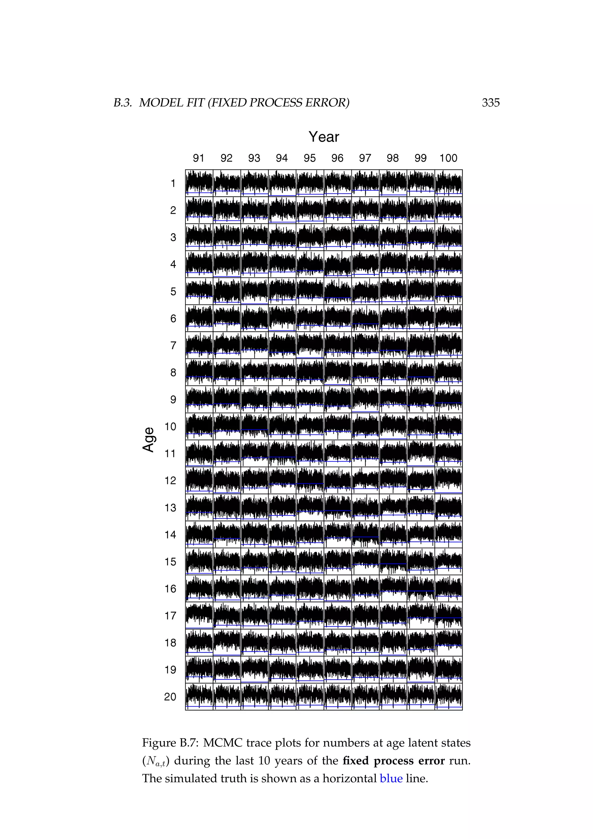
349. B.4. MODEL FIT (RELEASING σ2
R) 337
Figure B.8: MCMC acceptance rates for each of the model pa-
rameters [top] and each of the numbers at age and time (Na,t)
latent states [bottom] in the higher recruitment run. It is rec-
ommended that the acceptance rate in Metropolis-Hastings
MCMC be between 15 and 50%, this range is indicated by the
dashed lines. The age of the latent state that each acceptance
refers to is indicated numerically (i.e. the point “1” refers to an
age-1 latent state). The colours refer to each of the two MCMC
chains that were run.

350. 338 APPENDIX B. AGE-STRUCTURED STATE-SPACE MODELS
Figure B.9: MCMC correlation plots for each of the key model
parameters in the higher recruitment run.

351. B.4. MODEL FIT (RELEASING σ2
R) 339
Figure B.10: MCMC trace plots for numbers at age latent states
(Na,t) during the first 10 years of the higher recruitment run.
The simulated truth is shown as a horizontal blue line.

352. 340 APPENDIX B. AGE-STRUCTURED STATE-SPACE MODELS
Figure B.11: MCMC trace plots for numbers at age latent states
(Na,t) during the last 10 years of the higher recruitment run.
The simulated truth is shown as a horizontal blue line.

353. Appendix C
Pop-up satellite archival tagging
C.1 GPS coordinates for tag 186
Table C.1 gives the GPS coordinates of the towed tag (tag 186).
C.2 MCMC diagnostics
341

354. 342 APPENDIX C. POP-UP SATELLITE ARCHIVAL TAGGING
Table C.1: Date (during February 2012), time, latitude and longitude
recorded along towed tag (tag 186) track.
Date Time Latitude Longitude Date Time Latitude Longitude
22 04:21 -75.750556 168.985556 24 11:00 -68.685000 177.984722
22 05:00 -75.651944 169.168611 24 12:00 -68.500833 178.002222
22 06:00 -75.533611 169.168611 24 13:00 -68.385556 178.018889
22 07:00 -75.419167 169.650278 24 14:00 -68.235000 178.051944
22 09:00 -75.200000 170.118611 24 15:00 -68.085278 178.083611
22 10:00 -75.035833 170.402500 24 16:00 -67.917778 178.118056
22 11:00 -74.935278 170.616944 24 17:00 -67.784167 178.166667
22 12:00 -74.818056 170.850833 24 18:00 -67.635278 178.200556
22 13:00 -74.685833 171.084722 24 19:00 -67.500556 178.219167
22 14:00 -74.567500 171.318333 24 20:00 -67.350000 178.233333
22 15:00 -74.450000 171.550833 24 22:00 -67.035278 178.318889
22 16:00 -74.318333 171.784444 24 23:00 -67.900556 178.366944
22 17:00 -74.184444 172.033333 25 01:00 -66.585556 178.367500
22 18:00 -74.067778 172.268056 25 02:00 -66.451111 178.301667
22 19:00 -73.935833 172.517500 25 03:00 -66.296111 178.235556
22 20:00 -73.752500 172.768611 25 04:00 -66.134722 178.168611
22 22:00 -73.535556 173.235833 25 05:00 -66.000833 178.101389
23 00:10 -73.283333 173.666667 25 06:00 -65.818333 178.016944
23 01:10 -73.135833 173.905000 25 07:00 -65.668333 177.951944
23 02:00 -73.018056 174.100278 25 08:00 -65.551389 177.901944
23 04:00 -72.770833 174.436667 25 09:00 -65.383611 177.834167
23 05:00 -72.651111 174.584444 25 10:00 -65.202222 177.767500
23 06:00 -72.518333 174.750278 25 12:00 -64.951944 177.650556
23 07:20 -72.368333 174.951389 25 13:00 -64.800000 177.569167
23 08:00 -72.285000 175.067778 25 14:00 -64.651667 177.519167
23 10:00 -72.051667 175.384444 25 15:00 -64.518056 177.467222
23 11:00 -71.917500 175.552500 25 16:00 -64.333333 177.385833
23 12:00 -71.769167 175.735556 25 17:00 -64.201389 177.350000
23 13:00 -71.735833 175.851944 25 18:00 -64.066667 177.285833
23 14:00 -71.567778 176.017778 25 22:00 -63.466944 177.035833
23 15:00 -71.434722 176.184444 26 00:00 -63.183889 176.918333
23 16:00 -71.318333 176.334167 26 01:00 -63.034722 176.868611
23 17:00 -71.200000 176.485556 26 02:00 -62.868333 176.816667
23 18:00 -71.068889 176.651111 26 05:00 -62.450278 176.618056
23 19:00 -70.852500 176.816667 26 06:00 -62.284722 176.566944
23 20:00 -70.985000 177.068889 26 07:00 -62.133889 176.502500
24 03:30 -70.800000 177.434722 26 08:00 -61.917500 176.433611
24 05:00 -69.550278 177.500556 26 09:00 -61.816667 176.400000
24 06:00 -69.385000 177.551389 26 10:00 -61.635833 176.335000
24 08:00 -69.101111 177.667222 26 10:30 -61.550000 176.301944
24 09:00 -68.951944 177.716944

355. C.2. MCMC DIAGNOSTICS 343
Table C.2: Model time-step (t), Heidelberger and Welch’s station-
arity test, Geweke Z-score, and the p-value for the Geweke Z-score
for xt and yt of the 2D location (i.e. xt = (xt, yt)) for the model fit
to the towed tag (tag 186). Note that x0 and xT are not included
here as these points are fixed.
Time-step Heidelberger-Welch Geweke Z-score Geweke p-value
x y x y x y
1 passed passed 1.661 0.873 0.097 0.383
2 passed passed 1.696 0.870 0.090 0.384
3 passed passed 1.685 0.862 0.092 0.388
4 passed passed 1.691 0.884 0.091 0.377
5 passed passed 1.665 0.896 0.096 0.370
6 passed passed 1.625 0.856 0.104 0.392
7 passed passed 1.574 0.749 0.116 0.454
8 passed passed 1.506 0.735 0.132 0.462
9 passed passed 1.477 0.702 0.140 0.482
10 passed passed 1.455 0.648 0.146 0.517
11 passed passed 1.426 0.638 0.154 0.524
12 passed passed 1.408 0.599 0.159 0.549
13 passed passed 1.408 0.622 0.159 0.534
14 passed passed 1.461 0.636 0.144 0.525
15 passed passed 1.730 0.823 0.084 0.411
16 passed passed 1.670 1.026 0.095 0.305
17 passed passed 1.589 1.263 0.112 0.206
18 passed passed 1.531 1.531 0.126 0.126
19 passed passed 1.572 1.733 0.116 0.083
20 passed passed 1.051 1.836 0.293 0.066
21 passed passed 0.957 1.886 0.339 0.059
22 passed passed 0.606 1.901 0.545 0.057
23 passed passed 0.133 1.836 0.894 0.066
24 passed passed -0.147 2.042 0.883 0.041
25 passed passed -0.459 1.822 0.646 0.068
26 passed passed -0.156 1.370 0.876 0.171
27 passed passed 0.350 0.691 0.727 0.489
28 passed passed 1.831 -0.172 0.067 0.863
29 passed passed 2.199 -0.894 0.028 0.371
30 passed passed 1.983 -1.333 0.047 0.182
31 passed passed 1.684 -1.606 0.092 0.108
32 passed passed 1.543 -1.881 0.123 0.060
33 passed passed 1.280 -1.891 0.201 0.059

356. 344 APPENDIX C. POP-UP SATELLITE ARCHIVAL TAGGING
Table C.2: Model time-step (t), Heidelberger and Welch’s station-
arity test, Geweke Z-score, and the p-value for the Geweke Z-score
for xt and yt of the 2D location (i.e. xt = (xt, yt)) for the model fit
to the towed tag (tag 186). Note that x0 and xT are not included
here as these points are fixed.
Time-step Heidelberger-Welch Geweke Z-score Geweke p-value
x y x y x y
34 passed passed 1.272 -1.825 0.203 0.068
35 passed passed 1.338 -1.840 0.181 0.066
36 passed passed 1.264 -1.847 0.206 0.065
37 passed passed 1.092 -1.891 0.275 0.059
38 passed passed 1.039 -1.943 0.299 0.052
39 passed passed 0.618 -1.941 0.537 0.052
40 passed passed 0.057 -1.926 0.954 0.054
41 passed passed -0.203 -1.915 0.839 0.056
42 passed passed -0.253 -1.929 0.800 0.054
43 passed passed -0.137 -1.623 0.891 0.104
44 passed passed 0.191 -1.634 0.848 0.102
45 passed passed 0.692 -1.650 0.489 0.099
46 passed passed 1.611 -1.675 0.107 0.094
47 passed passed 1.686 -1.696 0.092 0.090
48 passed passed 0.859 -1.707 0.391 0.088
49 passed passed 0.290 -1.718 0.772 0.086
50 passed passed -0.129 -1.730 0.898 0.084
51 passed passed -0.401 -1.750 0.689 0.080
52 passed passed -0.503 -1.761 0.615 0.078
53 passed passed -0.528 -1.741 0.597 0.082
54 passed passed -0.712 -1.694 0.477 0.090
55 passed passed -0.731 -1.650 0.465 0.099
56 passed passed -0.823 -1.856 0.410 0.063
57 passed passed -0.923 -1.527 0.356 0.127
58 passed passed -1.080 -1.468 0.280 0.142
59 passed passed -1.306 -1.662 0.191 0.096
60 passed passed -1.604 -1.597 0.109 0.110
61 passed passed -1.923 -1.525 0.054 0.127
62 passed passed -2.253 -1.483 0.024 0.138
63 passed passed -2.428 -1.481 0.015 0.139
64 passed passed -2.570 -1.490 0.010 0.136
65 passed passed -2.361 -1.522 0.018 0.128
66 passed passed -2.510 -1.556 0.012 0.120

357. C.2. MCMC DIAGNOSTICS 345
Table C.2: Model time-step (t), Heidelberger and Welch’s station-
arity test, Geweke Z-score, and the p-value for the Geweke Z-score
for xt and yt of the 2D location (i.e. xt = (xt, yt)) for the model fit
to the towed tag (tag 186). Note that x0 and xT are not included
here as these points are fixed.
Time-step Heidelberger-Welch Geweke Z-score Geweke p-value
x y x y x y
67 passed passed -2.722 -1.601 0.006 0.109
68 passed passed -1.966 -1.647 0.049 0.099
69 passed passed -1.440 -1.684 0.150 0.092
70 passed failed -1.271 -1.444 0.204 0.149
71 passed failed -1.404 -1.573 0.160 0.116
72 passed failed -1.275 -1.772 0.202 0.076
73 failed passed -1.650 -1.989 0.099 0.047
74 failed passed -1.788 -2.185 0.074 0.029
75 passed failed -1.649 -2.461 0.099 0.014
76 passed failed -1.877 -2.238 0.061 0.025
77 failed passed -1.952 -2.096 0.051 0.036
Table C.3: Model time-step (t), Heidelberger and Welch’s station-
arity test, Geweke Z-score, and the p-value for the Geweke Z-score
for xt and yt of the 2D location (i.e. xt = (xt, yt)) for the simulated
tag. Note that x0 and xT are not included here as these points are
fixed.
Time-step Heidelberger-Welch Geweke Z-score Geweke p-value
x y x y x y
1 passed passed -0.415 0.048 0.678 0.961
2 passed passed -0.477 0.103 0.634 0.918
3 passed passed -0.529 0.099 0.597 0.921
4 passed passed -0.623 0.104 0.533 0.917
5 passed passed -0.778 0.115 0.437 0.908
6 passed passed -0.815 0.118 0.415 0.906
7 passed passed -0.879 0.117 0.379 0.907
8 passed passed -1.249 0.116 0.212 0.908
9 passed passed -1.371 0.111 0.170 0.912
10 passed passed -1.239 0.119 0.215 0.905
11 passed passed -0.635 0.139 0.526 0.889

358. 346 APPENDIX C. POP-UP SATELLITE ARCHIVAL TAGGING
Table C.3: Model time-step (t), Heidelberger and Welch’s station-
arity test, Geweke Z-score, and the p-value for the Geweke Z-score
for xt and yt of the 2D location (i.e. xt = (xt, yt)) for the simulated
tag. Note that x0 and xT are not included here as these points are
fixed.
Time-step Heidelberger-Welch Geweke Z-score Geweke p-value
x y x y x y
12 passed passed 0.194 0.158 0.846 0.875
13 passed passed 0.649 0.155 0.516 0.877
14 passed passed 0.735 0.143 0.462 0.887
15 passed passed 0.932 0.164 0.351 0.870
16 passed passed 1.058 0.213 0.290 0.832
17 passed passed 0.902 0.291 0.367 0.771
18 passed passed 0.613 0.435 0.540 0.663
19 passed passed 0.372 0.734 0.710 0.463
20 passed passed 0.203 1.236 0.839 0.217
21 passed passed 0.055 1.939 0.956 0.053
22 passed passed -0.049 2.310 0.961 0.021
23 passed passed -0.128 2.190 0.898 0.029
24 passed passed -0.231 2.062 0.817 0.039
25 passed passed -0.316 1.997 0.752 0.046
26 passed passed -0.373 1.774 0.709 0.076
27 passed passed -0.391 1.622 0.696 0.105
28 passed passed -0.413 1.438 0.680 0.150
29 passed passed -0.384 1.240 0.701 0.215
30 passed passed -0.379 1.068 0.705 0.285
31 passed passed -0.370 0.798 0.711 0.425
32 passed passed -0.382 0.666 0.702 0.505
33 passed passed -0.378 0.586 0.706 0.558
34 passed passed -0.366 0.573 0.714 0.567
35 passed passed -0.364 0.473 0.716 0.636
36 passed passed -0.350 0.389 0.726 0.697
37 passed passed -0.330 0.273 0.741 0.785
38 passed passed -0.302 0.165 0.763 0.869
39 passed passed -0.316 0.095 0.752 0.925
40 passed passed -0.401 0.061 0.689 0.951
41 passed passed -0.392 -0.002 0.695 0.999
42 passed passed -0.433 -0.075 0.665 0.940
43 passed passed -0.576 -0.241 0.565 0.810
44 passed passed -0.497 -0.402 0.619 0.688

359. C.2. MCMC DIAGNOSTICS 347
Table C.3: Model time-step (t), Heidelberger and Welch’s station-
arity test, Geweke Z-score, and the p-value for the Geweke Z-score
for xt and yt of the 2D location (i.e. xt = (xt, yt)) for the simulated
tag. Note that x0 and xT are not included here as these points are
fixed.
Time-step Heidelberger-Welch Geweke Z-score Geweke p-value
x y x y x y
45 passed passed -0.276 -0.362 0.783 0.717
46 passed passed 0.210 -0.402 0.834 0.688
47 passed passed 0.367 -0.255 0.713 0.799
48 passed passed 0.257 -0.119 0.797 0.905
49 passed passed 0.293 0.074 0.770 0.941
50 passed passed 0.816 0.185 0.415 0.853
51 passed passed 0.417 0.237 0.677 0.813
52 passed passed 0.291 0.061 0.771 0.951
53 passed passed 0.337 -0.407 0.736 0.684
54 passed passed 0.241 -0.886 0.810 0.376
55 passed passed -0.381 -1.537 0.703 0.124
56 passed passed -0.571 -2.031 0.568 0.042
57 passed passed 0.150 -2.319 0.881 0.020
58 passed passed 1.160 -2.136 0.246 0.033
59 passed passed 0.769 -1.926 0.442 0.054
60 passed passed 0.811 -1.091 0.417 0.275
61 passed passed 1.105 -0.529 0.269 0.597
62 passed passed 0.551 0.005 0.581 0.996
63 passed passed 0.046 0.143 0.963 0.887
64 passed passed -0.022 0.327 0.982 0.743
65 passed passed 0.506 0.115 0.613 0.909
66 passed passed 0.721 -0.137 0.471 0.891
67 passed passed 0.263 -0.283 0.793 0.777
68 passed passed 0.425 -0.436 0.671 0.663
69 passed passed 0.008 -0.501 0.994 0.616
70 passed passed -0.080 -0.612 0.936 0.540
71 passed passed -0.546 -0.769 0.585 0.442
72 passed passed -0.421 -0.962 0.674 0.336
73 passed passed -0.483 -1.180 0.629 0.238
74 passed passed -0.318 -1.293 0.750 0.196
75 passed passed -0.041 -1.372 0.967 0.170
76 passed passed -0.292 -1.545 0.770 0.122
77 passed passed -0.160 -1.289 0.873 0.197

360. 348 APPENDIX C. POP-UP SATELLITE ARCHIVAL TAGGING
Table C.4: Model time-step (t), Heidelberger and Welch’s station-
arity test, Geweke Z-score, and the p-value for the Geweke Z-score
for xt and yt of the 2D location (i.e. xt = (xt, yt)) for the model fit
to the towed tag (tag 121). Note that x0 and xT are not included
here as these points are fixed.
Time-step Heidelberger-Welch Geweke Z-score Geweke p-value
x y x y x y
1 passed passed 0.707 -0.392 0.480 0.695
2 passed passed -1.942 2.452 0.052 0.014
3 passed passed -9.765 7.165 0.000 0.000
4 passed passed -1.016 1.167 0.309 0.243
5 passed passed 2.416 -0.731 0.016 0.464
6 passed passed 1.713 -1.257 0.087 0.209
7 passed passed 1.756 -1.577 0.079 0.115
8 passed passed 1.418 -1.288 0.156 0.198
9 passed passed 0.178 -0.750 0.858 0.453
10 passed passed 0.073 0.598 0.942 0.550
11 passed passed 0.293 -1.300 0.770 0.194
12 passed passed -0.092 1.425 0.927 0.154
13 passed passed -0.360 2.289 0.719 0.022
14 passed passed -1.570 1.301 0.116 0.193
15 passed passed 0.184 -1.334 0.854 0.182
16 passed passed 2.439 -2.276 0.015 0.023
17 passed passed 0.545 -0.753 0.586 0.452
18 passed passed -0.674 0.088 0.500 0.930
19 passed passed -0.733 1.754 0.463 0.079
20 passed passed 0.713 0.121 0.476 0.904
21 passed passed -0.367 -0.580 0.714 0.562
22 passed passed 1.475 -0.855 0.140 0.393
23 passed passed 0.613 -0.451 0.540 0.652
24 passed passed 0.257 0.329 0.797 0.742
25 passed passed -0.397 2.369 0.691 0.018
26 passed passed 0.218 1.325 0.827 0.185
27 passed passed 0.126 0.967 0.900 0.333
28 passed passed -1.787 -1.889 0.074 0.059
29 passed passed 0.208 -0.818 0.835 0.414
30 passed passed 1.121 -1.219 0.262 0.223
31 passed passed 0.047 0.159 0.962 0.874
32 passed passed -0.341 1.092 0.733 0.275

361. C.2. MCMC DIAGNOSTICS 349
Table C.4: Model time-step (t), Heidelberger and Welch’s station-
arity test, Geweke Z-score, and the p-value for the Geweke Z-score
for xt and yt of the 2D location (i.e. xt = (xt, yt)) for the model fit
to the towed tag (tag 121). Note that x0 and xT are not included
here as these points are fixed.
Time-step Heidelberger-Welch Geweke Z-score Geweke p-value
x y x y x y
33 passed passed 1.386 -0.326 0.166 0.744
34 passed passed -0.088 0.663 0.930 0.507
35 passed passed 0.659 -0.071 0.510 0.944
36 passed passed -2.000 3.102 0.045 0.002
37 passed passed 1.565 1.198 0.118 0.231
38 passed passed 0.244 0.766 0.808 0.443
39 passed passed -1.059 1.056 0.290 0.291
40 passed passed 0.748 -0.678 0.454 0.498
41 passed passed -1.624 2.367 0.104 0.018
42 passed passed -0.765 1.468 0.444 0.142
43 passed passed 0.053 -0.185 0.958 0.853
44 passed passed -0.335 0.414 0.737 0.679
45 passed passed -0.366 0.181 0.714 0.856
46 passed passed -0.860 0.453 0.390 0.650
47 passed passed -0.300 -0.685 0.764 0.493

362. 350 APPENDIX C. POP-UP SATELLITE ARCHIVAL TAGGING

363. Appendix D
Agent-based model of snapper
(SNA 1)
This appendix provides input and output from the snapper (SNA 1) agent-
based model (ABM) that was used in the development of Bayesian emula-
tion (described in Chapter 7, page 298). The actual model input file for the
agent-based simulation of snapper (SNA 1) is given, followed by series of
plots of the model output.
D.1 ABM input file
// ==============================================================================
// Species: SNA 1
// ==============================================================================
#ifndef PARAMETERS_H
#define PARAMETERS_H
#define DEBUG_OFF
#define THREADING_ON
#define HOME_ON
// ==============================================================================
// GLOBAL VARIABLES
// ==============================================================================
const int myseed = 7;
const int agent_size = 100;
const int merge_thresh = 10;
351

364. 352 APPENDIX D. AGENT-BASED MODEL OF SNAPPER (SNA 1)
const bool merge_by_age = 1; // If =1 then merge by age, else merge by cell.
const int min_age = 1;
const int max_age = 50;
const int n_stocks = 3;
const int n_areas = 3;
const int n_sex = 2;
const int n_fishery = 1;
const int n_fyears = 114;
const int n_steps = 2;
// ==============================================================================
// INITIALISATION
// ==============================================================================
const int phase1 = 100;
const int phase2 = 100;
// ==============================================================================
// STOCHASTICITY SWITCHES (0 = off, 1 = on)
// ==============================================================================
const bool stochastic_sex = 1;
const bool stochastic_rec = 1;
const bool stochastic_mat = 1;
const bool stochastic_growth = 1;
const bool stochastic_mort = 1;
// ==============================================================================
// RECRUITMENT
//
==============================================================================
// EN, HG, BP
const int R0[n_stocks] = {443493, 950050, 318619};
const double steepness[n_stocks] = {0.85, 0.85, 0.85};
const double p_male[n_stocks] = {0.5, 0.5, 0.5};
const int y_enter[n_stocks] = {1, 1, 1};
const double rec_sigma[n_stocks] = {0.1408, 0.1408, 0.1408};
const double rec_autocorr[n_stocks] = {0.6, 0.6, 0.6};
// ==============================================================================
// MATURITY
// ==============================================================================
// F, M
const double mat_a50[n_sex] = {4, 4};
const double mat_ato95[n_sex] = {4.7, 4.7};
const int mat_L[n_sex] = {3, 3};
const int mat_R[n_sex] = {5, 5};
const double mat_a50_sigma[n_sex] = {0.001, 0.001};
const double mat_ato95_sigma[n_sex] = {0.001, 0.001};
// ==============================================================================
// SIZE
// ==============================================================================
const double size_linf[n_sex]={58.8, 58.8};

365. D.1. ABM INPUT FILE 353
const double size_linf_cv[n_sex]={0.01,0.01};
const double size_k[n_sex]={0.102, 0.102};
const double size_k_sigma[n_sex]={0.001,0.001};
const double size_t0[n_sex]={-1.11, -1.11};
const double size_cv[n_sex]={0.102, 0.102};
const double size_sigma_min[n_sex]={0.001, 0.001};
// ==============================================================================
// LENGTH-WEIGHT
// ==============================================================================
const double size_alpha[n_sex]={4.467e-08, 4.467e-08};
const double size_alpha_sigma[n_sex]={1e-10, 1e-10};
const double size_beta[n_sex]={2.793, 2.793};
const double size_beta_sigma[n_sex]={0.001, 0.001};
// ==============================================================================
// NATURAL MORTALITY
// ==============================================================================
const double mort_M[n_sex]={0.075, 0.075};
const double mort_sigma[n_sex]={0.001, 0.001};
const double mort_dPar = 1; // introduces -ve bias
// ==============================================================================
// FISHERY
// ==============================================================================
const int first_yr[n_fishery]={1900};
const int last_yr[n_fishery]={2013};
const double fish_removals[n_areas][n_fyears]={
{41.6, 53.4, 53.7, 53.9, 54.2, 54.5, 54.8, 55, 55.3, 55.6, 55.9, 56.1, 56.4,
56.7, 57, 57.3, 66.3, 102.4, 93.1, 76.8, 87.4, 94.2, 99.7, 116.9, 132.1,
149.5, 117.9, 142.6, 101.3, 120.2, 127, 92.6, 94.3, 105.8, 115.1, 140,
162.7, 146.8, 158.2, 153.2, 135, 128.2, 112.5, 120.9, 131.6, 129.1, 137.7,
147.4, 168.4, 150, 134.2, 116.8, 105.6, 103.8, 117.8, 121.2, 128.1, 140.2,
137.6, 151.7, 167.9, 177.8, 201.5, 222, 238.6, 265, 292.4, 313.3, 347.7,
361.9, 372.1, 390.5, 360.4, 342.7, 300.6, 246.1, 277, 278.1, 355.9, 380.6,
288.5, 314.1, 300.5, 278, 332, 298.2, 232.1, 129.9, 154.5, 179.9, 225,
149.3, 163.6, 171.8, 183.6, 175.4, 208.8, 203.3, 176.1, 174.3, 169.5, 177.1,
167.3, 162.9, 167.5, 175.6, 212, 200.1, 186, 186.9, 187.2, 177.1, 174.9,
174.9},
{115.8, 150.2, 150.9, 151.7, 152.4, 153.2, 154, 154.7, 155.5, 156.3, 157,
157.8, 158.5, 159.3, 160.1, 160.8, 187.4, 293.5, 266.5, 218.3, 249.2, 270,
285.9, 336.1, 380.8, 432.5, 339.1, 411.5, 289.9, 345.6, 365.8, 264.1, 269,
302.8, 331, 403.8, 470.5, 423.8, 456.9, 442.4, 388.3, 368.2, 322.3, 347,
378.3, 371, 396, 424.7, 486.2, 432.3, 385.2, 334.2, 300.9, 296, 337, 347.4,
367.7, 403.1, 395.8, 436.6, 436.4, 416.9, 438.9, 450.9, 451.7, 480.9,
513.7, 526.6, 580.3, 665.6, 738.9, 789.7, 708, 665.3, 569.1, 455.3, 530.2,
538.7, 688.9, 704.2, 518.7, 540.5, 500, 448.6, 449.9, 459.3, 382.6, 350.8,
454.7, 494.7, 425.4, 445.9, 529.1, 458.1, 433.3, 395.1, 364.1, 359.5,
387.6, 354.3, 344.8, 359.3, 387.5, 407.3, 331.5, 315.9, 343, 352.1, 429.2,
444.3, 416.4, 437.5, 473.4, 473.4},
{52.5, 67.7, 67.9, 68.2, 68.4, 68.6, 68.8, 69, 69.3, 69.5, 69.7, 69.9, 70.1,
70.4, 70.6, 70.8, 82.6, 129.8, 117.7, 95.9, 109.8, 118.8, 125.6, 148.1,
167.9, 190.9, 149, 181.3, 126.8, 151.6, 160.6, 114.9, 117.1, 132.2, 144.5,

366. 354 APPENDIX D. AGENT-BASED MODEL OF SNAPPER (SNA 1)
176.8, 206.5, 185.5, 200.3, 193.6, 169.3, 160.3, 139.7, 150.6, 164.6, 161,
172, 184.4, 212.2, 187.8, 166.9, 143.7, 128.8, 126.6, 144.7, 149.2, 158.4,
173.8, 170.7, 188.7, 200.9, 204.5, 226.7, 244.6, 257.3, 282.6, 309.3,
327.7, 363.9, 390.8, 411.9, 421.6, 372.1, 340.3, 285.4, 223.3, 243.2,
233.7, 284.7, 288.9, 209.4, 216.9, 198.5, 175.6, 156.5, 226.8, 190.2,
122.4, 111.4, 128.8, 159.1, 138.1, 168.6, 153.1, 141.1, 160.2, 195, 205.2,
153.3, 183.8, 223.3, 173.6, 187.8, 234.4, 228.7, 261.1, 245.5, 191.7,
203.5, 185.2, 214.7, 235.5, 229.6, 229.6}
};
const double fish_q=1.08658658658659;
const double fish_q_sigma=0.001;
const double fish_max_exploitation=0.9;
// ==============================================================================
// SELECTIVITY
// ==============================================================================
const int sel_attribute=0; // 0=age, 1=length, 2=weight
const double sel_a1[n_sex] = {6.04604604604605, 6.04604604604605};
const double sel_sL[n_sex] = {2.31481481481481, 2.31481481481481};
const double sel_sR[n_sex] = {100., 100.};
// ==============================================================================
// LAYERS
// ==============================================================================
const char lay_names[n_areas][2] = {
{’E’,’N’},
{’H’,’G’},
{’B’,’P’}
};
const double lay_recruitment[n_stocks][n_areas] = {
{1, 0, 0},
{0, 1, 0},
{0, 0, 1}
};
const int lay_stock[n_areas] = {0, 1, 2};
// ==============================================================================
// MIGRATION
// ==============================================================================
const double mig_matrix[n_areas][n_areas] = {
{0.7696967, 0.0536603, 0.176643},
{0.0870992, 0.5140839, 0.398817},
{0.2408820, 0.2760040, 0.483114}
};
const bool home_rec = 1; // home_rec = 1 if home is the cell that fish recruit to
// ==============================================================================
// TAGGING
// ==============================================================================
const double tag_a1[n_fishery][n_sex] = {
{100., 100.}
};
const double tag_sL[n_fishery][n_sex] = {

367. D.2. PLOTS OF ABM OUTPUT 355
{21., 21.}
};
const double tag_sR[n_fishery][n_sex] = {
{1000., 1000.}
};
const int tag_fish[n_areas][n_fyears] = {
{0, 0, 0, 0, 0, 0, 0, 0, 0, 0, 0, 0, 0, 0, 0, 0, 0, 0, 0, 0, 0, 0, 0, 0, 0,
0, 0, 0, 0, 0, 0, 0, 0, 0, 0, 0, 0, 0, 0, 0, 0, 0, 0, 0, 0, 0, 0, 0, 0, 0,
0, 0, 0, 0, 0, 0, 0, 0, 0, 0, 0, 0, 0, 0, 0, 0, 0, 0, 0, 0, 0, 0, 0, 0, 0,
0, 0, 0, 0, 0, 0, 0, 0, 0, 6782, 0, 0, 0, 0, 0, 0, 0, 0, 8190, 0, 0, 0, 0,
0, 0, 0, 0, 0, 0, 0, 0, 0, 0, 0, 0, 0, 0, 0},
{0, 0, 0, 0, 0, 0, 0, 0, 0, 0, 0, 0, 0, 0, 0, 0, 0, 0, 0, 0, 0, 0, 0, 0, 0,
0, 0, 0, 0, 0, 0, 0, 0, 0, 0, 0, 0, 0, 0, 0, 0, 0, 0, 0, 0, 0, 0, 0, 0, 0,
0, 0, 0, 0, 0, 0, 0, 0, 0, 0, 0, 0, 0, 0, 0, 0, 0, 0, 0, 0, 0, 0, 0, 0, 0,
0, 0, 0, 0, 0, 0, 0, 0, 0, 12046,0, 0, 0, 0, 0, 0, 0, 0, 13466,0, 0, 0, 0,
0, 0, 0, 0, 0, 0, 0, 0, 0, 0, 0, 0, 0, 0, 0},
{0, 0, 0, 0, 0, 0, 0, 0, 0, 0, 0, 0, 0, 0, 0, 0, 0, 0, 0, 0, 0, 0, 0, 0, 0,
0, 0, 0, 0, 0, 0, 0, 0, 0, 0, 0, 0, 0, 0, 0, 0, 0, 0, 0, 0, 0, 0, 0, 0, 0,
0, 0, 0, 0, 0, 0, 0, 0, 0, 0, 0, 0, 0, 0, 0, 0, 0, 0, 0, 0, 0, 0, 0, 0, 0,
0, 0, 0, 0, 0, 0, 0, 0, 0, 0, 0, 0, 0, 0, 0, 0, 0, 0, 3630, 0, 0, 0, 0, 0,
0, 0, 0, 0, 0, 0, 0, 0, 0, 0, 0, 0, 0, 0}
};
#endif /*PARAMETERS_H*/
D.2 Plots of ABM output

368. 356 APPENDIX D. AGENT-BASED MODEL OF SNAPPER (SNA 1)
Figure D.1: Population parameters in the initialised popula-
tion. The dashed red line is the specified median.

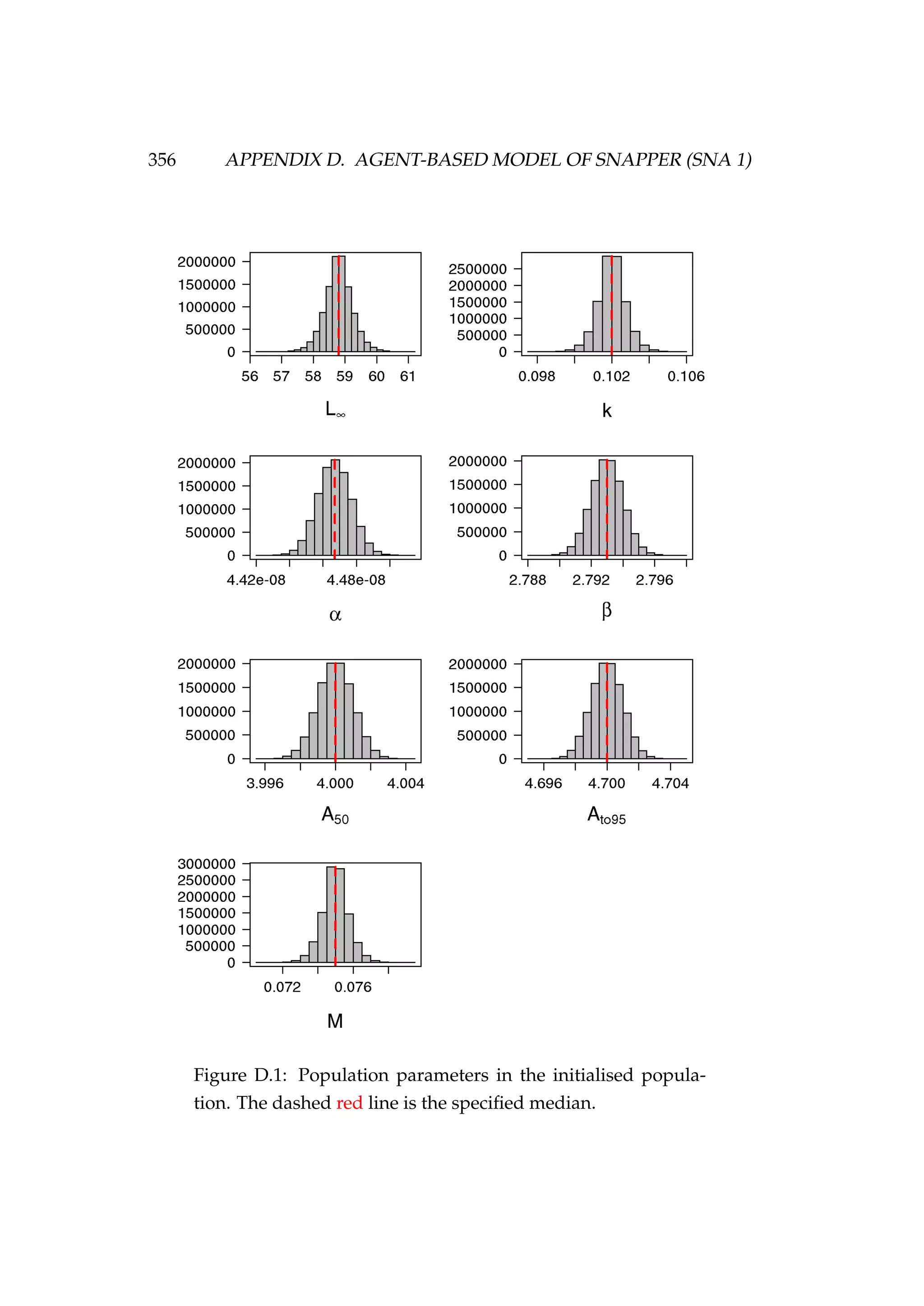
369. D.2. PLOTS OF ABM OUTPUT 357
Figure D.2: Age-length [top left], age-weight [top right] and
length-weight [bottom] of agents in the initialised population.
These plots are split by female and male.

370. 358 APPENDIX D. AGENT-BASED MODEL OF SNAPPER (SNA 1)
Figure D.3: Proportion mature at age for females [top left] and
males [right] and the proportion mature by length [bottom] in
the initialised population.

371. D.2. PLOTS OF ABM OUTPUT 359
Figure D.4: Stock recruitment SR(SSBt) during both phases of
initialisation in East-Northland [top left], the Hauraki Gulf [top
right] and the Bay of Plenty [bottom].

372. 360 APPENDIX D. AGENT-BASED MODEL OF SNAPPER (SNA 1)
Figure D.5: Recruitment Rt during the second phase of initiali-
sation in East-Northland [top left], the Hauraki Gulf [top right]
and the Bay of Plenty [bottom].

373. D.2. PLOTS OF ABM OUTPUT 361
Figure D.6: Spawning stock biomass SSBt during both phases
of initialisation in East-Northland [top left], the Hauraki Gulf
[top right] and the Bay of Plenty [bottom].

374. 362 APPENDIX D. AGENT-BASED MODEL OF SNAPPER (SNA 1)
Figure D.7: Catch (tonnes) that was specified and catch in the
model in East-Northland [top left], the Hauraki Gulf [top right]
and the Bay of Plenty [bottom].

375. D.2. PLOTS OF ABM OUTPUT 363
Figure D.8: The age-frequencies [left column] and the length-
frequencies [right column] in the population during the final
ten years of the fishery.

376. 364 APPENDIX D. AGENT-BASED MODEL OF SNAPPER (SNA 1)
Figure D.9: Biomass (tonnes) in all areas during the fishery
including the total biomass, the vulnerable biomass and the
spawning stock biomass.

377. References
Anderson, L. (1977), The Economics of Fisheries Management, The Blackburn
Press.
Armstrong, J. & Schindler, D. (2011), ‘Excess digestive capacity in preda-
tors reflects a life of feast and famine’, Nature 476, 84–87.
Arreguin-Sanchez, F. (1996), ‘Catchability: a key parameter for fish stock
assessment’, Reviews in Fish Biology and Fisheries 6, 221–242.
Beverton, R. & Holt, S. (1957), On the Dynamics of Exploited Fish Populations,
Vol. 19 of 2, Ministry of Agriculture, Fisheries and Food, London.
Biro, P. & Post, J. (2008), ‘Rapid depletion of genotypes with fast growth
and bold personality traits from harvested fish populations’, PNAS
pp. 2919–2922.
Booth, J. D. (1984), ‘Size at onset of breeding in female Jasus verreauxi (De-
capoda: Palinuridae) in New Zealand’, New Zealand Journal of Marine
and Freshwater Research 18, 159–169.
Booth, J. D. (2011), Spiny Lobsters: Through the Eyes of the Giant Packhorse,
Victoria University Press.
Branch, T. (2009a), ‘Corrigendum: Differences in predicted catch compo-
sition between two widely used catch equation formulations’, Canadian
Journal of Fisheries and Aquatic Science 66, 1631.
Branch, T. (2009b), ‘Differences in predicted catch composition between
two widely used catch equation formulations’, Canadian Journal of Fish-
eries and Aquatic Science 66, 126–132.
Branch, T. (2010), ‘Reply to the comment by Francis on ”Differences in
365

378. 366 REFERENCES
predicted catch composition between two widely used catch equation
formulations”’, Canadian Journal of Fisheries and Aquatic Science 67, 766–
768.
Brasher, D., Ovenden, J., Booth, J. D. & White, R. (1992), ‘Genetic sub-
division of Australian and New Zealand populations of Jasus verreauxi
(Decapoda: Palinuridae) - preliminary evidence from the mitochondrial
genome’, New Zealand Journal of Marine and Freshwater Research 26(1), 53–
58.
Brown, J., Brickle, P. & Scott, B. (2011), ‘Investigating the movements and
behaviour of Patagonian toothfish (Dissostichus eleginoides Smitt, 1898)
around the Falkland Islands using satellite linked archival tags’, Journal
of Experimental Marine Biology and Ecology 443, 65–74.
Bull, B., Francis, R., Dunn, A., McKenzie, A., Gilbert, D., Smith, M., Bian,
R. & Fu, D. (2012), ‘CASAL (C++ algorithmic stock assessment labora-
tory): CASAL User Manual v2.30-2012/03/21’, NIWA Technical Report
135, 280.
Butterworth, D., Ianelli, J. & Hilborn, R. (2003), ‘A statistical model for
stock assessment of southern bluefin tuna with temporal changes in se-
lectivity’, African Journal of Marine Science 25(1), 331–361.
Cadrin, S. X. & Secor, D. (2009), ‘Accounting for spatial population struc-
ture in stock assessment: past, present, and future’, Fish and Fisheries
31, 405–426.
Davey, F. (2004), Ross Sea Bathymetry, 1:2 000 000, version 1.0, Institute of
Geological and Nuclear Sciences geophysical map 16, Technical report,
Institute of Geological and Nuclear Sciences Limited.
Diggle, P., Heagerty, P., Liang, K. & Zeger, S. (2002), Analysis of Longitudinal
Data, 2nd edn, Oxford University Press.
Dunn, A. & Hanchet, S. (2011), ‘Southern blue whiting (Micromesistius aus-
tralis) stock assessment for the Campbell Island Rise for 2009-10’, New
Zealand Fisheries Assessment Report 2011/40, 37.
Dunn, A. & Rasmussen, S. (2009), Spatial Population Model User Manual

379. 367
(SPM v0.1-2009-02-04-23:08:28 UTC (rev. 2987)), National Institute of Wa-
ter & Atmospheric Research Ltd.
Dunn, A., Rasmussen, S. & Hanchet, S. (2009), ‘Development of spa-
tially explicit age-structured population dynamics operating models for
Antarctic toothfish in the Ross Sea’, WG-SAM 09/18, 38.
Fox, W. (1970), ‘An exponential surplus-yield model for optimizing ex-
ploited fish populations’, Transactions of the American Fisheries Society
99, 80–88.
Francis, R. (1999), ‘The impacts of correlations in standardised CPUE in-
dices’, New Zealand Fisheries Assessment Research Document 1999/42, 30.
Francis, R. (2006), ‘Assessment of hoki (Macruronus novaezelandiae) in
2005’, New Zealand Fisheries Assessment Report 2006/3, 96.
Francis, R. (2010), ‘Comment on ”Differences in predicted catch composi-
tion between two widely used catch equation formulations”’, Canadian
Journal of Fisheries and Aquatic Science 67, 763–765.
Francis, R. (2011), ‘Data weighting in statistical fisheries stock assessment
models’, Canadian Journal of Fisheries and Aquatic Science 68, 1124–1138.
Francis, R. (2014), ‘Replacing the multinomial in stock assessment models:
a first step’, Fisheries Research 151, 70–84.
Francis, R. & McKenzie, A. (2013), ‘Assessment of the SNA 1 stocks in
2013’, New Zealand Fisheries Assessment Report .
Gelman, A. (2006), ‘Prior distributions for variance parameters in hierar-
chical models’, Bayesian Analysis 1(3), 515–533.
Geman, S. & Geman, D. (1984), ‘Stochastic relaxation, Gibbs distributions
and the Bayesian restoration of images’, IEEE Transactions on Pattern
Analysis and Machine Intelligence 6, 721–741.
Gilks, W. & Roberts, C. (1996), Strategies for improving MCMC, Chapman &
Hall, pp. 89–114.
Godo, O. & Michalsen, K. (2000), ‘Migratory behaviour of north-east Arctic
cod, studied by use of data storage tags’, Fisheries Research 48, 127–140.

380. 368 REFERENCES
Goldstein, M. & Rougier, J. (2006), ‘Bayes linear calibrated prediction
for complex systems’, Journal of the American Statistical Association
101(475), 1132–1143.
Gray, R., Fulton, B., Little, R. & Scott, R. (2006), Ecosystem model specifi-
cation with an agent based framework, Technical report, CSIRO.
Green, P. (1995), ‘Reversible jump Markov chain Monte Carlo computation
and Bayesian model determination’, Biometrika 82(4), 711–732.
Grimm, V. & Railsback, S. (2005), Individual-Based Modeling and Ecology,
Princeton University Press.
Haist, V., Breen, P. A., Starr, P. J. & Kendrick, T. H. (2011), ‘The 2010 stock
assessment of red rock lobsters (Jasus edwardsii) in CRA 5, and develop-
ment of an operational management procedure’, New Zealand Fisheries
Assessment Report 2011/12, 68.
Hanchet, S., Rickard, G., Fenaughty, J., Dunn, A. & Williams, M. (2008), ‘A
hypothetical life cycle for Antarctic toothfish Dissostichus mawsoni in the
Ross Sea region’, CCAMLR Science 15, 35–53.
Hankin, R. (2005), ‘Introducing BACCO, an R package for Bayesian anal-
ysis of computer code output’, Journal of Statistical Software 14(16), 1–21.
Hankin, R. (2012), ‘Introducing multivator: a multivariate emulator’, Jour-
nal of Statistical Software 46(8), 1–20.
Harley, S., Myers, R. & Dunn, A. (2001), ‘Is catch-per-unit-effort propor-
tional to abundance?’, Canadian Journal of Fisheries and Aquatic Science
58, 1760–1772.
Harwood, J. & Stokes, K. (2003), ‘Coping with uncertainty in ecological ad-
vice: lessons from fisheries’, Trends in Ecology and Evolution 18(12), 617–
622.
Hastings, W. (1970), ‘Monte Carlo Sampling methods using Markov chains
and their applications’, Biometrika 57(1), 97–109.
Haylock, R. & O’Hagan, A. (1996), On inference for outputs of computaion-

381. 369
ally expensive algorithms with uncertainty on the inputs, Oxford University
Press, pp. 629–637.
Henderson, D., Boys, R., Krishnan, K., Lawless, C. & Wilkinson, D. (2009),
‘Bayesian emulation and calibration of a stochastic computer model of
mitochondrial DNA deletions in substantia nigra neurons’, Journal of the
American Statistical Association 104(485), 76–87.
Hewitt, D., Lambert, D., Hoenig, J. & Lipcius, R. (2007), ‘Direct and indi-
rect estimates of natural mortality for Chesapeake Bay blue crab’, Trans-
actions of the American Fisheries Society 136, 1030–1040.
Hilborn, R. (2003), ‘The state of the art in stock assessment: where we are
and where we are going’, Scientia Marina 67(1), 15–20.
Hilborn, R. & Kennedy, R. B. (1992), ‘Spatial pattern in catch rates: A test
of economic theory’, Bulletin of Mathematical Biology 54(23), 263–273.
Hilborn, R. & Mangel, M. (1997), The Ecological Detective: Confronting Mod-
els with Data, Princeton Universtiy Press.
Hilborn, R. & Walters, C. J. (1992), Quantitative Fisheries Stock Assessment:
Choice, Dynamics and Uncertainty, Chapman and Hall.
Horodysky, A., Kerstetter, D., Latour, R. & Graves, J. (2007), ‘Habitat uti-
lization and vertical movements of white marlin (Tetrapturus albidus) re-
leased from commercial and recreational fishing gears in the western
North Atlantic Ocean: inferences from short duration pop-up archival
satellite tags’, Fisheries Oceanography 16(3), 240–256.
Hoshino, E., Milner-Gulland, E. & Hillary, R. (2014), ‘Why model assump-
tions matter for natural resource management: interactions between
model structure and life history in fisheries models’, Journal of Applied
Ecology 51(3), 632–641.
Ianelli, J., Honkalehto, T., Barbeaux, S., Kotwicki, S., Aydin, K. &
Williamson, N. (2013), ‘Assessment of the walleye pollock stock in the
Eastern Bering Sea’, NPFMC Bering Sea and Aleutian Islands SAFE pp. 53–
152.
Ianelli, J. & McAllister, M. (1997), ‘Bayesian stock assessment using catch-

382. 370 REFERENCES
age data and the sampling-importance resampling algorithm’, Canadian
Journal of Fisheries Aquatic Science 54(2), 284–300.
Jonsen, I., Basson, M., Bestley, S., Bravington, M., Patterson, T., Pedersen,
M., Thomson, R., Thygesen, U. & Wotherspoon, S. (2013), ‘State-space
models for bio-loggers: a methodological roadmap’, Deep-sea Research II
88, 34–46.
Jorgensen, C. & Fiksen, O. (2006), ‘State-dependent energy allocation in
cod (Gadus morhua)’, Canadian Journal of Fisheries Aquatic Science 63, 186–
199.
Kennedy, M. & O’Hagan, A. (2000), ‘Predicting the output from a com-
plex computer code when fast approximations are available’, Biometrika
87(1), 1–13.
Kensler, C. B. & Skrzynski, W. (1970), ‘Commercial landings of the spiny
lobster Jasus verreauxi in New Zealand (Crustacea: Decapoda: Palinuri-
dae)’, New Zealand Journal of Marine and Freshwater Research 4, 46–54.
Kim, S., Breen, P. A. & Andrew, N. L. (2002), Evaluation of the paua stock
assessment model with an individual-based operating model, Technical
report, National Institute of Water and Atmospheric Research Ltd.
Lambert, P. C., Sutton, A. J., Burton, P. R., Abrams, K. R. & Jones, D. R.
(2005), ‘How vague is vague? A simulation study of the impact of the
use of vague prior distributions in MCMC using WinBUGS’, Statistics in
Medicine 24(15), 2401–2428.
Little, R., Fulton, E., Gray, R., Hayes, D., Lyne, V., Scott, R., Sainsbury,
K. & McDonald, D. (2006), Management strategy evaluation results and
discussion for Australia’s North West Shelf, Technical report, CSIRO.
Magnusson, A. & Hilborn, R. (2007), ‘What makes fisheries data informa-
tive?’, Fish and Fisheries 8, 337–358.
Magnusson, A., Punt, A. & Hilborn, R. (2013), ‘Measuring uncertainty in
fisheries stock assessment: the delta method, bootstrap, and MCMC’,
Fish and Fisheries 14(3), 325–342.
Mangel, M., Brodziak, J. & DiNardo, G. (2010), ‘Reproductive ecology and

383. 371
scientific inference of steepness: a fundamental metric of population dy-
namics and strategic fisheries management’, Fish and Fisheries 11(1), 89–
104.
Marin, J.-M. & Robert, C. P. (2010), Bayesian Core: A Practical Approach to
Computational Bayesian Statistics, Springer.
Maunder, M. & Harley, S. (2011), ‘Using cross validation model selection
to determine the shape of nonparametric selectivity curves in fisheries
stock assessment models’, Fisheries Research 110(2), 283–288.
McAllister, M. K., Pikitch, E. & Babcock, E. (2001), ‘Using demographic
methods to construct Bayesian priors for the intrinsic rate of increase
in the Schaefer model and implications for stock rebuilding’, Canadian
Journal of Fisheries and Aquatic Science 58(9), 1871–1890.
McKay, M., Conover, W. & Beckman, R. (1979), ‘Comparison of three meth-
ods for selecting values of input variables in the analysis of output from
a computer code’, Techonometrics 21, 239–245.
Mertz, G. & Myers, R. (1996), ‘An extended cohort analysis: incorporating
the effect of seasonal catches’, Canadian Journal of Fisheries Aquatic Science
53, 159–163.
Metropolis, N., Rosenbluth, A., Rosenbluth, M., Teller, A. & Teller, E.
(1953), ‘Equation of state calculations by fast computing machines’, Jour-
nal of Chemical Physics 21, 1087–1091.
Meyer, R. & Millar, R. (1999), ‘Bugs in Bayesian stock assessments’, Cana-
dian Journal of Fisheries and Aquatic Science 56, 1078–1087.
Millar, R. & Meyer, R. (2000), ‘Bayesian state-space modeling of age-
structured data: fitting a model is just the beginning’, Canadian Journal
of Fisheries Aquatic Science 57, 43–50.
Ministry for Primary Industries (2014a), Fisheries Assessment Plenary,
May 2014: stock assessments and stock status, Technical report, MPI.
Ministry for Primary Industries (2014b), Fisheries Assessment Plenary,
November 2014: stock assessments and stock status, Technical report,
MPI.

384. 372 REFERENCES
Montgomery, S., Liggins, G., Craig, J. & McLeod, J. (2009), ‘Growth of
the spiny lobster Jasus verreauxi (Decapoda: Palinuridae) off the east
coast of Australia’, New Zealand Journal of Marine and Freshwater Research
43(1), 113–123.
Moore, E. (1920), ‘On the reciprocal of the general algebraic matrix’, Bul-
letin of the American Mathematical Society 26(9), 394–395.
Mormede, S. & Dunn, A. (2013), ‘Investigation of potential biases in the
assessment of Antarctic toothfish in the Ross Sea fishery using outputs
from a spatially explicit operating model’, WG-SAM 13/36, 9.
Mormede, S. & Dunn, A. (2014), ‘A stock assessment model of Antarc-
tic toothfish (Dissostichus mawsoni) in the Ross Sea region incorporating
multi-year mark-recapture data’, CCAMLR Science 21, 39–62.
Mormede, S., Dunn, A. & Hanchet, S. (2011), ‘Assessment models for
Antarctic toothfish (Dissostichus mawsoni) in the Ross Sea for the years
1997-98 to 2010-11’, WG-FSA 11/42, 40.
Mormede, S., Dunn, A. & Hanchet, S. (2013), ‘Assessment models for
Antarctic toothfish (Dissostichus mawsoni) in the Ross Sea for the years
1997-98 to 2010-13’, WG-FSA 13/51, 36.
Mormede, S., Dunn, A., Parker, S. & Hanchet, S. (2013), ‘Further devel-
opment of a spatially explicit population dynamics operating model for
Antarctic toothfish in the Ross Sea region’, WG-SAM 13/35, 21.
Neilsen, A., Bigelow, K., Musyl, M. & Sibert, J. (2006), ‘Improving
light-based geolocation by including sea surface temperature’, Fisheries
Oceanography 15, 314–325.
Nelder, J. & Wedderburn, R. (1972), ‘Generalised linear models’, Journal of
the Royal Statistical Society: Series A 137, 370–384.
Nielsen, A. & Berg, C. W. (2014), ‘Estimation of time-varying selectivity in
stock assessments using state-space models’, Fisheries Research 158, 96–
101.
Oakley, J. (1999), Bayesian Uncertainty Analysis for Complex Computer
Codes, PhD thesis, School of Mathematics and Statistics.

385. 373
Oakley, J. (2004), ‘Estimating percentiles of uncertain computer code out-
puts’, Applied Statistics 53, 83–93.
Oakley, J. & O’Hagan, A. (2002), ‘Bayesian inference for the uncertainty
distribution of computer model outputs’, Biometrika 89, 769–784.
Oakley, J. & O’Hagan, A. (2004), ‘Probabilistic sensitivity analysis of com-
plex models: a Bayesian approach’, Journal of the Royal Statistical Society:
Series B 66, 751–769.
Parker, S., Dunn, A., Mormede, S. & Hanchet, S. (2013), ‘Descriptive anal-
ysis of the toothfish (Dissostichus spp.) tagging programme in Subareas
88.1 & 88.2 for the years 2000-01 to 2012-13’, WG-FSA 13/49, 35.
Parker, S., Hanchet, S. & Horn, P. (2014), ‘Stock structure of Antarctic
toothfish in Statistical Area 88 and implications for assessment and man-
agement’, WG-SAM 14/26.
Parker, S., Webber, D. & Arnold, R. (2014), ‘Deployment and recovery of an
archival tag on an Antarctic toothfish in the Ross Sea’, WG-FSA 14/64, 16.
Patterson, H. & Thompson, R. (1971), ‘Recovery of inter-block information
when block sizes are unequal’, Biometrika 58, 545–554.
Pella, J. & Tomlinson, P. (1969), ‘A generalised stock-production model’,
Bulletin of the Inter-America Tropical Tuna Commision 13, 421–458.
Penrose, R. (1955), ‘A generalized inverse for matrices’, Proceedings of the
Cambridge Philosophical Society 51, 406–413.
Pope, J. (1972), ‘An investigation of the accuracy of Virtual Population
Analysis using cohort analysis’, International Commission for the North-
west Atlantic Fisheries Research Bulletin 9, 65–74.
Press, W., Flannery, B., Teukolsky, S. & Vetterling, W. (1986), Numerical
Recipes: the Art of Scientific Computing, Cambridge University Press.
Prince, J. (2003), ‘The barefoot ecologist goes fishing’, Fish and Fisheries
4, 359–371.
Punt, A. (2003a), ‘Extending production models to include process error

386. 374 REFERENCES
in the population dynamics’, Canadian Journal of Fisheries Aquatic Science
60, 1217–1228.
Punt, A. (2003b), ‘The performance of a size-structured stock assessment
method in the face of spatial heterogeneity in growth’, Fisheries Research
65, 391–409.
Punt, A., Hurtado-Ferro, F. & Whitten, A. (2014), ‘Model selection for se-
lectivity in fisheries stock assessments’, Fisheries Research 158, 124–134.
Quinn, T. (1992), ‘Ruminations on the development and future of popula-
tion dynamics models in fisheries’, Natural Resource Modeling 16(4), 341–
392.
Ralston, S. & O’Farrell, M. (2008), ‘Spatial variation in fishing intensity
and its effect on yield’, Canadian Journal of Fisheries and Aquatic Science
65, 588–599.
Rencher, A. (2000), Linear Models in Statistics, Wiley.
Richards, F. (1959), ‘A flexible growth function for empirical use’, Journal
of Experimental Botany 10(2), 290–301.
Ricker, W. (1954), ‘Stock and recruitment’, Journal of the Fisheries Research
Board of Canada 11, 559–623.
Ridgeway, K., Dunn, J. & Wilkin, J. (2002), ‘Ocean interpolation by four-
dimensional least squares - application to the waters around Australia’,
Journal of Atmospheric and Oceanic Technology 19(9), 1357–1375.
Schaefer, M. B. (1954), ‘Some aspects of the dynamics of populations im-
portant to the management of the commercial marine fisheries’, Bulletin
of Mathematical Biology 1(2), 25–56.
Scheffer, M., Baveco, J., DeAngelis, D., Rose, K. A. & van Nes, E. (1995),
‘Super-individuals a simple solution for modelling large populations on
an individual basis’, Ecological Modelling 80, 161–170.
Schnute, J. (1987), ‘Data, uncertainty, model ambiguity, and model identi-
fication’, Natural Resource Modeling 2, 159–212.

387. 375
Seber, G. (1982), The Estimation of Animal Abundance and Related Parameters,
Blackburn Press.
Seitz, A., Wilson, D., Norcross, B. & Neilsen, J. (2005), ‘Pop-up Archival
Transmitting (PAT) tags: a method to investigate the migration and be-
haviour of Pacific halibut Hippoglossus stenolepis in the Gulf of Alaska’,
Alaska Fisheries Research Bulletin 10, 124–136.
Shelton, A., Satterthwaite, W., Beakes, M., Munch, S., Sogard, S. &
Mangel, M. (2013), ‘Separating intrinsic and environmental contribu-
tions to growth and their population consequences’, American Naturalist
181(6), 799–814.
Siler, J., Foris, W. & McInerny, M. (1986), Spatial heterogeneity in fish pa-
rameters within a reservoir, in G. Hall & M. Van Den Avyle, eds, ‘Reser-
voir Fisheries Management: Strategies for the 80’s’, pp. 122–136.
Smallegange, I. & Coulson, T. (2012), ‘Towards a general, population-level
understanding of eco-evolutionary change’, Trends in Ecology and Evolu-
tion 28, 143–148.
Snyder, J. (1926), Map projections - a working manual.
Stephenson, R. (1999), ‘Stock complexity in fisheries management: a per-
spective of emerging issues related to population sub-units’, Fisheries
Research 43, 247–249.
Stevenson, M., Hanchet, S., Mormede, S. & Dunn, A. (2011), ‘A characteri-
sation of the toothfish fishery in Subareas 88.1 and 88.2 from 1997-98 to
2010-11’, WG-FSA 11/45, 31.
Taylor, I. & Methot, R. (2013), ‘Hiding or dead? A computationally efficient
model of selective fisheries mortality’, Fisheries Research 142, 75–85.
Teo, S., Boustany, A., Blackwell, S., Walli, A., Weng, K. & Block, B. (2004),
‘Validation of geolocation estimates based on light level and sea surface
temperature from electronic tags’, Marine Ecology Progress Series 283, 81–
98.
Thorson, J., Stewart, I. & Punt, A. (2012), ‘Development and application of
an agent-based model to evaluate methods for estimating relative abun-

388. 376 REFERENCES
dance indices for shoaling fish such as Pacific rockfish (Sebastes spp.)’,
ICES Journal of Marine Science .
Vernon, I., Goldstein, M. & R., B. (2010), ‘Galaxy formation: a Bayesian
uncertainty analysis’, Bayesian Analysis 5(4), 619–670.
von Bertalanffy, L. (1934), ‘Untersuchungen uber die Gesetzlichkeiten des
Wachstums I. Allgemeine Grundlagen der Theorie, mathematische und
physiologische Gesetzlichkeiten des Wachstum bei Wassertieren’, Wil-
helm Roux’ Arch. Entwicklungsmech. Org. 131, 613–652.
Walters, C. J. & Hilborn, R. (1976), ‘Adaptive control of fishing systems’,
Journal of the Fisheries Research Board of Canada 33, 145–159.
Webber, D. (2013), ‘Characterisation, catch per unit effort standardisation,
and exploring alternative minimum legal sizes of packhorse rock lob-
sters in New Zealand’, Unpublished p. 51.
Webber, D. & Thorson, J. (2015), ‘Variation in growth among individu-
als and over time: a case study and simulation experiment involving
tagged Antarctic toothfish’, Fisheries Research XX(X).
Welch, D. & Eveson, J. (1999), ‘An assessment of light-based geoposition
estimates form archival tags’, Canadian Journal of Fisheries Aquatic Science
56, 1317–1327.
Williams, R. & Lamb, T. (2002), ‘Behaviour of Dissostichus eleginoides fit-
ted with archival tags at Heard Island: preliminary results’, WG-FSA
02/60, 16.
Wolf, M. & Weissing, F. (2012), ‘Animal personalities: consequences for
ecology and evolution’, Trends in Ecology and Evolution 27, 452–461.