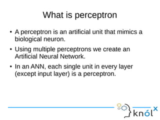
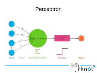
The document provides an overview of machine learning and artificial neural networks, detailing concepts such as perceptrons, activation functions, training and error, and backpropagation. It highlights the importance of these components in creating effective neural networks and discusses various machine learning techniques. Additionally, it addresses the limitations and potential biases present in machine learning applications.

1. Machine Learning
With
Neural Networks
Anuj Saxena
Software Consultant
Knoldus Software LLP

2. Artificial Intelligence: Brief History

3. Agenda
• Machine Learning – what and why?
• ANN - Introduction
• Activation Function
• Train & Error
• Gradient Descent
• Importance of layers
• Back propogation
• Cons
• Demo

4. SKYNET

5. Machine learning
● Machine learning is the subfield of computer
science that gives computers the ability to
learn without being programmed.

7. Machine Learning techniques
● Decision tree
● Random Forests
● K means Clustering
● Naive Bayes Classifier
● Artificial Neural Networks

8. Artificial Neural
Network

9. How the brain works

10. At granular level
perceptron

11. What is perceptron
● A perceptron is an artificial unit that mimics a
biological neuron.
● Using multiple perceptrons we create an
Artificial Neural Network.
● In an ANN, each single unit in every layer
(except input layer) is a perceptron.

12. Perceptron

13. A simple neural network

14. A bit simpler

15. Self Drive Car: ALVINN
● Stands for Autonomous Land Vehicle
In a Neural Network
● Steering a vehicle
● Taking input from
a 30X32 sensor
● Hence, 30X32 units
in input layer
● These inputs are provided
to our neural net and the
output tells us which neuron
to fire from all output neurons
(where each neuron defines
a direction)

16. Activation Function
● The activation function is the last step of
processing in a perceptron.
● It takes the summation of multiplication of the
inputs and their corrosponding weights

17. Need for activation
• Consider the following
• Here value of Y ranges from -inf to +inf
• Hence how to decide whether the neuron should be
fired(activated) or not??
• So we got some activation functions with us
• Step Function
• Linear Function
• Sigmoid Function

18. Step function
• A threshold based activation function
• “activated” if Y > threshold else not
• In this picture
output is 1 ( activated) when
value > 0 (threshold)
and outputs a 0 ( not activated) otherwise
• Drawbacks:
• Can work wrong if using more that two classes (if more than one neuron outputs
activated)
• Multiple layer not supported

19. Linear Function
● Y = c * (summation + bias)
where summation = sum(input*weight)
● A linear function in form of
y = mx
● Not binary in nature
● Drawbacks
– Unbounded
– Can not use multiple layers with this too

20. Sigmoid
● Looks smooth
● Like step function
● Most widely used
● Benefits
– Nonlinear
– Bounded values

21. Sigmoid contd.
● As we are working in bounded outputs, our activation
functions have a range(0, 1)
i.e. our activations are bounded
● Although bounded but not binary in nature
● i.e. we can take the max ( or softmax) in case of more than
one neurons activated.
● As it is non linear in nature hence we can use mutiple layers
to effectively.

22. What is bias?
● The main function of a bias is to provide every node with a
trainable constant value (in addition to the normal inputs
that the node receives)
● Lets consider a simple network with 1 input and 1 output
● The output of the network is computed by multiplying the
input (x) by the weight (w0) and passing the result through
some kind of activation function (e.g. a sigmoid function.)

23. Bias(contd.)
● If we change the values
of w0 the graph
fluctuates like this
●
Changing the weight
w0 essentially changes
the "steepness" of
the sigmoid
● But what if you wanted
the network to output 0
when input (x) is 2?
● changing the steepness
of the sigmoid won't
really work we need to
shift the entire curve
to the right.

24. Bias(contd.)
● Now consider this network with added bias
● The output of the network becomes sig(w0*x +
w1*1.0)
● Here the value of the bias is taken as 1.0

25. Bias(contd.)
● Now the graph moves
something like this with
the change in bias
● Having a weight of -5
for w1 shifts the curve
to the right,
which allows us to
have a network that
outputs 0 when x is 2.

26. Train & Error
● We now know that our perceptrons depend on its
weight vector to provide an output.
● In the training phase we shift the weights for each
input until we get our desired output
● In simple cases and less number of inputs we
can manually change our weights till the limit our
training data satisfies the outputs
● But what if the inputs are very large and training
data is really big too (a real time scenario)

27. Error
● Finding error implies that if we have set our weights in
our ANN model and now we want to check if they are
correct or not?
● An ideal case can not be found when there is no error in
the weight vector. So there will always be some error in
our model.
● i.e. Error = (expected output – gained output)
● Here comes the tolerance(how much error is acceptable)
● i.e. till when we need to update the weights

28. Minimizing Error through Gradient
Descent
● What is gradient??
Ans: An increase or decrease in the magnitude of a property observed in
passing from one point or moment to another
Or
In mathematics, the gradient is a multi-variable generalization of the
derivative.
● Error = - Y
● Squared error function E(w) = 1/2
● Gradient
● Weight update: where

29. Issue with gradient descent
● Gradient descent works fine only with single
layer models (why???)
● But for multilayer???
● Here comes the back propogation

30. Leftovers

31. Layers
● Problems that require two hidden layers are
rarely encountered as neural networks with two
hidden layers can represent functions with any
kind of shape.
● Currently no theoretical reason to use neural
networks with any more than two hidden layers.
● Most problem can be solved using only one
hidden layer.

32. Standards
● The number of neurons in a hidden layer:

33. Back Propogation
● We can find error in weights between hidden layer and the
output layer
● Problem is finding the error in weights between input layer and
hidden layer (and between one hidden layer to another hidden
layer in case of multiple hidden layers)
● For that we have back propogation
● In back propogation we find the error at the output layer and
then use that error to calculate error at the hidden layer.

35. Algorithm

36. Algorithm contd.

37. Output layer

38. Hidden Layer

39. Weight Change

40. Cons
● Google’s Photos app mistakenly tagged two
black people in a photograph as “gorillas.”
● Flickr’s smart new image recognition tool,
powered by Yahoo’s neural network, also
tagged a black man as an “ape.”

41. Demo

42. References
● Machine Learning – Tom Mitchell
● http://www.theprojectspot.com/tutorial-post