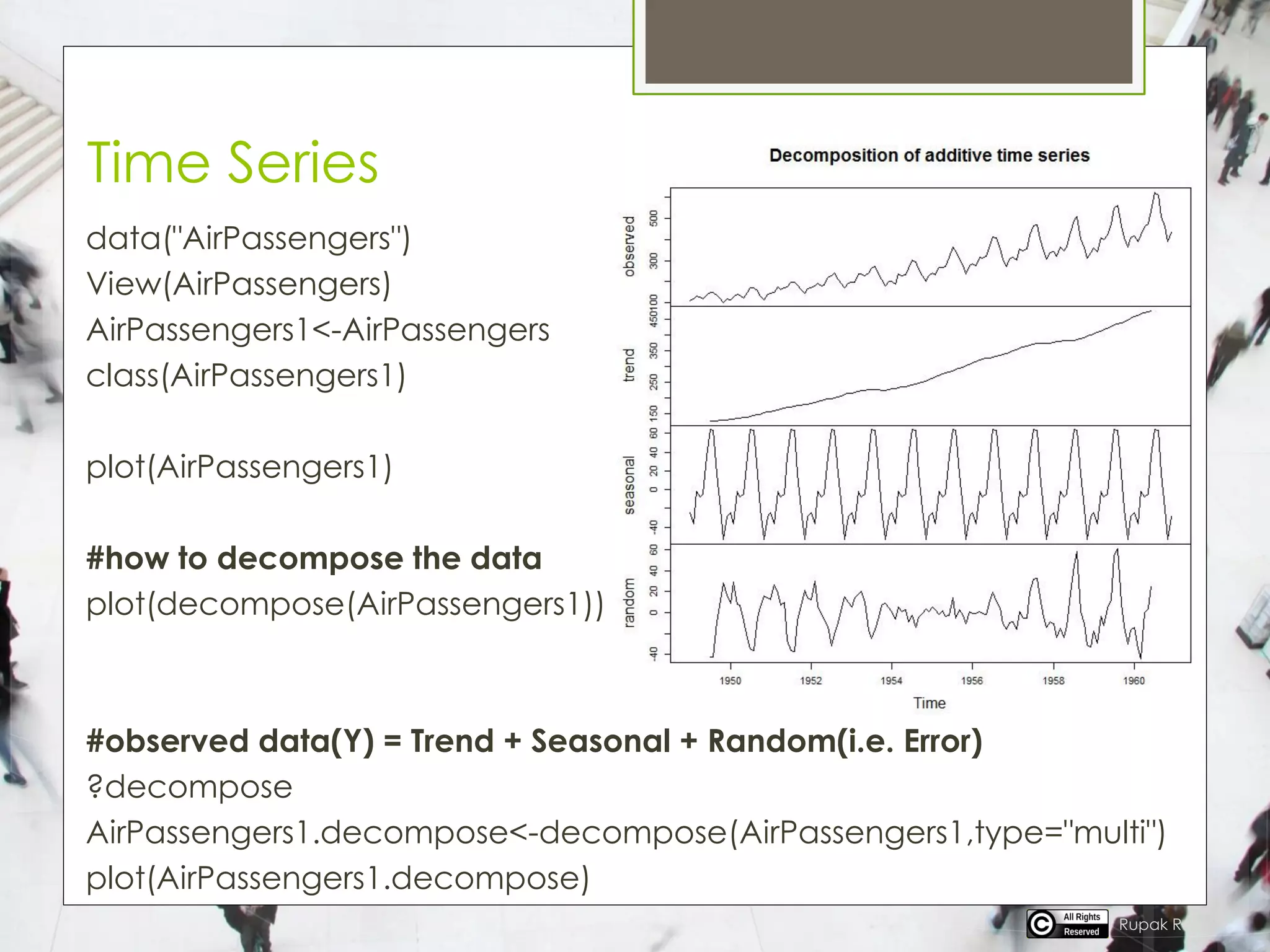
The document discusses time series analysis, which involves studying data collected over time to identify patterns and trends. It outlines the main components of time series data, including trend, seasonal, irregular, and cyclic components, and provides examples of applications in fields like health and finance. Additionally, the document mentions methods for smoothing time series data, such as simple moving averages and exponential moving averages.

1. Machine
Learning - VI
Time Series

2. Time Series
 Time series: a series of values of a quantity obtained at successive
times, often with equal intervals between them, in simple words data
is in a series of particular time periods or intervals.
 And the analysis of Time series is a statistical technique that deals with
time series data, or trend analysis.
Example: health applications which require continuous monitoring ,
forecast sales over revenue, stock exchange, weather etc.
It is basically used to understand the systematic pattern of the
underlying structure that produces the observations/events.
Understanding the systematic pattern of time series data helps us to
forecast and develop predictive control measures for the next time
series event.
Rupak Roy

3. Time Series Components
In General a time series consists of 3 components
• Trend Component: It is the main component of the time series that
moves up or down in a reasonably predictable pattern.
• Seasonal Component: that repeats over a specific period such as a
day, week, month, season, etc due to seasonal factors like sales of
ice- cream is higher in summer than other months.
• Irregular Component: These are sudden changes occurring which
are unlikely to be repeated which cannot be explained by trends,
seasonal or cyclic movements. These variations are sometimes called
residual or random component.
• Cyclic Component: It spans like more than one year like one
complete period = 1cycle. This oscillatory movement are mostly
observed in economical data.
Rupak Roy

4. Time Series
data("AirPassengers")
View(AirPassengers)
AirPassengers1<-AirPassengers
class(AirPassengers1)
plot(AirPassengers1)
#how to decompose the data
plot(decompose(AirPassengers1))
#observed data(Y) = Trend + Seasonal + Random(i.e. Error)
?decompose
AirPassengers1.decompose<-decompose(AirPassengers1,type="multi")
plot(AirPassengers1.decompose)
Rupak Roy

5. Time Series
#To see the components separately
AirPassengers1.trend<-AirPassengers1.decompose$trend
AirPassengers1.seasonal<-AirPassengers1.decompose$seasonal
#seasonal
#trend
AirPassengers1.seasonal
AirPassengers1.trend
#To plot season and trend together
ts.plot(cbind(AirPassengers1.trend,AirPassengers1.trend*AirPassengers1.
seasonal))
Rupak Roy

6. Next
Data smoothening methods to reduce noise for time series by Simple
Moving Averages and Exponential Moving Averages.
Rupak Roy