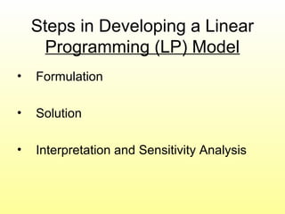
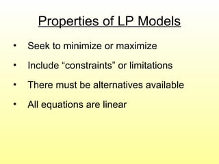
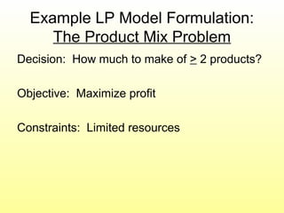
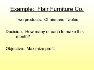
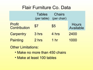
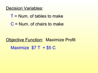
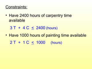
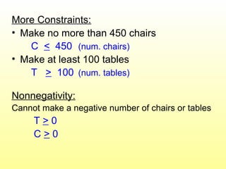
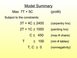
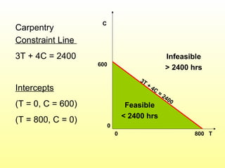
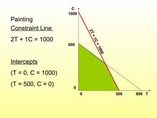
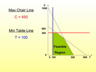
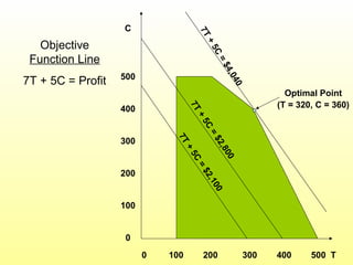
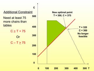
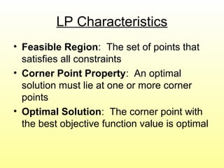
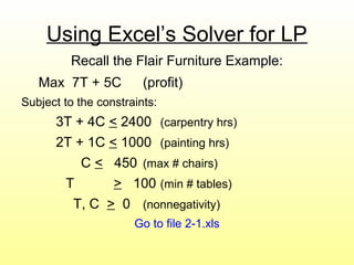
Chapter 2
Linear Programming Models:
Graphical and Computer Methods
Steps in Developing a Linear
Programming (LP) Model
• Formulation
• Solution
• Interpretation and Sensitivity Analysis
Properties of LP Models
• Seek to minimize or maximize
• Include “constraints” or limitations
• There must be alternatives available
• All equations are linear
Example LP Model Formulation:
The Product Mix Problem
Decision: How much to make of > 2 products?
Objective: Maximize profit
Constraints: Limited resources
Example: Flair Furniture Co.
Two products: Chairs and Tables
Decision: How many of each to make this
month?
Objective: Maximize profit
Flair Furniture Co. Data
Tables
(per table)
Chairs
(per chair)
Hours
Available
Profit
Contribution $7 $5
Carpentry 3 hrs 4 hrs 2400
Painting 2 hrs 1 hr 1000
Other Limitations:
• Make no more than 450 chairs
• Make at least 100 tables
Decision Variables:
T = Num. of tables to make
C = Num. of chairs to make
Objective Function: Maximize Profit
Maximize $7 T + $5 C
Constraints:
• Have 2400 hours of carpentry time
available
3 T + 4 C < 2400 (hours)
• Have 1000 hours of painting time available
2 T + 1 C < 1000 (hours)
More Constraints:
• Make no more than 450 chairs
C < 450 (num. chairs)
• Make at least 100 tables
T > 100 (num. tables)
Nonnegativity:
Cannot make a negative number of chairs or tables
T > 0
C > 0
Model Summary
Max 7T + 5C (profit)
Subject to the constraints:
3T + 4C < 2400 (carpentry hrs)
2T + 1C < 1000 (painting hrs)
C < 450 (max # chairs)
T > 100 (min # tables)
T, C > 0 (nonnegativity)
Graphical Solution
• Graphing an LP model helps provide
insight into LP models and their solutions.
• While this can only be done in two
dimensions, the same properties apply to
all LP models and solutions.
Carpentry
Constraint Line
3T + 4C = 2400
Intercepts
(T = 0, C = 600)
(T = 800, C = 0)
0 800 T
C
600
0
Feasible
< 2400 hrs
Infeasible
> 2400 hrs
3T
+
4C
=
2400
Painting
Constraint Line
2T + 1C = 1000
Intercepts
(T = 0, C = 1000)
(T = 500, C = 0)
0 500 800 T
C
1000
600
0 2T+1C=1000
0 100 500 800 T
C
1000
600
450
0
Max Chair Line
C = 450
Min Table Line
T = 100
Feasible
Region
0 100 200 300 400 500 T
C
500
400
300
200
100
0
Objective
Function Line
7T + 5C = Profit
7T
+
5C
=
$2,100
7T+5C
=$4,040
Optimal Point
(T = 320, C = 360)
7T
+5C
=$2,800
0 100 200 300 400 500 T
C
500
400
300
200
100
0
Additional Constraint
Need at least 75
more chairs than
tables
C > T + 75
Or
C – T > 75
T = 320
C = 360
No longer
feasible
New optimal point
T = 300, C = 375
LP Characteristics
• Feasible Region: The set of points that
satisfies all constraints
• Corner Point Property: An optimal
solution must lie at one or more corner
points
• Optimal Solution: The corner point with
the best objective function value is optimal
Special Situation in LP
• Redundant Constraints - do not affect
the feasible region
Example: x < 10
x < 12
The second constraint is redundant
because it is less restrictive.
Special Situation in LP
• Infeasibility – when no feasible solution
exists (there is no feasible region)
Example: x < 10
x > 15
Special Situation in LP
• Alternate Optimal Solutions – when
there is more than one optimal solution
Max 2T + 2C
Subject to:
T + C < 10
T < 5
C < 6
T, C > 0
0 5 10 T
C
10
6
0
2T
+
2C
=
20
All points on
Red segment
are optimal
Special Situation in LP
• Unbounded Solutions – when nothing
prevents the solution from becoming
infinitely large
Max 2T + 2C
Subject to:
2T + 3C > 6
T, C > 0
0 1 2 3 T
C
2
1
0
Direction
of solution
Using Excel’s Solver for LP
Recall the Flair Furniture Example:
Max 7T + 5C (profit)
Subject to the constraints:
3T + 4C < 2400 (carpentry hrs)
2T + 1C < 1000 (painting hrs)
C < 450 (max # chairs)
T > 100 (min # tables)
T, C > 0 (nonnegativity)
Go to file 2-1.xls

Lpp 2.1202.ppts

  • 1.
    Chapter 2 Linear ProgrammingModels: Graphical and Computer Methods
  • 2.
    Steps in Developinga Linear Programming (LP) Model • Formulation • Solution • Interpretation and Sensitivity Analysis
  • 3.
    Properties of LPModels • Seek to minimize or maximize • Include “constraints” or limitations • There must be alternatives available • All equations are linear
  • 4.
    Example LP ModelFormulation: The Product Mix Problem Decision: How much to make of > 2 products? Objective: Maximize profit Constraints: Limited resources
  • 5.
    Example: Flair FurnitureCo. Two products: Chairs and Tables Decision: How many of each to make this month? Objective: Maximize profit
  • 6.
    Flair Furniture Co.Data Tables (per table) Chairs (per chair) Hours Available Profit Contribution $7 $5 Carpentry 3 hrs 4 hrs 2400 Painting 2 hrs 1 hr 1000 Other Limitations: • Make no more than 450 chairs • Make at least 100 tables
  • 7.
    Decision Variables: T =Num. of tables to make C = Num. of chairs to make Objective Function: Maximize Profit Maximize $7 T + $5 C
  • 8.
    Constraints: • Have 2400hours of carpentry time available 3 T + 4 C < 2400 (hours) • Have 1000 hours of painting time available 2 T + 1 C < 1000 (hours)
  • 9.
    More Constraints: • Makeno more than 450 chairs C < 450 (num. chairs) • Make at least 100 tables T > 100 (num. tables) Nonnegativity: Cannot make a negative number of chairs or tables T > 0 C > 0
  • 10.
    Model Summary Max 7T+ 5C (profit) Subject to the constraints: 3T + 4C < 2400 (carpentry hrs) 2T + 1C < 1000 (painting hrs) C < 450 (max # chairs) T > 100 (min # tables) T, C > 0 (nonnegativity)
  • 11.
    Graphical Solution • Graphingan LP model helps provide insight into LP models and their solutions. • While this can only be done in two dimensions, the same properties apply to all LP models and solutions.
  • 12.
    Carpentry Constraint Line 3T +4C = 2400 Intercepts (T = 0, C = 600) (T = 800, C = 0) 0 800 T C 600 0 Feasible < 2400 hrs Infeasible > 2400 hrs 3T + 4C = 2400
  • 13.
    Painting Constraint Line 2T +1C = 1000 Intercepts (T = 0, C = 1000) (T = 500, C = 0) 0 500 800 T C 1000 600 0 2T+1C=1000
  • 14.
    0 100 500800 T C 1000 600 450 0 Max Chair Line C = 450 Min Table Line T = 100 Feasible Region
  • 15.
    0 100 200300 400 500 T C 500 400 300 200 100 0 Objective Function Line 7T + 5C = Profit 7T + 5C = $2,100 7T+5C =$4,040 Optimal Point (T = 320, C = 360) 7T +5C =$2,800
  • 16.
    0 100 200300 400 500 T C 500 400 300 200 100 0 Additional Constraint Need at least 75 more chairs than tables C > T + 75 Or C – T > 75 T = 320 C = 360 No longer feasible New optimal point T = 300, C = 375
  • 17.
    LP Characteristics • FeasibleRegion: The set of points that satisfies all constraints • Corner Point Property: An optimal solution must lie at one or more corner points • Optimal Solution: The corner point with the best objective function value is optimal
  • 18.
    Special Situation inLP • Redundant Constraints - do not affect the feasible region Example: x < 10 x < 12 The second constraint is redundant because it is less restrictive.
  • 19.
    Special Situation inLP • Infeasibility – when no feasible solution exists (there is no feasible region) Example: x < 10 x > 15
  • 20.
    Special Situation inLP • Alternate Optimal Solutions – when there is more than one optimal solution Max 2T + 2C Subject to: T + C < 10 T < 5 C < 6 T, C > 0 0 5 10 T C 10 6 0 2T + 2C = 20 All points on Red segment are optimal
  • 21.
    Special Situation inLP • Unbounded Solutions – when nothing prevents the solution from becoming infinitely large Max 2T + 2C Subject to: 2T + 3C > 6 T, C > 0 0 1 2 3 T C 2 1 0 Direction of solution
  • 22.
    Using Excel’s Solverfor LP Recall the Flair Furniture Example: Max 7T + 5C (profit) Subject to the constraints: 3T + 4C < 2400 (carpentry hrs) 2T + 1C < 1000 (painting hrs) C < 450 (max # chairs) T > 100 (min # tables) T, C > 0 (nonnegativity) Go to file 2-1.xls