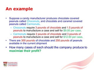
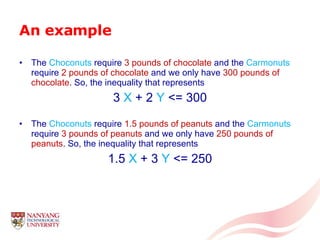
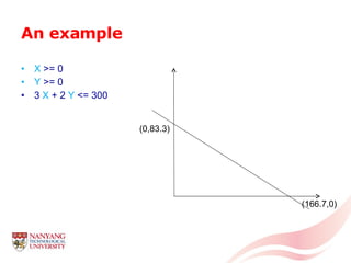
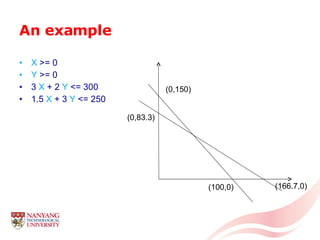
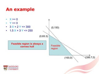
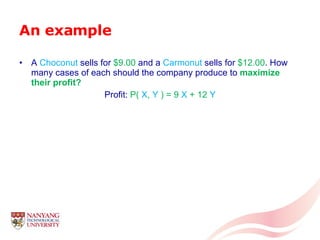
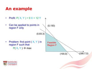
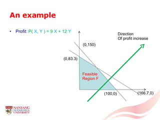
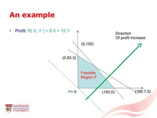
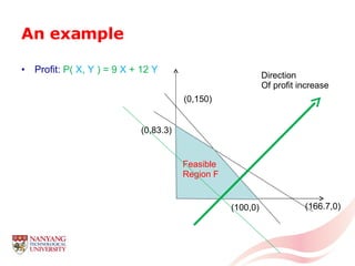
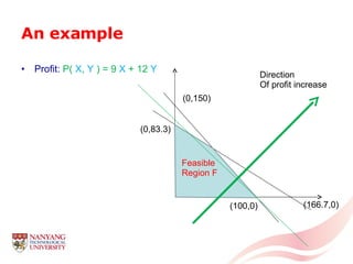
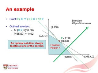
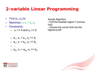
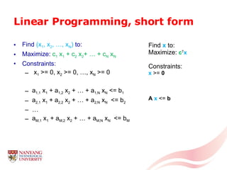
The document introduces linear programming through an example of a candy manufacturer that must determine how many cases of two candy products to make to maximize profit given constraints on available ingredients. It defines variables and constraints, graphs the feasible region, determines the optimal solution that maximizes profit, and discusses how linear programming can be applied to problems with multiple variables and constraints.

1. An Introduction to Linear Programming Pham Minh Tri Ph.D. Candidate and Project Officer School of Computer Engineering 18 Jan 2008 presented by

2. An example Suppose a candy manufacturer produces chocolate covered peanuts called Choconuts , and chocolate and caramel covered peanuts called Carmonuts . Choconuts require 3 pounds of chocolate and 1.5 pounds of peanuts to manufacture a case and sell for $9.00 per case . Carmonuts require 2 pounds of chocolate and 3 pounds of peanuts to manufacture a case and sell for $12.00 per case . There are 300 pounds of chocolate and 250 pounds of peanuts available in the current shipment How many cases of each should the company produce to maximize their profit?

3. An example First, let’s define our variables: X = number of cases of Choconuts to produce Y = number of cases of Carmonuts to produceSuppose a candy

4. An example The Choconuts require 3 pounds of chocolate and the Carmonuts require 2 pounds of chocolate and we only have 300 pounds of chocolate . So, the inequality that represents 3 X + 2 Y <= 300 The Choconuts require 1.5 pounds of peanuts and the Carmonuts require 3 pounds of peanuts and we only have 250 pounds of peanuts . So, the inequality that represents 1.5 X + 3 Y <= 250

5. An example Now, since we cannot produce a negative amount of either candy, we also have these constraints: X >= 0 Y >= 0 Let’s graph these inequalities;

6. An example

7. An example X >= 0

8. An example X >= 0 Y >= 0

9. An example X >= 0 Y >= 0 3 X + 2 Y <= 300 (0,83.3) (166.7,0)

10. An example X >= 0 Y >= 0 3 X + 2 Y <= 300 1.5 X + 3 Y <= 250 (0,83.3) (100,0) (0,150) (166.7,0)

11. An example X >= 0 Y >= 0 3 X + 2 Y <= 300 1.5 X + 3 Y <= 250 (0,83.3) (100,0) (0,150) (166.7,0) Feasible region Feasible region is always a convex hull

12. An example A Choconut sells for $9.00 and a Carmonut sells for $12.00 . How many cases of each should the company produce to maximize their profit? Profit: P( X , Y ) = 9 X + 12 Y

13. An example Profit: P( X , Y ) = 9 X + 12 Y Can be applied to points in region F only Problem: find point ( X , Y ) in region F such that P ( X , Y )  max (0,83.3) (100,0) (0,150) (166.7,0) Feasible Region F

14. An example Profit: P( X , Y ) = 9 X + 12 Y (0,83.3) (100,0) (0,150) (166.7,0) Feasible Region F Direction Of profit increase

15. An example Profit: P( X , Y ) = 9 X + 12 Y (0,83.3) (100,0) (0,150) (166.7,0) Feasible Region F Direction Of profit increase P = 0

16. An example Profit: P( X , Y ) = 9 X + 12 Y (0,83.3) (100,0) (0,150) (166.7,0) Feasible Region F Direction Of profit increase

17. An example Profit: P( X , Y ) = 9 X + 12 Y (0,83.3) (100,0) (0,150) (166.7,0) Feasible Region F Direction Of profit increase

18. An example Profit: P( X , Y ) = 9 X + 12 Y (0,83.3) (100,0) (0,150) (166.7,0) Feasible Region F Direction Of profit increase

19. An example Profit: P( X , Y ) = 9 X + 12 Y (0,83.3) (100,0) (0,150) (166.7,0) Feasible Region F Direction Of profit increase

20. An example Profit: P( X , Y ) = 9 X + 12 Y Optimal solution: At ( X , Y )=(66,50) P(66,50) = 1192 (0,83.3) (100,0) (0,150) (166.7,0) Feasible Region F Direction Of profit increase P = 1192 (66,50) An optimal solution, always locates at one of the corners

21. 2-variable Linear Programming Find (x 1 ,x 2 ) to: Maximize: c 1 x 1 + c 2 x 2 Constraints: x 1 >= 0 and x 2 >= 0 a 1,1 x 1 + a 1,2 x 2 <= b 1 a 2,1 x 1 + a 2,2 x 2 <= b 2 … a M,1 x 1 + a M,2 x 2 <= b M Simple Algorithm: - Find the feasible region F (convex hull) - Choose the corner that has the highest profit

22. What about over 2 variables? Same idea, except that feasible region F lives in a higher dimensional space: 2-variable linear programming: F = 2D convex hull 3-variable linear programming: F = 3D convex hull 4-variable linear programming: F = 4D convex hull etc

23. Linear Programming in general Find (x 1 , x 2 , …, x N ) to: Maximize: c 1 x 1 + c 2 x 2 + … + c N x N Constraints: x 1 >= 0, x 2 >= 0, …, x N >= 0 a 1,1 x 1 + a 1,2 x 2 + … + a 1,N x N <= b 1 a 2,1 x 1 + a 2,2 x 2 + … + a 2,N x N <= b 2 … a M,1 x 1 + a M,2 x 2 + … + a M,N x N <= b M

24. Linear Programming, short form Find (x 1 , x 2 , …, x N ) to: Maximize: c 1 x 1 + c 2 x 2 + … + c N x N Constraints: x 1 >= 0, x 2 >= 0, …, x N >= 0 a 1,1 x 1 + a 1,2 x 2 + … + a 1,N x N <= b 1 a 2,1 x 1 + a 2,2 x 2 + … + a 2,N x N <= b 2 … a M,1 x 1 + a M,2 x 2 + … + a M,N x N <= b M Find x to: Maximize: c T x Constraints: x >= 0 A x <= b

25. Linear Programming If we multiply each constraint with a non-negative number, and sum them up: y 1 >= 0, y 2 >= 0, …, y M >= 0 y 1 (a 1,1 x 1 + a 1,2 x 2 + … + a 1,N x N ) <= y 1 b 1 y 2 (a 2,1 x 1 + a 2,2 x 2 + … + a 2,N x N ) <= y 2 b 2 … y M (a M,1 x 1 + a M,2 x 2 + … + a M,N x N )<= y M b M The equation y T A x <= y T b holds for every non-negative vector y y T A x <= y T b

26. Linear Programming Let us limit the choices for y further. Suppose we are interested in only y such that: y 1 >= 0, y 2 >= 0, …, y M >= 0 y 1 a 1,1 + y 2 a 2,1 + … + y M a M,1 >= c 1 y 1 a 1,2 + y 2 a 2,2 + … + y M a M,2 >= c 2 … y 1 a 1,N + y 2 a 2,N + … + y M a M,N >= c N This leads to: y T A x >= c T x y T A >= c T Let’s call this feasible region G for y

27. Linear Programming - Duality Hence, we have this nice property: For all: vector x in F, and y in G: c T x <= y T A x <= y T b This leads to the following Duality theorem;

28. Linear Programming - Duality The following two problems are equivalent: Primal problem: Maximize c T x Subject to A x <= b , x >= 0 Dual problem: Minimize b T y Subject to A T y >= c , y >= 0

29. Linear Programming - Duality Furthermore, at the optimal solution, we have the following complementary slackness theorem : (no proof, sorry!) y i (a i,1 x 1 + a i,2 x 2 + … + a i,N x N -b i ) = 0 x i (a 1,i y 1 + a 2,i y 2 + … + a M,i y N - c i ) = 0 Using this duality, we can convert a problem with many variables but a few constraints (hard to solve) into a problem of multiple constraints with a few variables (easy to solve).

30. Another example A burglar breaks into a bank’s storeroom. He notices that the items in the room are in one of ten different types. Each item type has its own value , volume , and weight . The items are homogeneous and can be broken into pieces while still preserving their values. There are so many valuable items for each type that he cannot even count. The burglar brings along with him a small bag, which can help him carry at most M kilograms with maximum volume of N meter cubed . Help him decide how many items per type he should steal to maximize the total value .

31. Another example Suppose the i-th item type has value a i , weight w i , and volume v i Let’s define our variables: x 1 = number of items of type 1 x 2 = number of items of type 2 … x 10 = number of items of type 10

32. Another example There is no way the number of items is negative, therefore: x 1 >= 0 x 2 >= 0 … x 10 >= 0 Weight constraint: w 1 x 1 + w 2 x 2 + … + w 10 x 10 <= M Volume constraint: v 1 x 1 + v 2 x 2 + … + v 10 x 10 <= N Objective function: a 1 x 1 + a 2 x 2 + … + a 10 x 10

33. Another example The primal problem has 10 variables and 2 constraints. To solve it, we need to work with a 10D convex hull!!! If we convert into the dual problem, we have 2 variables and 10 constraints as follows: Minimize: M y 1 + N y 2 Subject to: y 1 >= 0, y 2 >= 0 w 1 y 1 + v 1 y 2 >= a 1 w 2 y 1 + v 2 y 2 >= a 2 … w 10 y 1 + v 10 y 2 >= a 10

34. Another example Once we have found optimal y =( y 1 , y 2 ), we can use the complementary slackness theorem to find x =( x 1 , x 2 , …, x 10 ): y 1 (w 1 x 1 + w 2 x 2 + … + w 10 x 10 -M) = 0 y 2 (v 1 x 1 + v 2 x 2 + … + v 10 x 10 -N) = 0 x i (w i y 1 + v i y 2 - a i ) = 0 for i = 1 to 10 Thus: In the last 10 equations, if w i y 1 + v i y 2 > a i then x i must be 0 The remaining x i ’s can be found by solving the remaining system of linear equations.