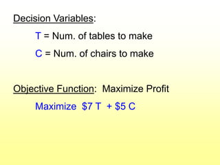
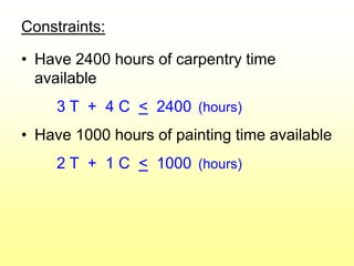
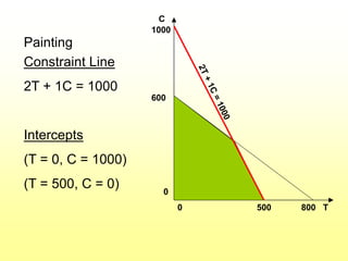
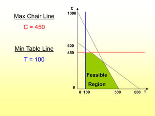
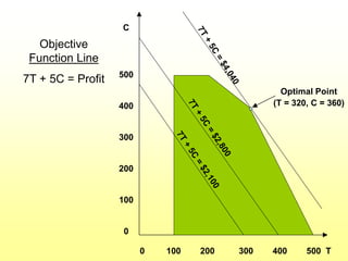
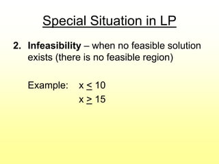
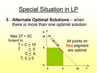
Chapter 2 discusses linear programming (LP) models, focusing on their formulation, solution, and interpretation. It illustrates the product mix problem using the example of Flair Furniture Co., detailing constraints, the objective function, and graphical solutions. Additionally, the chapter covers special situations in LP, such as redundant constraints, infeasibility, alternate optimal solutions, and unbounded solutions.

1. Chapter 2
Linear Programming Models:
Graphical and Computer Methods
© 2007 Pearson Education

2. Steps in Developing a Linear
Programming (LP) Model
1) Formulation
2) Solution
3) Interpretation and Sensitivity Analysis

3. Properties of LP Models
1) Seek to minimize or maximize
2) Include “constraints” or limitations
3) There must be alternatives available
4) All equations are linear

4. Example LP Model Formulation:
The Product Mix Problem
Decision: How much to make of > 2 products?
Objective: Maximize profit
Constraints: Limited resources

5. Example: Flair Furniture Co.
Two products: Chairs and Tables
Decision: How many of each to make this
month?
Objective: Maximize profit

6. Flair Furniture Co. Data
Tables
(per table)
Chairs
(per chair)
Hours
Available
Profit
Contribution
$7 $5
Carpentry 3 hrs 4 hrs 2400
Painting 2 hrs 1 hr 1000
Other Limitations:
• Make no more than 450 chairs
• Make at least 100 tables

7. Decision Variables:
T = Num. of tables to make
C = Num. of chairs to make
Objective Function: Maximize Profit
Maximize $7 T + $5 C

8. Constraints:
• Have 2400 hours of carpentry time
available
3 T + 4 C < 2400 (hours)
• Have 1000 hours of painting time available
2 T + 1 C < 1000 (hours)

9. More Constraints:
• Make no more than 450 chairs
C < 450 (num. chairs)
• Make at least 100 tables
T > 100 (num. tables)
Nonnegativity:
Cannot make a negative number of chairs or tables
T > 0
C > 0

10. Model Summary
Max 7T + 5C (profit)
Subject to the constraints:
3T + 4C < 2400 (carpentry hrs)
2T + 1C < 1000 (painting hrs)
C < 450 (max # chairs)
T > 100 (min # tables)
T, C > 0 (nonnegativity)

11. Graphical Solution
• Graphing an LP model helps provide
insight into LP models and their solutions.
• While this can only be done in two
dimensions, the same properties apply to
all LP models and solutions.

12. Carpentry
Constraint Line
3T + 4C = 2400
Intercepts
(T = 0, C = 600)
(T = 800, C = 0)
0 800 T
C
600
0
Feasible
< 2400 hrs
Infeasible
> 2400 hrs

13. Painting
Constraint Line
2T + 1C = 1000
Intercepts
(T = 0, C = 1000)
(T = 500, C = 0)
0 500 800 T
C
1000
600
0

14. 0 100 500 800 T
C
1000
600
450
0
Max Chair Line
C = 450
Min Table Line
T = 100
Feasible
Region

15. 0 100 200 300 400 500 T
C
500
400
300
200
100
0
Objective
Function Line
7T + 5C = Profit
Optimal Point
(T = 320, C = 360)

16. 0 100 200 300 400 500 T
C
500
400
300
200
100
0
Additional Constraint
Need at least 75
more chairs than
tables
C > T + 75
Or
C – T > 75
T = 320
C = 360
No longer
feasible
New optimal point
T = 300, C = 375

17. LP Characteristics
• Feasible Region: The set of points that
satisfies all constraints
• Corner Point Property: An optimal
solution must lie at one or more corner
points
• Optimal Solution: The corner point with
the best objective function value is optimal

18. Special Situation in LP
1. Redundant Constraints - do not affect
the feasible region
Example: x < 10
x < 12
The second constraint is redundant
because it is less restrictive.

19. Special Situation in LP
2. Infeasibility – when no feasible solution
exists (there is no feasible region)
Example: x < 10
x > 15

20. Special Situation in LP
3. Alternate Optimal Solutions – when
there is more than one optimal solution
Max 2T + 2C
Subject to:
T + C < 10
T < 5
C < 6
T, C > 0
0 5 10 T
C
10
6
0
All points on
Red segment
are optimal

21. Special Situation in LP
4. Unbounded Solutions – when nothing
prevents the solution from becoming
infinitely large
Max 2T + 2C
Subject to:
2T + 3C > 6
T, C > 0
0 1 2 3 T
C
2
1
0

22. Using Excel’s Solver for LP
Recall the Flair Furniture Example:
Max 7T + 5C (profit)
Subject to the constraints:
3T + 4C < 2400 (carpentry hrs)
2T + 1C < 1000 (painting hrs)
C < 450 (max # chairs)
T > 100 (min # tables)
T, C > 0 (nonnegativity)
Go to file 2-1.xls