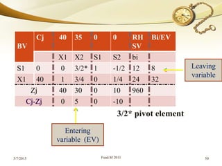
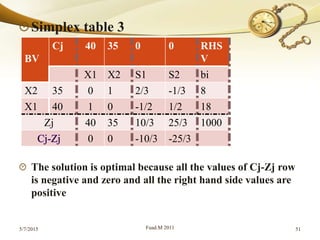
The document discusses linear programming (LP) and its solution methods. It provides an overview of LP, describing it as a technique for optimization problems where the objective function and constraints are expressed as linear equations. Two common solution methods are then discussed: graphical and simplex. The graphical method involves plotting the constraints on a graph and finding the optimal solution at the corner point of the feasible region. The simplex method is an iterative algebraic approach that moves between basic feasible solutions to optimize the objective function.

1. Operations Research
by
FUAD MUSTEFA
5/7/2015 1Fuad.M 2011
Linear Programming
CHAPTER
TWO

2. Linear Programming is that branch of mathematical programming
which is designed to solve optimization problems where all the
constraints as will as the objectives are expressed as Linear function .
Linear Programming is a technique for making decisions under
certainty i.e.; when all the courses of actions available to an
organization are known & the objective of the firm along with its
constraints are quantified.
LP is the analysis of problems in which a Linear function of a number
of variables is to be optimized (maximized or minimized) when whose
variables are subject to a number of constraints in the mathematical
inequalities.
5/7/2015 Fuad.M 2011 2

3. From the above definitions, it is clear that:
LP is an optimization technique
It deals with the problem of allocation of
scarce sources
It generates solutions based on the feature
and characteristics of the actual problem or
situation.
5/7/2015 Fuad.M 2011 3

4. Product-mix problems Investment planning problems
Blending strategy formulations
and
Marketing & Distribution
management.
LP has been highly
successful in solving
the following types of
problems :
5/7/2015 Fuad.M 2011 4

5. All LPP have the following
properties in common .
• The objective is always the same
• Presence of constraints which limit the extent to which the
objective can be pursued/achieved.
• Availability of alternatives
• The objectives and constraints can be expressed in the form of
linear relation.
5/7/2015 Fuad.M 2011 5

6. Decision or Activity Variables & Their Inter-Relationship
Finite Objective Functions
Limited Factors/Constraints
Presence of Different Alternatives
Non-Negativity Restrictions
Linearity Criterion
Additive
Mutually Exclusive Criterion
Divisibility
Certainty
Finiteness.
5/7/2015 Fuad.M 2011 6

7. Military Applications
Agriculture
Environmental Protection.
Facilities Location
Product-Mix
Production
Mixing or Blending
Transportation & Trans-
Shipment
Portfolio Selection
Profit Planning & Contract.
Traveling Salesmen
Problem
Media Selection/Evaluation
Staffing
Job Analysis
Wages and Salary
Administration.
5/7/2015 Fuad.M 2011 7

8. Steps in Formulating a LP Model
Step I Identification of the decision variables
Step II Identification of the constraints
Step III formulate the objective function
Step IV formulate as LPP
5/7/2015 Fuad.M 2011 8

9. 3F furniture Ltd. manufactures two products, tables & chair. Both
the products have to be processed through two machines Ml & M2
the total machine-hours available are: 200 hours of M1 and 400
hours of M2 respectively. Time in hours required for producing a
chair and a table on both the machines is as follows:
5/7/2015 Fuad.M 2011 9
Machine Table Chair
M1 7 4
M2 5 5
Profit from the Sale of table is Birr 40 and that of a chair is Birr 30.
Required: formulate the LP Problem (LPP)?

10. Step I Identification of the decision variables. Let x1 = Number of
tables produced and X2 = Number of Chairs produced
5/7/2015 Fuad.M 2011 10
Step II List down all the constraints :
A. Total time on machine M1 cannot exceed 200 hour
∴ 7X1+4X2≤200 and
B. Total time on machine M2 cannot exceed 400 hour
∴ 5X1+5X2≤400
Step III. The objective function for maximizing the profit is
given by.
Minimize Z= 40X1+30X2
Presenting the problem as LPP
Minimize Z= 40X1+30X2
subject to: 7X1+4X2≤200
5X1+5X2≤400 X1&X2≥0

11. Alpha Limited company produces & sells 2 different products
under the brand name black & white. The profit per unit on these
products is Birr 50 & Birr 40 respectively. Both black & white
employ the same manufacturing process which has a fixed total
capacity of 50,000 man-hour. As per the estimates of the
marketing research department of Alpha Limited, there is a market
demand for maximum 8,000 units of Black & 10,000 units of
white. Subject to the overall demand, the products can be sold in
any possible combination. If it takes 3 hours to produce one unit
of black & 2 hours to produce one unit of white. Formulate the
above problem as a linear programming model?
5/7/2015 Fuad.M 2011 11

12. 3. An agriculturalist has a 125 acre farm. He produce onion,
tomato and potato. What ever he rises is fully sold in the
market. He gets Birr 5 for onion per kg, Birr 4 for tomato per
kg and Birr 5 for potato per kg. The average per acre yield is
1500kg of onion, 1800kg of tomato and 1200kg of potato. To
produce each 100kg of onion and tomato and 80kg potato, a
sum of Birr 12.5 has to be used for fertilizer. Labor required
for each acre to rise the crop is 6 man days for onion and
potato each and 5 man-days for tomato. A total of 500 man-
days of labor at a rate of Birr 40 per man-day are available.
Formulate this as LP model to maximize the agriculturist’s
total profit.
5/7/2015 Fuad.M 2011 12

13. There are two types of finding a
solution for Linear programming
problems.
• Graphic solution and
• Simplex solution
5/7/2015 Fuad.M 2011 13

14. The graphic solution procedure is one of the methods of
solving two variable linear programming problems.
Steps in graphic solution method
Step I Defining the problem
Step II Plot the constraints Graphically
Step III Locate the solution space: Solution space or the
feasible region is the graphical area which satisfies all the
constraints at the same time. Such a solution point (x, y)
always occurs at the corner Points of the feasible Region the
feasible region is determined as follows:
5/7/2015 Fuad.M 2011 14

15. 1. For "greater than" & "greater than or equal to" constraints,
the feasible region or the solution space is the area that lays
above the constraint lines.
2. For" Less Then" &" Less than or equal to" constraint, the
feasible region or the solution space is the area that lays
below the constraint lines.
Step IV Selecting the graphic solution technique
There are two graphic techniques to find solution;
a. Corner Point Method and
b. Iso-profit (or Iso-cost) method may be used
5/7/2015 Fuad.M 2011 15

16. Since the solution point (x, y) always occurs at the corner
point of the feasible or solution space, identify each of the
extreme points or corner points of the feasible region by the
method of simultaneous equations.
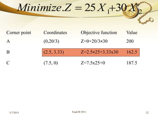
By putting the value of the corner point's co-ordinates [e.g. (2,
3)] into the objective function, calculate the profit (or the cost)
at each of the corner points.
In a Maximize problem, the optimal solution occurs at that
corner point which gives the highest profit. In a minimization
problem, the optimal solution occurs at that corner point which
gives the lowest profit.
5/7/2015 Fuad.M 2011 16

17. XYZ Ltd. Co. Wishes to purchase a maximum of 3600 units
of two types of product, A & B are available in the market.
Product A occupies a space of 3 cubic feet & cost Birr 9
whereas B occupies a space of 1 cubic feet & cost Birr 13
per unit. The budgetary constraints of the company do not
allow spending more than Birr 39,000. The total availability
of space in the company's god own is 6000 cubic feet. Profit
margin of both the product A & B is Birr 3 & Birr 4
respectively. Formulate the above problem as a linear
programming model and solve it by using graphical method.
You are required to ascertain the best possible combination
of purchase of A & B so that the total profits are maximized.
5/7/2015 Fuad.M 2011 17

18. Graphic solution EG. Cont…
5/7/2015 Fuad.M 2011
Number of unites o A
Y
C
6000
3600
3000
2000 3600 3900/9
X
NumberofunitesofB
A1
(0, 0)
B(1300,2100)
3X+Y≤6000 (Storage area constraint)
X+Y≤3600(Maximum unites constraint)
9X+13Y≤3900(Budgetary constraint)
o
Feasible
region

19. 5/7/2015 Fuad.M 2011 19
Corner point Coordinates Objective function Value
O (0,0) Z=0+0 0
A (0,3000) Z=0+4x3000 12,000
B (1300,2100) Z=3x1300 + 4 x2100 12,300
C (2000,0) Z=3 x 2000 + 0 6000

20. 2. Suppose that a machine shop has two different types of machines;
machine 1 and machine 2, which can be used to make a single
product .These machine vary in the amount of product produced per
hour, in the amount of labor used and in the cost of operation.
Assume that at least a certain amount of product must be produced
and we would like to utilize at least the regular labor force. How
much should we utilize in each machine in order to utilize total
costs and still meets the requirement? The resource used, the cost
and the required hour is given in the following table.
20
Machine 1
(X)
Machine 2
(Y)
Minimum required hours
Product produced/hr 20 15 100
Labor/hr 2 3 15
Operation Cost Birr25 Birr30

21. 5/7/2015 Fuad.M 2011 21
B (2.5, 3.33)
A (0, 20/3)
C (7.5, 0)
Y
5
X2 =0
Y=0
Feasible Region
2X1 + 3X2 ≥ 15
20X+15Y≥100
5
X

22. 5/7/2015 Fuad.M 2011 22
Corner point Coordinates Objective function Value
A
B
C
(0,20/3)
(2.5, 3.33)
(7.5, 0)
Z=0+20/3×30
Z=2.5×25+3.33x30
Z=7.5x25+0
200
162.5
187.5
21 3025. XXZMinimize 

23. The following are the major special cases in graphics solution
a. Alternative Optima
b. Infeasible Solution
c. Unbounded solution
5/7/2015 Fuad.M 2011 23
a. Alternative Optimal solution
When the objective function is parallel to a binding constraint; (a
constraint that is satisfied in the equality sense by the optimal
solution), the objective function will assume the same optimal
value at more than one solution point, for this reason they are
called alternative optima.

24. 5/7/2015 Fuad.M 2011 24

25. Example :
The information given below is for the products A and B.
5/7/2015 Fuad.M 2011 25
Machine hours per week Maximum available
Department Product A Product B per week
Cutting 3 6 900
Assembly 1 1 200
Profit per unit Birr 8 Birr 16
Assume that the company has a marketing constraint on selling
products B and therefore it can sale a maximum of 125 units of this
product.
Required:
a. Formulate the LPP of this problem?
b. Find the optimal solution?

26. 5/7/2015 Fuad.M 2011 26
The LPP Model of the problem is:
0,
125
200
90063
:
168.
21
2
21
21
21





XX
X
XX
XX
Subjectto
XXZMax

27. 5/7/2015 Fuad.M 2011 27
D (100,100)
(0,
200)
(0,150)
B (0, 125)
X2
A (0, 0)
C (50, 125)
X1=0
Cutting: 3X1+6X2=900
FR
X1
X2=125 Marketing
equation
(300, 0)(200, 0)
20021 XX

28. 5/7/2015 Fuad.M 2011 28
Sometimes possible that the constraints may be inconsistent so that there
is no feasible solution to the problem. Such a situation is called
infeasibility.
Example:
Maximize Z=20X1+30X2
Subject to:
2X1+X2< 40
4X1+X2< 60
X1 > 30 and X1, X2 > 0

29. 5/7/2015 Fuad.M 2011 29
X1
X2
X1=0
X2=0
(0, 60)
(0, 40)
X1=30
2X1+X2= 40
4X1+X2= 60
(15, 0) (20, 0) (30, 0)
Note: -In the ff graph, there is no common
point in the shaded area.

30. When the value of decision variables in LP is permitted to increase
infinitely without violating the feasibility condition, then the
solution is said to be unbounded
5/7/2015 Fuad.M 2011 30
Example:
Use the graphical method to solve the following LPP.
1. Maximize Z=3X1+4X2
Subject to:
X1-X2<-1==> -X1+X2>1 since the quantity solution is positive
-X1+X2<0

31. 5/7/2015 Fuad.M 2011 31
Unbounded Feasible
region
Feasible Region
X1+X2 =0
X1-X2 =-1
X1
X2
1

32. 5/7/2015 Fuad.M 2011 32
Maximize Z=3X1+2X2
Subject to:
X1-X2<1
X1+X2≥3
X1
X2
Unbounded
Feasible Region
A
(0, 3)
B (2, 1)
X1+X2=3
X1-X2=1

33. The Simplex method is an iterative or “step by step” method or
repetitive algebraic approach that moves automatically from one
basic feasible solution to another basic feasible solution improving
the situation each time until the optimal solution is reached at.
The Simplex method starts with a corner that is in the solution
space or feasible region and moves to another corner, the solution
space improving the value of the objective function each time until
optimal solution is reached at the optimal corner.
5/7/2015 Fuad.M 2011 33

34. 1. All the constraints should be expressed as equations by adding
slack or surplus and/or artificial variables.
2. The right hand side of each constraint should be made non-
negative; if it is not, this should be done by multiplying both
side of the resulting constraint by -1.
3. The objective function should be of the maximization type.
5/7/2015 Fuad.M 2011 34

35. 5/7/2015 Fuad.M 2011 35
The standard form of LP problem is
expressed as follow;
Optimize (Maximize or Minimize) Z=
Subject to the linear constraint:
. .
. .
. .
And

36. 5/7/2015 Fuad.M 2011 36
Remarks; three types of additional variables, namely
•Slack variable (s)
•Surplus variable (-s), and
•Artificial variable (A)
Are added in the given LP problem to convert it in to the standard
form for the following reasons:
•These variables allow as converting inequalities in to equalities, there
by converting the LP problem in to a form that is amenable to
algebraic solution.
•These variables permit as to make a more comprehensive economic
interpretation of a final solution.
•Help us to get an initial feasible solution presented by the column of
the identity matrix.

37. The summery of the extra variable to be added in the given LP
problem to convert it in to standard form is given in the
following table.
5/7/2015 Fuad.M 2011 37
Types of
constraint
Extra variable
needed
Coefficient of extra
variables In the
objective function
Presence of extra
variable in initial
solution mix
Max Z Min Z
Less than or
equal to ≤
A slack variable is
added
0 0 Yes
Greater than
or equal to (≥)
A surplus variable
is subtracted and
artificial variable is
added
0 0 No
-M +M Yes
Equal to (=) Only an artificial
variable is added
-M +M Yes

38. A slack variable represents unused resource, either in the form of
time on a machine, labor hour, money, warehouse space or any
number of such resources in various business problems.
Since variable yields no profit, therefore such variable are
added to the original objective function with zero coefficients.
A surplus variable represents amount by which solution values
exceed a resource. These variables are also called negative slack
variables.
Surplus variables carry a zero coefficient in the objective
function.
5/7/2015 Fuad.M 2011 38

39. The major steps and activities to solve LP model by using simplex
method
If we get more variables & less equation, we can set extra
variables equal to zero, to obtain a system of equal variables &
equal equations. Such solution is called basic solution.
The variables having positive values in a basic feasible solution
are called basic variable while the variables which are set equal
to zero, so as to define a corner point are called non-basic
variables.
Slack variables are the fictitious variables which indicate how
much of a particular resource remains unused in any solution
5/7/2015 Fuad.M 2011 39
Column denotes the unit contribution margin.

40. 5/7/2015 Fuad.M 2011 40
Row denotes the contribution margin lost if one unit is brought
into the solution
•
Row denotes the Net Potential contribution or the Net unit
margin potential, per unit.

41. The rules used under simplex method, for solving a linear
programming problem are as follows:-
1. Convert the given problem into Standard maximization Problem
2. Convert all ≤ constraints to equalities by adding a different slack
variable for each one of them.
3. Construct the initial simplex tableau with all slack variables in the
Basic Variables. The last row in the table contains the coefficient of
the objective function (row).
4. Determine whether the current tableau is optimal. That is: If
all the right hand side values are non-negative (called the
feasibility condition). If all elements of the last row, that is
rows are non-positive (called, the optimality condition). The
current tableau contains an optimal solution. Otherwise, go to
the next step.
5/7/2015 Fuad.M 2011 41

42. 5. If the current BASIC VRIABLES is not optimal, determine, which non basic variable
should become a basic variable and, which basic variable should become a non basic
variable.
To find the new BASIC VRIABLES with the better objective function value, perform the
following tasks:
Identify the entering variable: The entering variable is the one with
the largest positive value (In case of a tie, select the variable that
corresponds to the left most of the columns).
Identify the outgoing variable: The outgoing variable is the one
with smallest non-negative column ratio (to find the column
ratios, divide the RHS column by the entering variable column,
wherever possible). In case of a tie select the variable that
corresponds to the upper most of the tied rows.
Generate the new tableau
Select the largest value of row. The column, under which this value
falls, is the pivot-column.
Pivot-row selection rule. Find the ratio of quantity to the
corresponding pivot-column coefficient. The pivot-row selected is
the variable having the least ratio
5/7/2015 Fuad.M 2011 42

43. Remark: Rows having negative or zero
coefficients in the pivot-column are to be
neglected.
The coefficient, which is in both, the pivot-row & the pivot
column, is called the pivot-element or pivot-number.
Up-dating Pivot-row. Pivot-row, also called replaced rows, are
updated as under all elements of old-row divided by Pivot-
element. Now, in the basic activities column, write the pivot-
column variable in place of the pivot-row variable. i.e.; the pivot-
row variable is to be replaced by the pivot-column variable.
Up-Dating all other rows. Update all other rows by updating the
formulae.
5/7/2015 Fuad.M 2011 43

44. Up-dating rows. Each is obtained as the sum of the
products of the column coefficients multiplied by the
corresponding coefficient in the jth column. (i.e.) the Quantity
column). It is then subtracted from row values to get
values. This pivoting is to be repeated till no positive
coefficients exist in the row, the optimal solution is known.
5/7/2015 Fuad.M 2011 44

45. A Standard Maximization Problem is the one that satisfies the
following four conditions
1. The Objective function is to be maximized.
2. All the inequalities are of ≤ type.
3. All right hand constants are non-negative.
4. All variables are non-negative.
5/7/2015 Fuad.M 2011 45

46. Maximize Z = 40X1+35X2
Subject to:
2X1+3X2≤60 raw material constraint
4X1+3X2≤96 Labor hour constraint
X1&X2≥0
Solution:
Step one standardization of the problem
Maximize Z = 40X1+35X2+0S1+0S2
Subject to:
2X1+3X2+S1=60 raw material constraint
4X1+3X2+S2=96 Labor hour constraint
X1,X2,S1,S2≥0
5/7/2015 Fuad.M 2011 46

47. Step two obtaining the initial tableau and solution
Test for optimality right hand side should be +ve and the Cj-Zj
row should be –ve. So the solution is not optimal.
5/7/2015 Fuad.M 2011 47
BV
Cj 40 35 0 0 RHSV
X1 X2 S1 S2 bi
S1 0 2 3 1 0 60
S2 0 4 3 0 1 96
Zj 0 0 0 0
40 35 0 0
Constant
values
Basic
variables
Contribution margin

48. Step three identify the entering and leaving variable
4* is pivot point
5/7/2015 Fuad.M 2011 48
BV
Cj 40 35 0 0 RH
SV
Bi/EV
X1 X2 S1 S2 bi
S1 0 2 3 1 0 60 30
S2 0 4* 3 0 1 96 24
Zj 0 0 0 0
40 35 0 0
Leaving
variable
Entering
variable (EV)

49. Simplex table two
The solution is not optimal because we have +ve value in Cj-Zj
row
5/7/2015 Fuad.M 2011 49
BV
Cj 40 35 0 0 RH
SV
X1 X2 S1 S2 bi
S1 0 0 3/2 1 -1/2 12
X1 40 1 3/4 0 1/4 24
Zj 40 30 0 10 960
0 5 0 -10

50. 3/2* pivot element
5/7/2015 Fuad.M 2011 50
BV
Cj 40 35 0 0 RH
SV
Bi/EV
X1 X2 S1 S2 bi
S1 0 0 3/2* 1 -1/2 12 8
X1 40 1 3/4 0 1/4 24 32
Zj 40 30 0 10 960
0 5 0 -10
Entering
variable (EV)
Leaving
variable

51. Simplex table 3
The solution is optimal because all the values of Cj-Zj row
is negative and zero and all the right hand side values are
positive
5/7/2015 Fuad.M 2011 51
BV
Cj 40 35 0 0 RHS
V
X1 X2 S1 S2 bi
X2 35 0 1 2/3 -1/3 8
X1 40 1 0 -1/2 1/2 18
Zj 40 35 10/3 25/3 1000
0 0 -10/3 -25/3