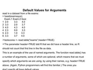
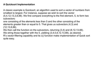
This document discusses basic loops and functions in R programming. It covers control statements like loops and if/else, arithmetic and boolean operators, default argument values, and returning values from functions. It also describes R programming structures, recursion, and provides an example of implementing quicksort recursively and constructing a binary search tree. The key topics are loops, control flow, functions, recursion, and examples of sorting and binary trees.

1. STATISTICS with R PROGRAMMING
Basic loops and functions
in r

2. R Programming Structures
Control Statements
Loops, - Looping Over Nonvector Sets,- If-Else
Arithmetic and Boolean Operators and values
Default Values for Argument, Return Values
Deciding Whether to explicitly call return- Returning Complex
Objects
Functions are Objective
No Pointers in R
Recursion
A Quick sort Implementation-Extended
Extended Example: A
Binary Search Tree.

3. R Programming Structures
R is a full programming language, similar to scripting languages such as Perl
and Python. One can define functions, use constructs such as loops and
conditionals, etc.
R is also block-structured, in a manner similar to those of the above
languages, as well as C. Blocks are delineated by braces, though they are
optional if the block consists of just a single statement.

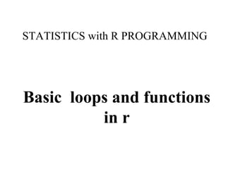
4. Control Statements
Loops
Basic Structure
In our function oddcount() the line
for (n in x) {
will be instantly recognized by Python programmers. It of course means that
there will be one iteration of
the loop for each component of the vector x, with n taking on the values of those
components.
In otherwords, in the first iteration, n = x[1], in the second iteration n = x[2], etc.
For example:
> x <- c(5,12,13)
> for (n in x) print(nˆ2)
[1] 25
[1] 144
[1] 169
C-style looping with while and repeat are also available, complete with break:

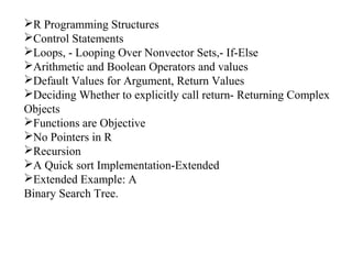
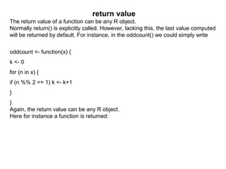
5. > i <- 1
> while(1) {
+ i <- i+4
+ if (i > 10) break
+ }
> i
[1] 13
Of course, break can be used with for too.
Another useful statement is next, which instructs the interpreter to go to the next
iteration of the loop.
Usage of this construct often allows one to avoid using complexly nested if-then-
else statements, which make the
code confusing.

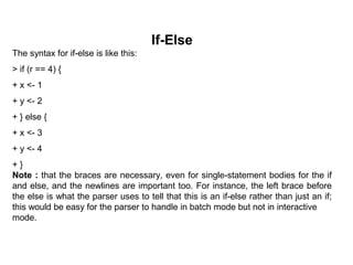
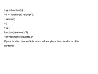
6. Looping Over Nonvector Sets
The for construct works on any vector, regardless of mode. One can loop over a
vector of file names, for
instance. Say we have files x and y with contents
1
2
3
4
5
6
and
5
12
13
Then this loop prints each of them:
> for (fn in c("x","y")) print(scan(fn))
Read 6 items
[1] 1 2 3 4 5 6
Read 3 items
[1] 5 12 13
R does not directly support iteration over nonvector sets, but there are indirect
yet easy ways to accomplish
it. One way would be to use lapply()

7. get(), as in the
following example. Here we have two matrices, u and v, containing statistical data,
and we wish to apply R
linear regression function lm() to each of them:
> u
[,1] [,2]
[1,] 1 1
[2,] 2 2
[3,] 3 4
> v
[,1] [,2]
[1,] 8 15
[2,] 12 10
[3,] 20 2
> for (m in c("u","v")) {
+ z <- get(m)
+ print(lm(z[,2] ˜ z[,1]))

8. Call:
lm(formula = z[, 2] ˜ z[, 1])
Coefficients:
(Intercept) z[, 1]
-0.6667 1.5000
Call:
lm(formula = z[, 2] ˜ z[, 1])
Coefficients:
(Intercept) z[, 1]
23.286 -1.071
The reader is welcome to make his/her own refinements here.

9. If-Else
The syntax for if-else is like this:
> if (r == 4) {
+ x <- 1
+ y <- 2
+ } else {
+ x <- 3
+ y <- 4
+ }
Note : that the braces are necessary, even for single-statement bodies for the if
and else, and the newlines are important too. For instance, the left brace before
the else is what the parser uses to tell that this is an if-else rather than just an if;
this would be easy for the parser to handle in batch mode but not in interactive
mode.

10. Arithmetic and Boolean Operators and Values
x + y addition
x - y subtraction
x * y multiplication
x / y division
x ˆ y exponentiation
x %% y modular arithmetic
x %/% y integer division
x == y test for equality
x <= y test for less-than-or-equal
x >= y test for greater-than-or-equal
x && y boolean and for scalars
x || y boolean or for scalars
x & y boolean and for vectors (vector x,y,result)
x | y boolean or for vectors (vector x,y,result)
!x boolean negation
The boolean values are TRUE and FALSE. They can be abbreviated to T and F, but
must be capitalized.

11. These values change to 1 and 0 in arithmetic expressions, e.g.
> 1 < 2
[1] TRUE
> (1 < 2) * (3 < 4)
[1] 1
> (1 < 2) * (3 < 4) * (5 < 1)
[1] 0
> (1 < 2) == TRUE
[1] TRUE
> (1 < 2) == 1
[1] TRUE

12. Default Values for Arguments
read in a dataset from a file exams:
> head(examsquiz)
Exam.1 Exam.2 Quiz
1 2.0 3.3 4.0
2 3.3 2.0 3.7
3 4.0 4.3 4.0
4 2.3 0.0 3.3
5 2.3 1.0 3.3
6 3.3 3.7 4.0
testscores <- read.table("exams",header=TRUE)
The parameter header=TRUE told R that we did have a header line, so R
should not count that first line in the file as data.
This is an example of the use of named arguments. The function read.table() has
a number of arguments, some of which are optional, which means that we must
specify which arguments we are using, by using their names, e.g. header=TRUE
above. (Again, Python programmers will find this familiar.) The ones you

13. return value
The return value of a function can be any R object.
Normally return() is explicitly called. However, lacking this, the last value computed
will be returned by default. For instance, in the oddcount() we could simply write
oddcount <- function(x) {
k <- 0
for (n in x) {
if (n %% 2 == 1) k <- k+1
}
}
Again, the return value can be any R object.
Here for instance a function is returned:

14. > g <- function() {
+ t <- function(x) return(xˆ2)
+ return(t)
+ }
> g()
function(x) return(xˆ2)
<environment: 0x8aafde8>
If your function has multiple return values, place them in a list or other
container

15. Deciding Whether to Explicitly Call return()
The prevailing R idiom is to avoid explicit calls to return(). One of the reasons cited for
this approach is that calling that function lengthens execution time. However, unless the
function is very short, the time saved is negligible, so this might not be the most
compelling reason to refrain from using return(). But it usually isn’t needed nonetheless.
Consider our second example from the preceding section:
oddcount <- function(x) {
k <- 0
for (n in x) {
if (n %% 2 == 1) k <- k+1
}
k
}

16. Returning Complex Objects
Since the return value can be any R object, you can return complex objects. Here is
an example of a function being returned:
> g
function() {
t <- function(x) return(x^2)
return(t)
}
> g()
function(x) return(x^2)
<environment: 0x8aafbc0>
If your function has multiple return values, place them in a list or other container.

17. Functions Are Objects
R functions are first-class objects (of the class "function", of course), meaning that
they can be used for the most part just like other objects. This is seen in the
syntax of function creation:
> g <- function(x) {
+ return(x+1)
+ }
Here, function() is a built-in R function whose job is to create functions! On the
right-hand side, there are really two arguments to function(): The first is the formal
argument list for the function we’re creating—here, just x—and the second is the
body of that function—here, just the single statement return(x+1). That second
argument must be of class "expression". So, the point is that the right-hand side
creates a function object, which is then assigned to g.
By the way, even the "{" is a function, as you can verify by typing this:
> ?"{"
Its job is the make a single unit of what could be several statements. These two
arguments to function() can later be accessed via the R functions
formals() and body(), as follows:
> formals(g)
$x
> body(g)
{
return(x + 1)

18. No Pointers in R
R does not have variables corresponding to pointers or references like those of,
say, the C language. This can make programming more difficult in some cases.
(As of this writing, the current version of R has an experimental feature called
reference classes, which may reduce the difficulty.)
For example, you cannot write a function that directly changes its arguments.
>>> x = [13,5,12]
>>> x.sort()
>>> x
[5, 12, 13]
Here, the value of x, the argument to sort(), changed. By contrast, here’s
how it works in R:
> x <- c(13,5,12)
> sort(x)
[1] 5 12 13
> x
[1] 13 5 12

19. Recursion
Recursion can be a powerful tool. Well then, what is it? A recursive function calls
itself. If you have not encountered this concept before, it may sound odd, but the
idea is actually simple. In rough terms, the idea is this:
To solve a problem of type X by writing a recursive function f():
1. Break the original problem of type X into one or more smaller
problems of type X.
2. Within f(), call f() on each of the smaller problems.
3. Within f(), piece together the results of (b) to solve the original
problem.

20. A Quicksort Implementation
A classic example is Quicksort, an algorithm used to sort a vector of numbers
from smallest to largest. For instance, suppose we wish to sort the vector
(5,4,12,13,3,8,88). We first compare everything to the first element, 5, to form two
subvectors:
one consisting of the elements less than 5 and the other consisting of the
elements greater than or equal to 5. That gives us subvectors (4,3) and
(12,13,8,88).
We then call the function on the subvectors, returning (3,4) and (8,12,13,88).
We string those together with the 5, yielding (3,4,5,8,12,13,88), as desired.
R’s vector-filtering capability and its c() function make implementation of Quick
sort quite easy.
NOTE This example is for the purpose of demonstrating recursion. R’s own sort
function,
sort(), is much faster, as it is written in C.

21. qs <- function(x) {
if (length(x) <= 1) return(x)
pivot <- x[1]
therest <- x[-1]
sv1 <- therest[therest < pivot]
sv2 <- therest[therest >= pivot]
sv1 <- qs(sv1)
sv2 <- qs(sv2)
return(c(sv1,pivot,sv2))
}
if (length(x) <= 1) return(x)

22. Recursion has two potential drawbacks:
• It’s fairly abstract. I knew that the graduate student, as a fine mathematician,
would take to recursion like a fish to water, because recursion is really just the
inverse of proof by mathematical induction. But many programmers find it
tough.
• Recursion is very lavish in its use of memory, which may be an issue in R if
applied to large problems

23. Extended Example: A Binary Search Tree
stored 8 in the root—that is, the head—of the tree. Its two child nodes contain 5
and 20, and the former itself has two child nodes, which store 2 and 6.
> x <- newtree(8,3)
> x
$mat
[,1] [,2] [,3]
[1,] NA NA 8
[2,] NA NA NA
[3,] NA NA NA
$nxt
[1] 2
$inc
[1] 3
> x <- ins(1,x,5)
> x

24. $mat
[,1] [,2] [,3]
[1,] 2 NA 8
[2,] NA NA 5
[3,] NA NA NA
$nxt
[1] 3
$inc
[1] 3
> x <- ins(1,x,6)
> x
$mat
[,1] [,2] [,3]
[1,] 2 NA 8
[2,] NA 3 5
[3,] NA NA 6
$nxt
[1] 4
$inc
[1] 3
> x <- ins(1,x,2)
> x

25. $mat
[,1] [,2] [,3]
[1,] 2 NA 8
[2,] 4 3 5
[3,] NA NA 6
[4,] NA NA 2
[5,] NA NA NA
[6,] NA NA NA
$nxt
[1] 5
$inc
[1] 3
> x <- ins(1,x,20)
> x
$mat
[,1] [,2] [,3]
[1,] 2 5 8
[2,] 4 3 5
[3,] NA NA 6
[4,] NA NA 2
[5,] NA NA 20
[6,] NA NA NA

26. $nxt
[1] 6
$inc
[1] 3
What happened here? First, the command containing our call newtree(8,3) creates
a new tree, assigned to x, storing the number 8. The argument 3 specifies that we
allocate storage room three rows at a time.
The result is that the matrix component of the list x is now as follows:
[,1] [,2] [,3]
[1,] NA NA 8
[2,] NA NA NA
[3,] NA NA NA

27. A Quicksort Implementation
A classic example is Quicksort, an algorithm used to sort a vector of numbers from
smallest to largest. For instance, suppose we wish to sort the vector
(5,4,12,13,3,8,88). We first compare everything to the first element, 5, to form two
subvectors:
one consisting of the elements less than 5 and the other consisting of the
elements greater than or equal to 5. That gives us subvectors (4,3) and
(12,13,8,88).
We then call the function on the subvectors, returning (3,4) and (8,12,13,88).
We string those together with the 5, yielding (3,4,5,8,12,13,88), as desired.
R’s vector-filtering capability and its c() function make implementation of Quick sort
quite easy.

28. NOTE This example is for the purpose of demonstrating recursion. R’s own sort
function,
sort(), is much faster, as it is written in C.
qs <- function(x) {
if (length(x) <= 1) return(x)
pivot <- x[1]
therest <- x[-1]
sv1 <- therest[therest < pivot]
sv2 <- therest[therest >= pivot]
sv1 <- qs(sv1)
sv2 <- qs(sv2)
return(c(sv1,pivot,sv2))
}
if (length(x) <= 1) return(x)
Without this, the function would keep calling itself repeatedly on empty vectors,
executing forever.

29. Thank U