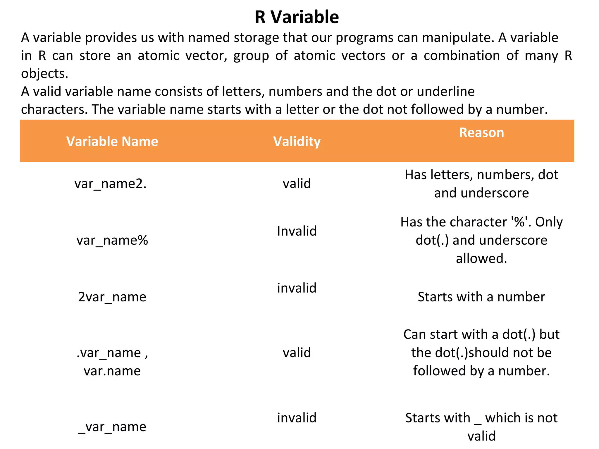
STATISTICS with R PROGRAMMING
Introduction to r language
Introduction
How to run R
R Sessions and Functions
Basic Math
Variables
Data Types
Vectors
Conclusion
Advanced Data Structures
Data Frames
Lists
Matrices
Arrays
Classes
R is an open source programming language and software environment for statistical
computing and graphics that is supported by the R Foundation for Statistical Computing.
The R language is widely used among statisticians and data miners for developing
statistical software and data analysis. Polls, surveys of data miners, and studies of
scholarly literature databases show that R's popularity has increased substantially in recent
years.
R is a GNU package. The source code for the R software environment is written primarily
in C, Fortran, and R. R is freely available under the GNU General Public License, and pre-
compiled binary versions are provided for various operating systems. While R has a
command line interface, there are several graphical front-ends available.
R is an implementation of the S programming language combined with lexical scoping
semantics inspired by Scheme. S was created by John Chambers while at Bell Labs. There
are some important differences, but much of the code written for S runs unaltered.
R was created by Ross Ihaka and Robert Gentleman[
at the University of Auckland, New
Zealand, and is currently developed by the R Development Core Team, of which Chambers
is a member. R is named partly after the first names of the first two R authors and partly
as a play on the name of S. The project was conceived in 1992, with an initial version
released in 1995 and a stable beta version in 2000.
Statistical features
R and its libraries implement a wide variety of statistical and graphical techniques,
including linear and nonlinear modeling, classical statistical tests, time-series analysis,
classification, clustering, and others.
Another strength of R is static graphics, which can produce publication-quality graphs,
including mathematical symbols. Dynamic and interactive graphics are available
through additional packages.
Programming features
R is an interpreted language, users typically access it through a command-line
interpreter.
"C:Program FilesRR-3.4.0bini386Rgui.exe“
Open R (Double Click on Desktop Icon or Open Program from START)
Click on File → Open Script
Select the Program you want to run, it will appear in a R Editor Window
Working with R session
Once we are inside the R session, we can directly execute R language commands by
typing them line by line. Pressing the enter key terminates typing of command and brings
the > prompt again. In the example session below, we declare 2 variables 'a' and 'b' to
have values 5 and 6 respectively, and assign their sum to another variable called 'c':
> a = 5
> b = 6
> c = a + b
> c
The value of the variable 'c' is printed as,
[1] 11
A function is a set of statements organized together to perform a specific task. R has a
large number of in-built functions and the user can create their own functions.
In R, a function is an object so the R interpreter is able to pass control to the function,
along with arguments that may be necessary for the function to accomplish the
actions.
The function in turn performs its task and returns control to the interpreter as well as
any
result which may be stored in other objects.
Function Definition
An R function is created by using the keyword function. The basic syntax of an R
function
definition is as follows:
function_name <- function(arg_1, arg_2, ...) {
Function body
}
Function Components
The different parts of a function are:
Function Name: This is the actual name of the function. It is stored in R
environment as an object with this name.
Arguments: An argument is a placeholder. When a function is invoked, you pass
a value to the argument. Arguments are optional; that is, a function may contain
no arguments. Also arguments can have default values.
Function Body: The function body contains a collection of statements that defines
what the function does.
Return Value: The return value of a function is the last expression in the function
body to be evaluated.
R has many in-built functions which can be directly called in the program without
defining
them first. We can also create and use our own functions referred as user
defined functions.
Built-in Function
Simple examples of in-built functions are seq(), mean(), max(), sum(x)and paste(...) etc.
They are directly called by user written programs. You can refer most widely used R
functions.
# Create a sequence of numbers from 32 to 44.
print(seq(32,44))
# Find mean of numbers from 25 to 82.
print(mean(25:82))
# Find sum of numbers frm 41 to 68.
print(sum(41:68))
When we execute the above code, it produces the following result:
[1] 32 33 34 35 36 37 38 39 40 41 42 43 44
[1] 53.5
[1] 1526
User-defined Function
We can create user-defined functions in R. They are specific to what a user wants and
once created they can be used like the built-in functions. Below is an example of how a
function is created and used.
# Create a function to print squares of numbers in sequence.
new.function <- function(a) {
for(i in 1:a) {
b <- i^2
print(b)
}
}
Calling a Function
# Create a function to print squares of numbers in sequence.
new.function <- function(a) {
for(i in 1:a) {
b <- i^2
print(b)
}
}
# Call the function new.function supplying 6 as an argument.
Calling a Function without an Argument
# Create a function without an argument.
new.function <- function() {
for(i in 1:5) {
print(i^2)
}
}
# Call the function without supplying an argument.
new.function()
When we execute the above code, it produces the following result:
[1] 1
[1] 4
[1] 9
[1] 16
[1] 25
Calling a Function with Argument Values (by position and by name)
The arguments to a function call can be supplied in the same sequence as defined in the
function or they can be supplied in a different sequence but assigned to the names of the
arguments.
# Create a function with arguments.
new.function <- function(a,b,c) {
result <- a*b+c
print(result)
}
R Programming
41
# Call the function by position of arguments.
new.function(5,3,11)
# Call the function by names of the arguments.
new.function(a=11,b=5,c=3)
When we execute the above code, it produces the following result:
[1] 26
[1] 58
Calling a Function with Default Argument
We can define the value of the arguments in the function definition and call the function
without supplying any argument to get the default result. But we can also call such
functions by supplying new values of the argument and get non default result.
# Create a function with arguments.
new.function <- function(a = 3,b =6) {
result <- a*b
print(result)
}
# Call the function without giving any argument.
new.function()
# Call the function with giving new values of the argument.
new.function(9,5)
When we execute the above code, it produces the following result:
[1] 18
[1] 45
R can perform the usual mathematical operations
Arithmetic
+ – addition
– – subtraction
* – multiplication
/ – division
Trigonometry
sin – sine
cos – cosine
tan – tangent
asin – sine inverse
acos – cosine inverse
atan – tangent inverse
Linear Algebra
+ – element-wise addition
– – element-wise subtraction
* – element-wise multiplication
/ – element-wise division
%*% – matrix multiplication
t – transpose
eigen – eigenvalues and eigenvectors
solve – inverse of matrix
ginv – generalized inverse, requires
MASS package
rbind – combines vectors of observations
horizontally into matrix class
cbind – combines vectors of observations
vertically into matrix class
R Variable
A variable provides us with named storage that our programs can manipulate. A variable
in R can store an atomic vector, group of atomic vectors or a combination of many R
objects.
A valid variable name consists of letters, numbers and the dot or underline
characters. The variable name starts with a letter or the dot not followed by a number.
Variable Name Validity
Reason
var_name2. valid
Has letters, numbers, dot
and underscore
var_name%
Invalid
Has the character '%'. Only
dot(.) and underscore
allowed.
2var_name
invalid
Starts with a number
.var_name ,
var.name
valid
Can start with a dot(.) but
the dot(.)should not be
followed by a number.
_var_name
invalid Starts with _ which is not
valid
R has 6 (although we will not discuss the raw class for this workshop) atomic vector
types.
character
numeric (real or decimal)
integer
logical
complex
By atomic, we mean the vector only holds data of a single type.
character: "a", "swc"
numeric: 2, 15.5
integer: 2L (the L tells R to store this as an integer)
logical: TRUE, FALSE
complex: 1+4i (complex numbers with real and imaginary parts)
R provides many functions to examine features of vectors and other objects, for
example
class() - what kind of object is it (high-level)?
typeof() - what is the object’s data type (low-level)?
length() - how long is it? What about two dimensional objects?
attributes() - does it have any metadata?
Vectors
When you want to create vector with more than one element, you should use c()
function
which means to combine the elements into a vector.
# Create a vector.
apple <- c('red','green',"yellow")
print(apple)
# Get the class of the vector.
print(class(apple))
When we execute the above code, it produces the following result:
[1] "red" "green" "yellow"
[1] "character"
data frame
A data frame is a table or a two-dimensional array-like structure in which each column
contains values of one variable and each row contains one set of values from each
column.
Following are the characteristics of a data frame.
The column names should be non-empty.
The row names should be unique.
The data stored in a data frame can be of numeric, factor or character type.
Each column should contain same number of data items.
Create Data Frame
# Create the
data frame. emp.data <- data.frame( emp_id = c (1:5),
emp_name = c("Rick","Dan","Michelle","Ryan","Gary"),
salary = c(623.3,515.2,611.0,729.0,843.25),
start_date = as.Date(c("2012-01-01", "2013-09-23", "2014-11-15", "2014-05-11", "2015-
03-27")),
stringsAsFactors = FALSE )
# Print the data frame. print(emp.data)
Lists
Lists are the R objects which contain elements of different types
like − numbers, strings, vectors and another list inside it. A list can
also contain a matrix or a function as its elements. List is created
using list() function.
Creating a List
Following is an example to create a list containing strings, numbers,
vectors and a logical values
# Create a list containing strings, numbers, vectors and a logical
values.
list_data <- list("Red", "Green", c(21,32,11), TRUE, 51.23, 119.1)
print(list_data)
Matrices
Matrices are the R objects in which the elements are arranged in a two-
dimensional rectangular layout. They contain elements of the same atomic
types. Though we can create a matrix containing only characters or only logical
values, they are not of much use. We use matrices containing numeric
elements to be used in mathematical calculations.
A Matrix is created using the matrix() function.
Syntax
The basic syntax for creating a matrix in R is −
matrix(data, nrow, ncol, byrow, dimnames) Following is the description of the
parameters used −
data is the input vector which becomes the data elements of the matrix.
nrow is the number of rows to be created.
ncol is the number of columns to be created.
byrow is a logical clue. If TRUE then the input vector elements are arranged by
row.
dimname is the names assigned to the rows and columns.
Example
Create a matrix taking a vector of numbers as input
# Elements are arranged sequentially by row.
M <- matrix(c(3:14), nrow = 4, byrow = TRUE)
print(M)
# Elements are arranged sequentially by column.
N <- matrix(c(3:14), nrow = 4, byrow = FALSE)
print(N)
# Define the column and row names.
rownames = c("row1", "row2", "row3", "row4") colnames = c("col1", "col2", "col3")
P <- matrix(c(3:14), nrow = 4, byrow = TRUE, dimnames = list(rownames, colnames))
print(P)
Arrays
Arrays are the R data objects which can store data in more than
two dimensions. For example − If we create an array of dimension
(2, 3, 4) then it creates 4 rectangular matrices each with 2 rows
and 3 columns. Arrays can store only data type.
An array is created using the array() function. It takes vectors as
input and uses the values in the dim parameter to create an array.
Example
The following example creates an array of two 3x3 matrices each
with 3 rows and 3 columns.
# Create two vectors of different lengths.
vector1 <- c(5,9,3)
vector2 <- c(10,11,12,13,14,15)
# Take these vectors as input to the
array. result <- array(c(vector1,vector2),dim = c(3,3,2))
print(result)
Classes
R is an object-oriented language. Objects are instances of classes. Classes are a bit more
abstract than the data types you’ve met so far. Here, we’ll look briefly at the concept using
R’s S3 classes. (The name stems from their use in the old S language, version 3, which
was the inspiration for R.) Most of R is based on these classes, and they are exceedingly
simple. Their instances are simply R lists but with an extra attribute: the class name.
For example, we noted earlier that the (nongraphical) output of the hist() histogram
function is a list with various components, such as break and count components. There
was also an attribute, which specified the class of the list, namely histogram.
> print(hn)
$breaks
[1] 400 500 600 700 800 900 1000 1100 1200 1300 1400
$counts
[1] 1 0 5 20 25 19 12 11 6 1
...
...
attr(,"class")
[1] "histogram"
Thank U

Inroduction to r

  • 1.
    STATISTICS with RPROGRAMMING Introduction to r language
  • 2.
    Introduction How to runR R Sessions and Functions Basic Math Variables Data Types Vectors Conclusion Advanced Data Structures Data Frames Lists Matrices Arrays Classes
  • 3.
    R is anopen source programming language and software environment for statistical computing and graphics that is supported by the R Foundation for Statistical Computing. The R language is widely used among statisticians and data miners for developing statistical software and data analysis. Polls, surveys of data miners, and studies of scholarly literature databases show that R's popularity has increased substantially in recent years. R is a GNU package. The source code for the R software environment is written primarily in C, Fortran, and R. R is freely available under the GNU General Public License, and pre- compiled binary versions are provided for various operating systems. While R has a command line interface, there are several graphical front-ends available. R is an implementation of the S programming language combined with lexical scoping semantics inspired by Scheme. S was created by John Chambers while at Bell Labs. There are some important differences, but much of the code written for S runs unaltered. R was created by Ross Ihaka and Robert Gentleman[ at the University of Auckland, New Zealand, and is currently developed by the R Development Core Team, of which Chambers is a member. R is named partly after the first names of the first two R authors and partly as a play on the name of S. The project was conceived in 1992, with an initial version released in 1995 and a stable beta version in 2000.
  • 4.
    Statistical features R andits libraries implement a wide variety of statistical and graphical techniques, including linear and nonlinear modeling, classical statistical tests, time-series analysis, classification, clustering, and others. Another strength of R is static graphics, which can produce publication-quality graphs, including mathematical symbols. Dynamic and interactive graphics are available through additional packages. Programming features R is an interpreted language, users typically access it through a command-line interpreter.
  • 5.
    "C:Program FilesRR-3.4.0bini386Rgui.exe“ Open R(Double Click on Desktop Icon or Open Program from START) Click on File → Open Script Select the Program you want to run, it will appear in a R Editor Window
  • 6.
    Working with Rsession Once we are inside the R session, we can directly execute R language commands by typing them line by line. Pressing the enter key terminates typing of command and brings the > prompt again. In the example session below, we declare 2 variables 'a' and 'b' to have values 5 and 6 respectively, and assign their sum to another variable called 'c': > a = 5 > b = 6 > c = a + b > c The value of the variable 'c' is printed as, [1] 11
  • 7.
    A function isa set of statements organized together to perform a specific task. R has a large number of in-built functions and the user can create their own functions. In R, a function is an object so the R interpreter is able to pass control to the function, along with arguments that may be necessary for the function to accomplish the actions. The function in turn performs its task and returns control to the interpreter as well as any result which may be stored in other objects. Function Definition An R function is created by using the keyword function. The basic syntax of an R function definition is as follows: function_name <- function(arg_1, arg_2, ...) { Function body }
  • 8.
    Function Components The differentparts of a function are: Function Name: This is the actual name of the function. It is stored in R environment as an object with this name. Arguments: An argument is a placeholder. When a function is invoked, you pass a value to the argument. Arguments are optional; that is, a function may contain no arguments. Also arguments can have default values. Function Body: The function body contains a collection of statements that defines what the function does. Return Value: The return value of a function is the last expression in the function body to be evaluated. R has many in-built functions which can be directly called in the program without defining them first. We can also create and use our own functions referred as user defined functions.
  • 9.
    Built-in Function Simple examplesof in-built functions are seq(), mean(), max(), sum(x)and paste(...) etc. They are directly called by user written programs. You can refer most widely used R functions. # Create a sequence of numbers from 32 to 44. print(seq(32,44)) # Find mean of numbers from 25 to 82. print(mean(25:82)) # Find sum of numbers frm 41 to 68. print(sum(41:68)) When we execute the above code, it produces the following result: [1] 32 33 34 35 36 37 38 39 40 41 42 43 44 [1] 53.5 [1] 1526
  • 10.
    User-defined Function We cancreate user-defined functions in R. They are specific to what a user wants and once created they can be used like the built-in functions. Below is an example of how a function is created and used. # Create a function to print squares of numbers in sequence. new.function <- function(a) { for(i in 1:a) { b <- i^2 print(b) } } Calling a Function # Create a function to print squares of numbers in sequence. new.function <- function(a) { for(i in 1:a) { b <- i^2 print(b) } } # Call the function new.function supplying 6 as an argument.
  • 11.
    Calling a Functionwithout an Argument # Create a function without an argument. new.function <- function() { for(i in 1:5) { print(i^2) } } # Call the function without supplying an argument. new.function() When we execute the above code, it produces the following result: [1] 1 [1] 4 [1] 9 [1] 16 [1] 25
  • 12.
    Calling a Functionwith Argument Values (by position and by name) The arguments to a function call can be supplied in the same sequence as defined in the function or they can be supplied in a different sequence but assigned to the names of the arguments. # Create a function with arguments. new.function <- function(a,b,c) { result <- a*b+c print(result) } R Programming 41 # Call the function by position of arguments. new.function(5,3,11) # Call the function by names of the arguments. new.function(a=11,b=5,c=3) When we execute the above code, it produces the following result: [1] 26 [1] 58
  • 13.
    Calling a Functionwith Default Argument We can define the value of the arguments in the function definition and call the function without supplying any argument to get the default result. But we can also call such functions by supplying new values of the argument and get non default result. # Create a function with arguments. new.function <- function(a = 3,b =6) { result <- a*b print(result) } # Call the function without giving any argument. new.function() # Call the function with giving new values of the argument. new.function(9,5) When we execute the above code, it produces the following result: [1] 18 [1] 45
  • 14.
    R can performthe usual mathematical operations Arithmetic + – addition – – subtraction * – multiplication / – division Trigonometry sin – sine cos – cosine tan – tangent asin – sine inverse acos – cosine inverse atan – tangent inverse Linear Algebra + – element-wise addition – – element-wise subtraction * – element-wise multiplication / – element-wise division %*% – matrix multiplication t – transpose eigen – eigenvalues and eigenvectors solve – inverse of matrix ginv – generalized inverse, requires MASS package rbind – combines vectors of observations horizontally into matrix class cbind – combines vectors of observations vertically into matrix class
  • 15.
    R Variable A variableprovides us with named storage that our programs can manipulate. A variable in R can store an atomic vector, group of atomic vectors or a combination of many R objects. A valid variable name consists of letters, numbers and the dot or underline characters. The variable name starts with a letter or the dot not followed by a number. Variable Name Validity Reason var_name2. valid Has letters, numbers, dot and underscore var_name% Invalid Has the character '%'. Only dot(.) and underscore allowed. 2var_name invalid Starts with a number .var_name , var.name valid Can start with a dot(.) but the dot(.)should not be followed by a number. _var_name invalid Starts with _ which is not valid
  • 16.
    R has 6(although we will not discuss the raw class for this workshop) atomic vector types. character numeric (real or decimal) integer logical complex By atomic, we mean the vector only holds data of a single type. character: "a", "swc" numeric: 2, 15.5 integer: 2L (the L tells R to store this as an integer) logical: TRUE, FALSE complex: 1+4i (complex numbers with real and imaginary parts) R provides many functions to examine features of vectors and other objects, for example class() - what kind of object is it (high-level)? typeof() - what is the object’s data type (low-level)? length() - how long is it? What about two dimensional objects? attributes() - does it have any metadata?
  • 17.
    Vectors When you wantto create vector with more than one element, you should use c() function which means to combine the elements into a vector. # Create a vector. apple <- c('red','green',"yellow") print(apple) # Get the class of the vector. print(class(apple)) When we execute the above code, it produces the following result: [1] "red" "green" "yellow" [1] "character"
  • 18.
    data frame A dataframe is a table or a two-dimensional array-like structure in which each column contains values of one variable and each row contains one set of values from each column. Following are the characteristics of a data frame. The column names should be non-empty. The row names should be unique. The data stored in a data frame can be of numeric, factor or character type. Each column should contain same number of data items. Create Data Frame # Create the data frame. emp.data <- data.frame( emp_id = c (1:5), emp_name = c("Rick","Dan","Michelle","Ryan","Gary"), salary = c(623.3,515.2,611.0,729.0,843.25), start_date = as.Date(c("2012-01-01", "2013-09-23", "2014-11-15", "2014-05-11", "2015- 03-27")), stringsAsFactors = FALSE ) # Print the data frame. print(emp.data)
  • 19.
    Lists Lists are theR objects which contain elements of different types like − numbers, strings, vectors and another list inside it. A list can also contain a matrix or a function as its elements. List is created using list() function. Creating a List Following is an example to create a list containing strings, numbers, vectors and a logical values # Create a list containing strings, numbers, vectors and a logical values. list_data <- list("Red", "Green", c(21,32,11), TRUE, 51.23, 119.1) print(list_data)
  • 20.
    Matrices Matrices are theR objects in which the elements are arranged in a two- dimensional rectangular layout. They contain elements of the same atomic types. Though we can create a matrix containing only characters or only logical values, they are not of much use. We use matrices containing numeric elements to be used in mathematical calculations. A Matrix is created using the matrix() function. Syntax The basic syntax for creating a matrix in R is − matrix(data, nrow, ncol, byrow, dimnames) Following is the description of the parameters used − data is the input vector which becomes the data elements of the matrix. nrow is the number of rows to be created. ncol is the number of columns to be created. byrow is a logical clue. If TRUE then the input vector elements are arranged by row. dimname is the names assigned to the rows and columns.
  • 21.
    Example Create a matrixtaking a vector of numbers as input # Elements are arranged sequentially by row. M <- matrix(c(3:14), nrow = 4, byrow = TRUE) print(M) # Elements are arranged sequentially by column. N <- matrix(c(3:14), nrow = 4, byrow = FALSE) print(N) # Define the column and row names. rownames = c("row1", "row2", "row3", "row4") colnames = c("col1", "col2", "col3") P <- matrix(c(3:14), nrow = 4, byrow = TRUE, dimnames = list(rownames, colnames)) print(P)
  • 22.
    Arrays Arrays are theR data objects which can store data in more than two dimensions. For example − If we create an array of dimension (2, 3, 4) then it creates 4 rectangular matrices each with 2 rows and 3 columns. Arrays can store only data type. An array is created using the array() function. It takes vectors as input and uses the values in the dim parameter to create an array. Example The following example creates an array of two 3x3 matrices each with 3 rows and 3 columns. # Create two vectors of different lengths. vector1 <- c(5,9,3) vector2 <- c(10,11,12,13,14,15) # Take these vectors as input to the array. result <- array(c(vector1,vector2),dim = c(3,3,2)) print(result)
  • 23.
    Classes R is anobject-oriented language. Objects are instances of classes. Classes are a bit more abstract than the data types you’ve met so far. Here, we’ll look briefly at the concept using R’s S3 classes. (The name stems from their use in the old S language, version 3, which was the inspiration for R.) Most of R is based on these classes, and they are exceedingly simple. Their instances are simply R lists but with an extra attribute: the class name. For example, we noted earlier that the (nongraphical) output of the hist() histogram function is a list with various components, such as break and count components. There was also an attribute, which specified the class of the list, namely histogram. > print(hn) $breaks [1] 400 500 600 700 800 900 1000 1100 1200 1300 1400 $counts [1] 1 0 5 20 25 19 12 11 6 1 ... ... attr(,"class") [1] "histogram"
  • 24.