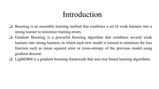
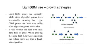
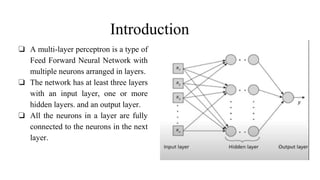
The document introduces LightGBM, a gradient boosting framework that improves training speed, accuracy, and efficiency through features like histogram-based splitting, exclusive feature bundling, and gradient-based sampling. It contrasts this with multi-layer perceptrons (MLPs), which are neural networks consisting of multiple layers with fully connected neurons for classification and regression tasks. While LightGBM handles large datasets and categorical variables effectively, it has disadvantages such as difficulty in parameter tuning and GPU configuration challenges.

1. LightGBM

2. Introduction
❏ Boosting is an ensemble learning method that combines a set of weak learners into a
strong learner to minimize training errors.
❏ Gradient Boosting is a powerful boosting algorithm that combines several weak
learners into strong learners, in which each new model is trained to minimize the loss
function such as mean squared error or cross-entropy of the previous model using
gradient descent.
❏ LightGBM is a gradient boosting framework that uses tree based learning algorithms.

3. Advantages
● Faster training speed and higher efficiency.
● Lower memory usage.
● Better accuracy.
● Support of parallel, distributed, and GPU learning.
● Capable of handling large-scale data efficiently.
● Can handle categorical variable directly without the need for one-hot encoding.

4. What Makes LightGBM faster?
1. Histogram or bin way of splitting
For e.g. BU dataset has a column CSE-Students, in which we’ve students from 6th,7th,
8th, 9th and 10th batch. Now, in other boosting methods all the batch will be tested that
won’t be minimal. So, now we can split the students into two bins, 6th-8th batch, and 9th-
10th batch. This will reduces the memory usage and speeds up the training process,.

5. What Makes LightGBM faster?(Cont.)
2. Exclusive Feature Building (EFB)
For e.g. we’re considering gender of the respondents. If the respondents is a male, it will
enter 1 in the male column, 0 in female column, or if the respondents is a female, it will
enter 1 in the female column, 0 in male column. There is no chances to enter 1 in both
column at the same time. This type of features are called exclusive feature. LightGBM
will bundle this feature, by reducing two dimension into one dimension, through creating
a new feature, such as BF, that will contain 11 for male and 10 for female.

6. What Makes LightGBM faster?(Cont.)
3. GOSS (Gradient based One Side Sampling)
● It sees a error and decide how to create this sample
● For e.g. your baseline model is M0 on 500 records, i.e. you will’ve 500 gradients or error. Let this is G1,G2,G3,…, G500.
Now LightGBM will sort it in descending order. Suppose, first gradient number 48 have have highest gradient record than 14,
and so on. So it will be now: G48, G14,..., G4.
Now certain percentage( usually 20%) from this record will be taken as one part (as top 20%) and from the remaining 80%
randomly selected certain percentage( usually 10%) will come out (as bottom subset 10%). Now these two are combined to
create new subsample.
Now If gradient is low, that means in this 80% the model performs good we don’t need to train it again and again, but if in the
20% if the model is not performing well( gradients are high , errors are high), then it should train more. As a result top will take
high priority and sampling is done only from one side(right side ,80%).

7. LightGBM tree – growth strategies
● Light GBM grows tree vertically
while other algorithm grows trees
horizontally meaning that Light
GBM grows tree leaf- wise while
other algorithm grows level- wise.
● It will choose the leaf with max
delta loss to grow. When growing
the same leaf, Leaf-wise algorithm
can reduce more loss than a level-
wise algorithm

8. Where should we use LightGBM?
❏ In our local machine, or anywhere where there is no gpu or no clustering
❏ For performing faster machine learning tasks such as classification, regression and
ranking

9. LightGBM disadvantages
● Too many parameters
● Slow to tune parameters
● GPU configuration can be tough
● No GPU support on scikit –learn API

10. Multilayer Perceptron (MLP)

11. Introduction
❏ A multi-layer perceptron is a type of
Feed Forward Neural Network with
multiple neurons arranged in layers.
❏ The network has at least three layers
with an input layer, one or more
hidden layers. and an output layer.
❏ All the neurons in a layer are fully
connected to the neurons in the next
layer.

12. Working Process
❏ The input layer is the visible layer.
❏ It just passes the input to the next
layer.
❏ The layers following the input layer
are the hidden layers.
❏ The hidden layers neither directly
receive inputs nor send outputs to
the external environment.
❏ The final layer is the output layer
which outputs a single value or a
vector of values.

13. Working Process(Cont.)
❏ The activation functions used in the
layers can be linear or non-linear
depending on the type of the
problem modelled.
❏ Typically, a sigmoid activation
function is used if the problem is a
binary classification problem and a
softmax activation function is used
in a multi-class classification
problem.

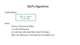
14. MLP Algorithms
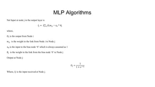
Input: Input vector (x1, x2 ......, xn)
Output: Yn
Learning rate: α
Assign random weights and biases for every connection in the network in the range [-0.5, +0.5].
Step 1: Forward Propagation
1. Calculate Input and Output in the Input Layer:
Input at Node j 'Ij' in the Input Layer is:
Where,
ϰj, is the input received at Node j
Output at Node j 'Oj' in the Input Layer is:

15. MLP Algorithms
Net Input at node j in the output layer is
𝐼𝑗 = 𝛴𝑖=1
𝑛
𝑂𝑖𝑤𝑖𝑗 + 𝑥0 * 𝜃𝑗
where,
𝑂𝑖 is the output from Node i
𝑤𝑖𝑗 is the weight in the link from Node i to Node j
𝑥0 is the input to the bias node ‘0’ which is always assumed as 1
𝜃𝑗 is the weight in the link from the bias node ‘0’ to Node j
Output at Node j:
𝑂𝑗 =
1
1 + ⅇ−𝐼𝑗
Where, 𝐼𝑗 is the input received at Node j.

16. MLP Algorithms
● Estimated error at the node in the Output Layer:
Error = 𝑂𝐷𝑒𝑠𝑖𝑟𝑒𝑑 - 𝑂𝐸𝑠𝑡𝑖𝑚𝑎𝑡𝑒𝑑
where,
𝑂𝐷𝑒𝑠𝑖𝑟𝑒𝑑 is the desired output value of the Node in the Output Layer
𝑂𝐸𝑠𝑡𝑖𝑚𝑎𝑡𝑒𝑑 is the estimated output value of the Node in the Output Layer

17. MLP Algorithms
● Step 2: Backward Propagation
1. Calculated Error at each node:
For each Unit k in the Output Layer
𝐸𝑟𝑟𝑜𝑟𝑘 = 𝑂𝑘(1-𝑂𝑘) (𝑂𝐷𝑒𝑠𝑖𝑟𝑒𝑑 -𝑂𝑘)
where,
𝑂𝑘 is the output value at Node k in the Output Layer
𝑂𝐷𝑒𝑠𝑖𝑟𝑒𝑑 is the desired output value at Node in the Output Layer
For each unit j in the Hidden Layer
𝐸𝑟𝑟𝑜𝑟
𝑗 = 𝑂𝑗(1-𝑂𝑗)𝛴𝑘𝐸𝑟𝑟𝑜𝑟𝑘𝑤𝑗𝑘
where,
𝑂𝑗 is the output value at Node j in the Hidden Layer
𝐸𝑟𝑟𝑜𝑟𝑘 is the error at Node k in the Output Layer
𝑤𝑗𝑘 is the weight in the link from Node j to Node k

18. MLP Algorithms
2. Update all weights and biases:
Update weights
where,
𝑂𝑖 is the output value at Node i
𝐸𝑟𝑟𝑜𝑟
𝑗 is the error at Node j
𝛼 is the learning rate
𝑤𝑖𝑗 is the weight in the link from Node i to Node j
Δ𝑤𝑖𝑗 is the difference in weight that has to be added to 𝑤𝑖𝑗
Δ𝑤𝑖𝑗 = 𝛼 * 𝐸𝑟𝑟𝑜𝑟𝑗 * 𝑂𝑖
𝑤𝑖𝑗 = 𝑤𝑖𝑗 + Δ𝑤𝑖𝑗

19. MLPs Algorithms
Update Biases
where,
𝐸𝑟𝑟𝑜𝑟𝑗 is the error at Node j
𝛼 is the learning rate
𝜃𝑗 is the bias value from Bias Node 0 to Node j.
Δ𝜃𝑗 is the difference in bias that has to be added to 𝜃𝑗.
Δ𝜃𝑗 = 𝛼 * 𝐸𝑟𝑟𝑜𝑟
𝑗
𝜃𝑗 =𝜃𝑗 + Δ𝜃𝑗