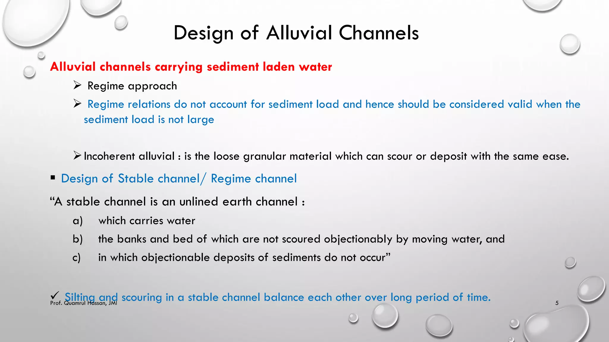
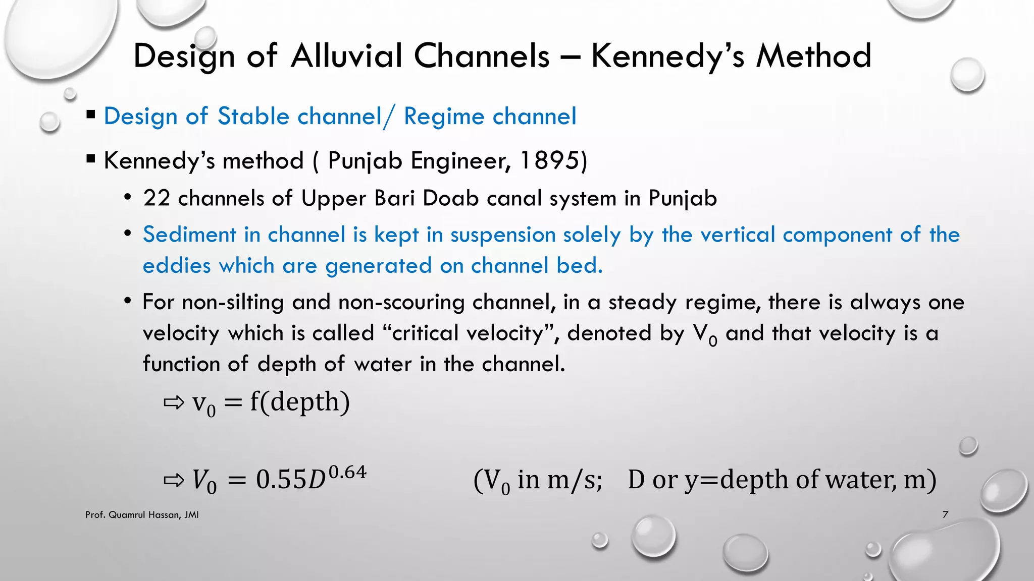
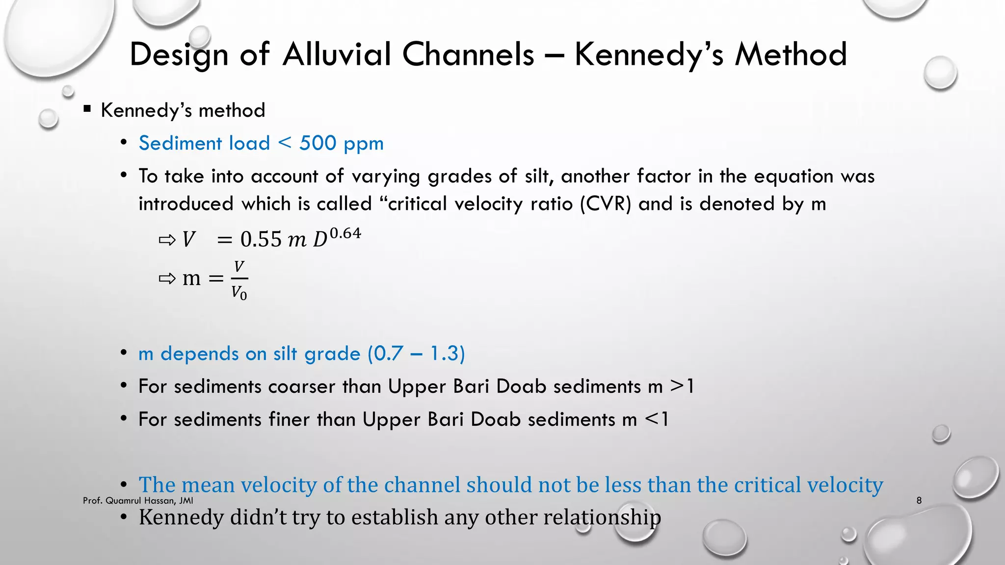
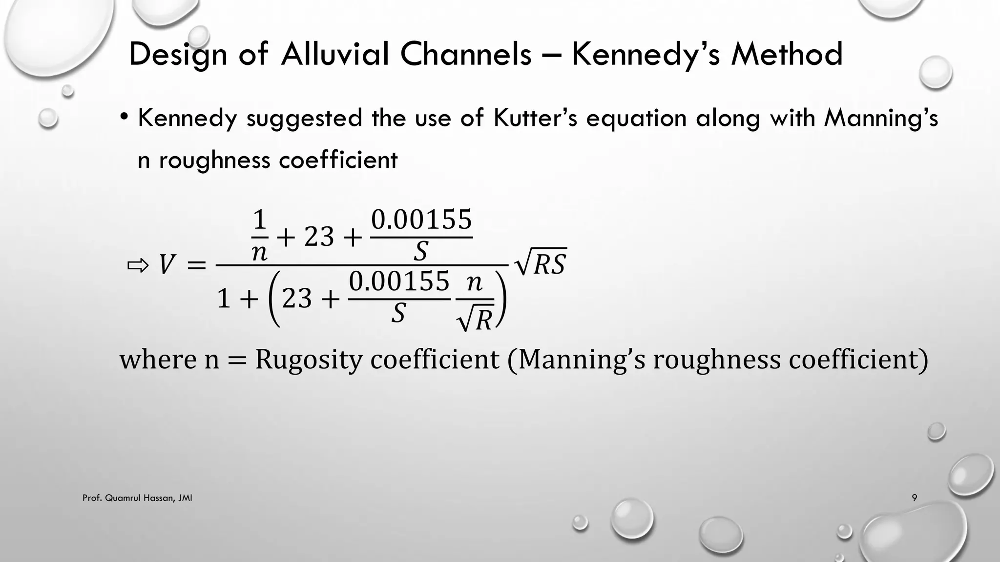
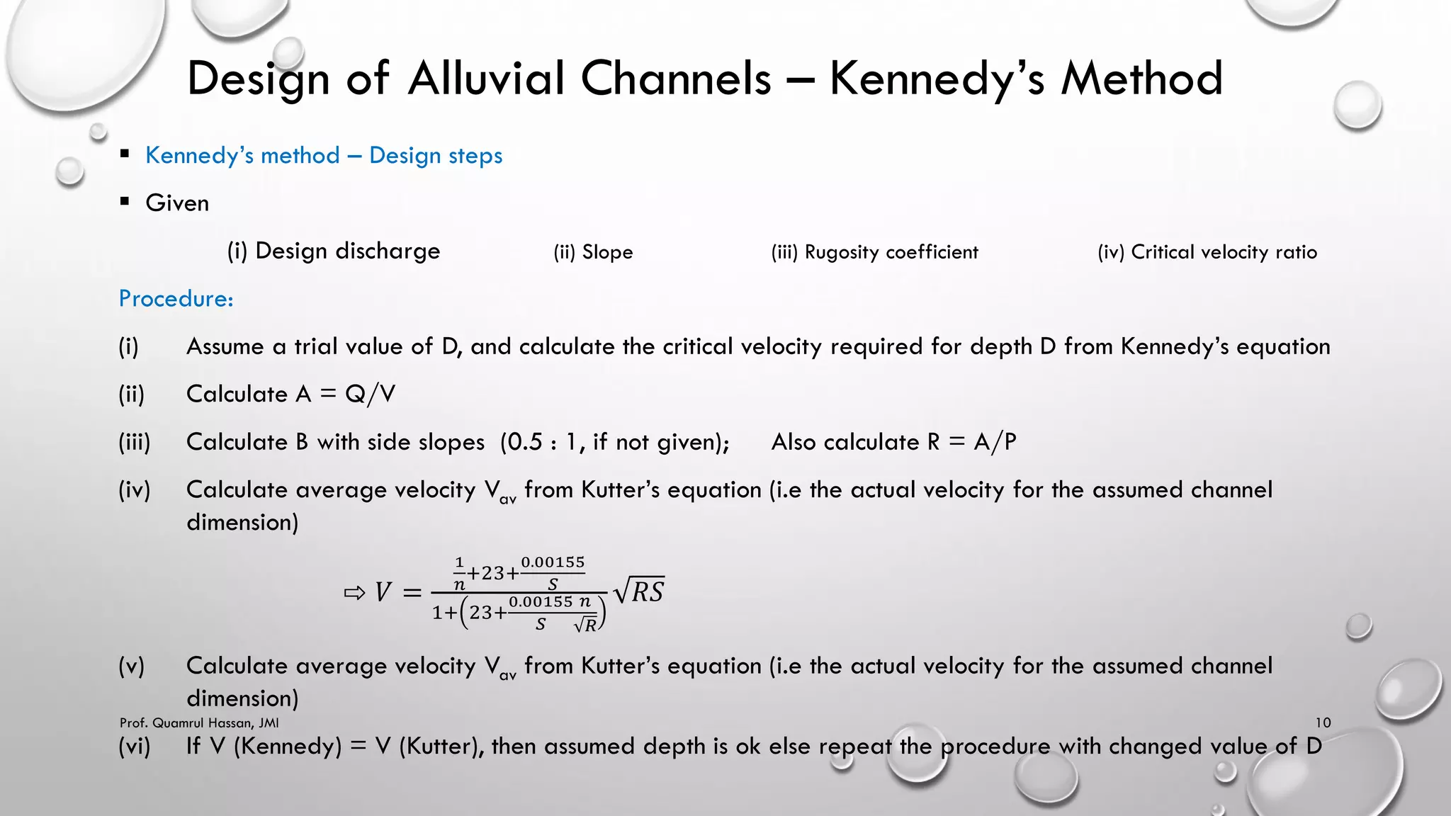
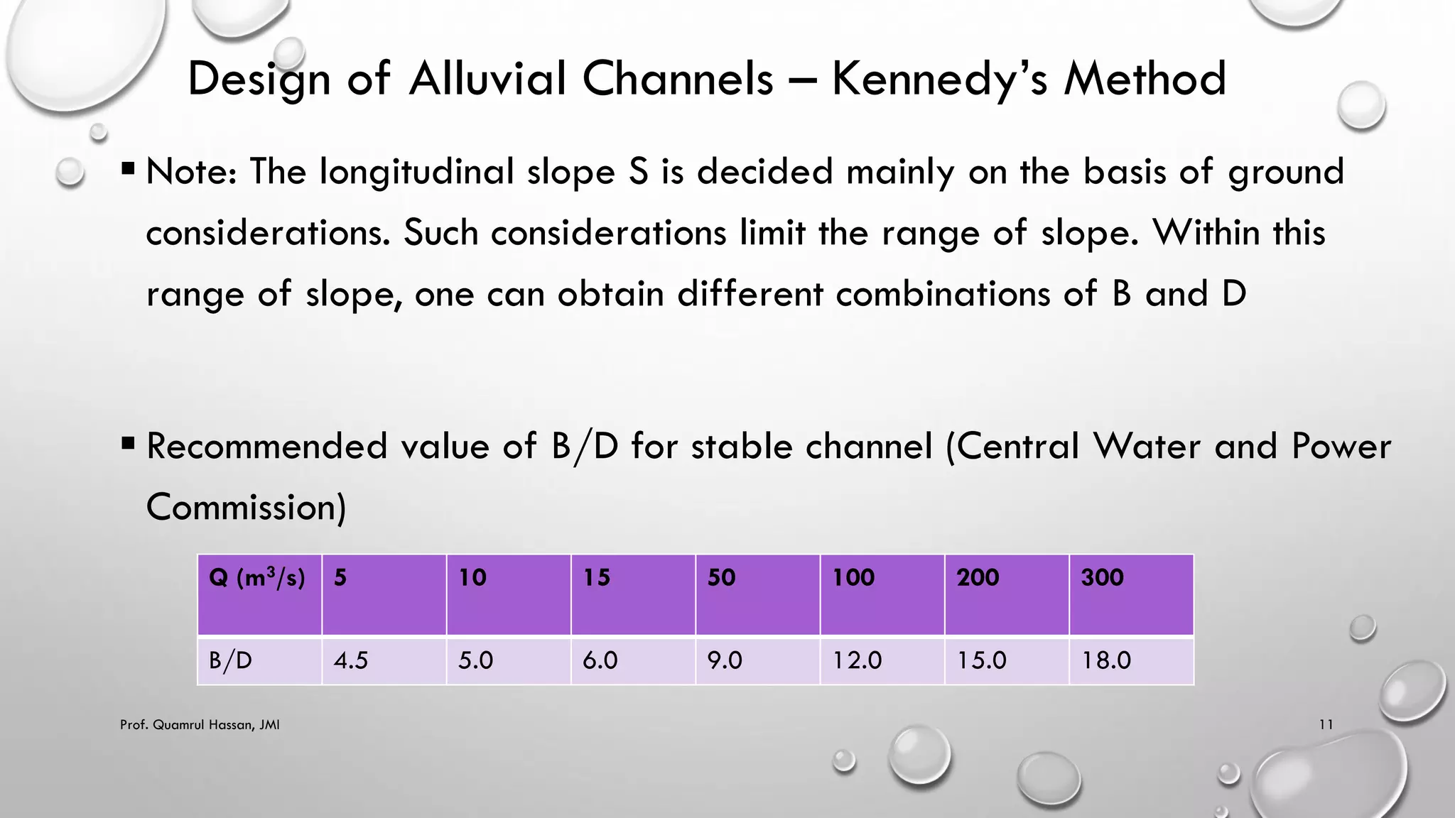
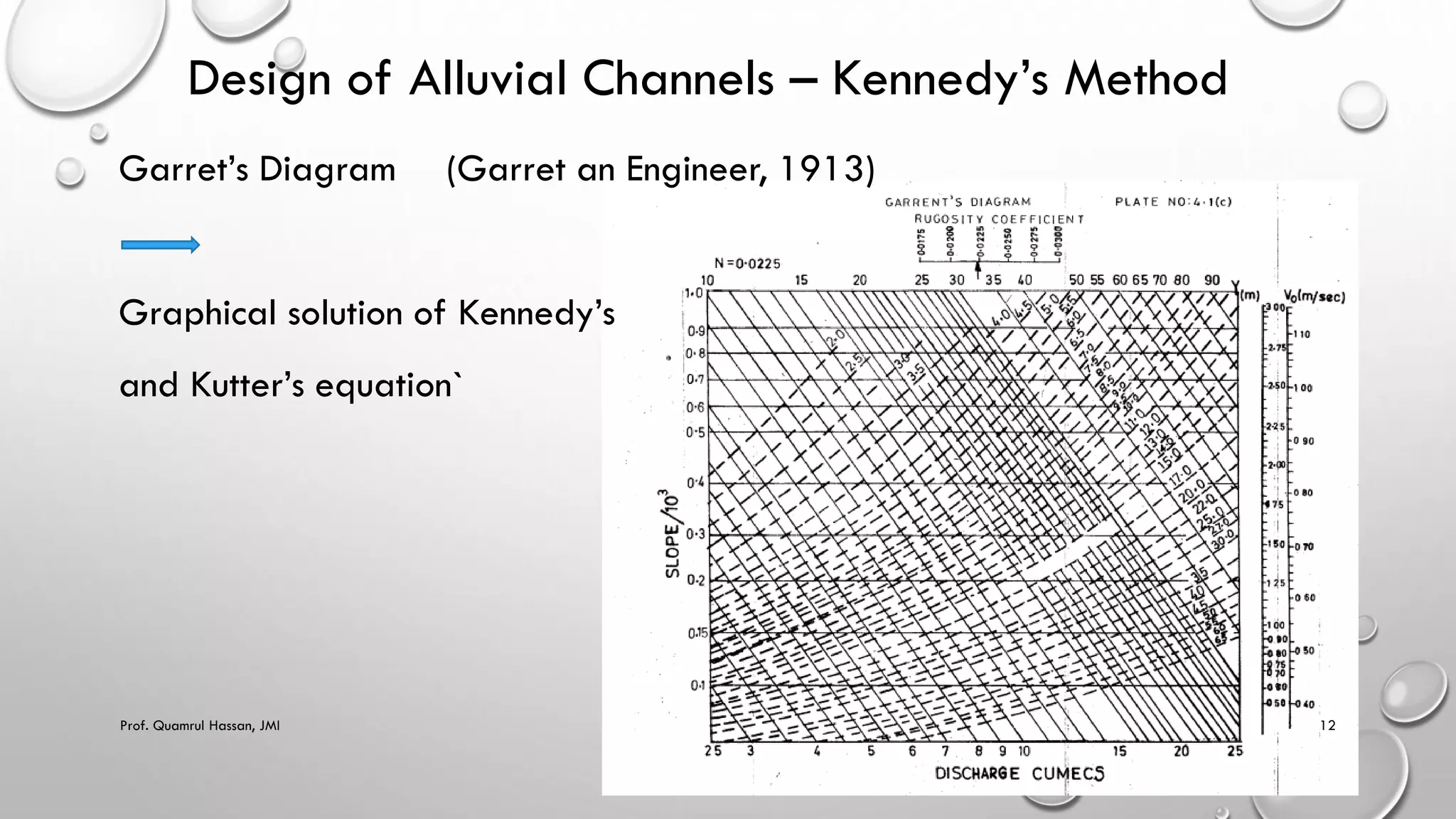
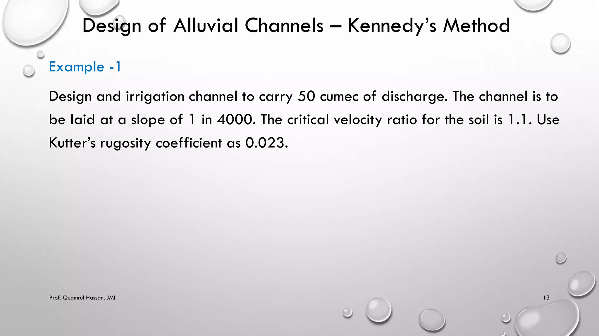
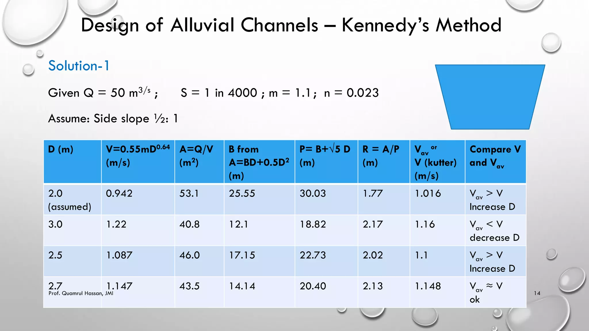
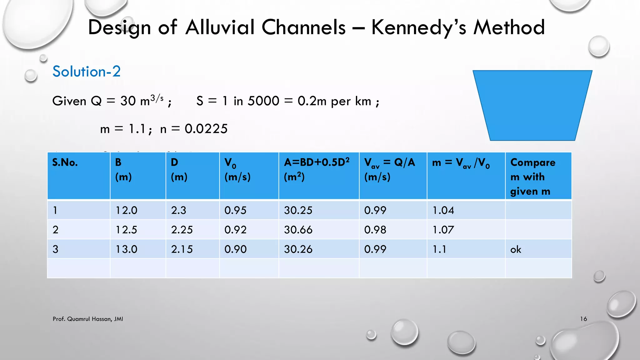
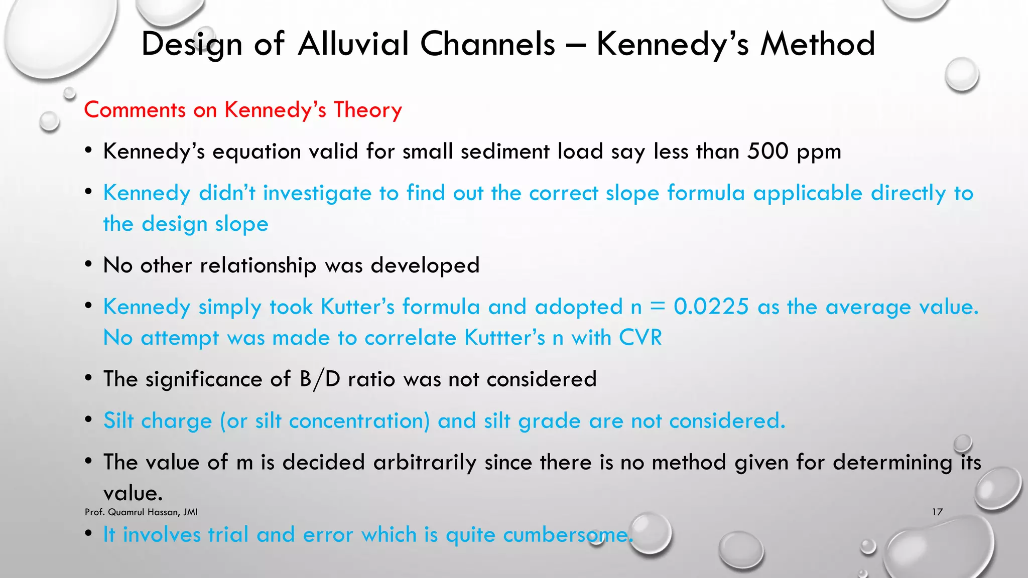
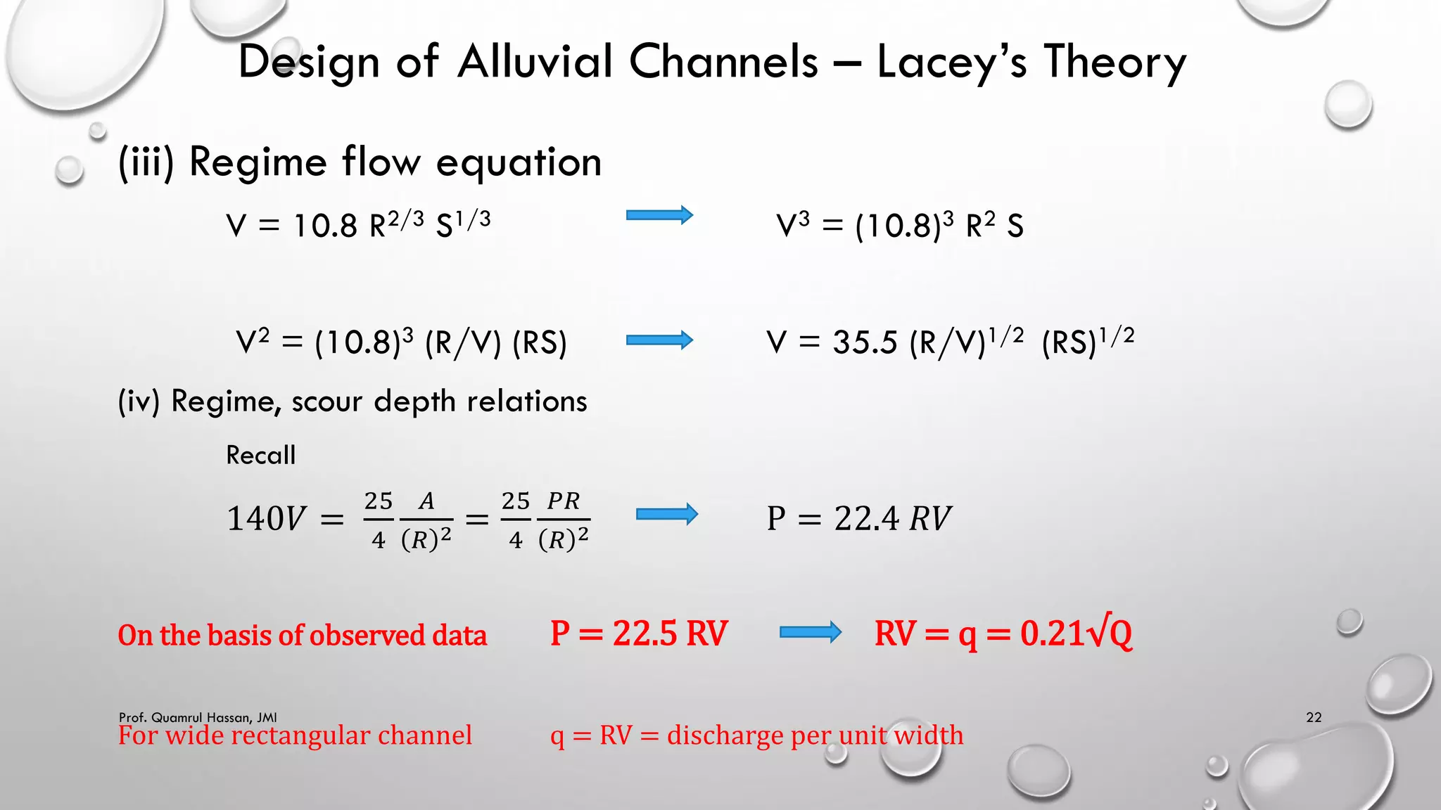
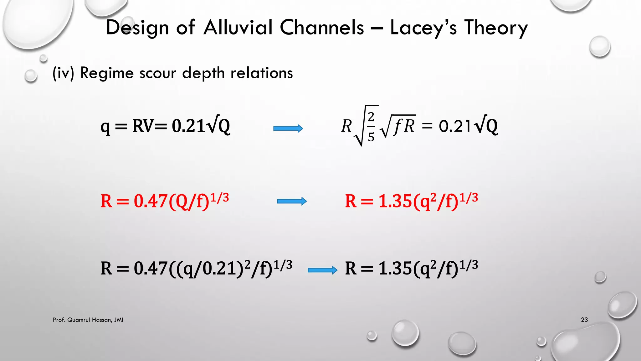
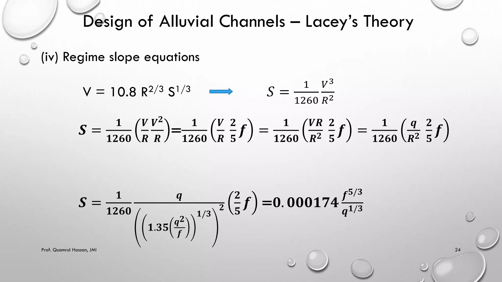
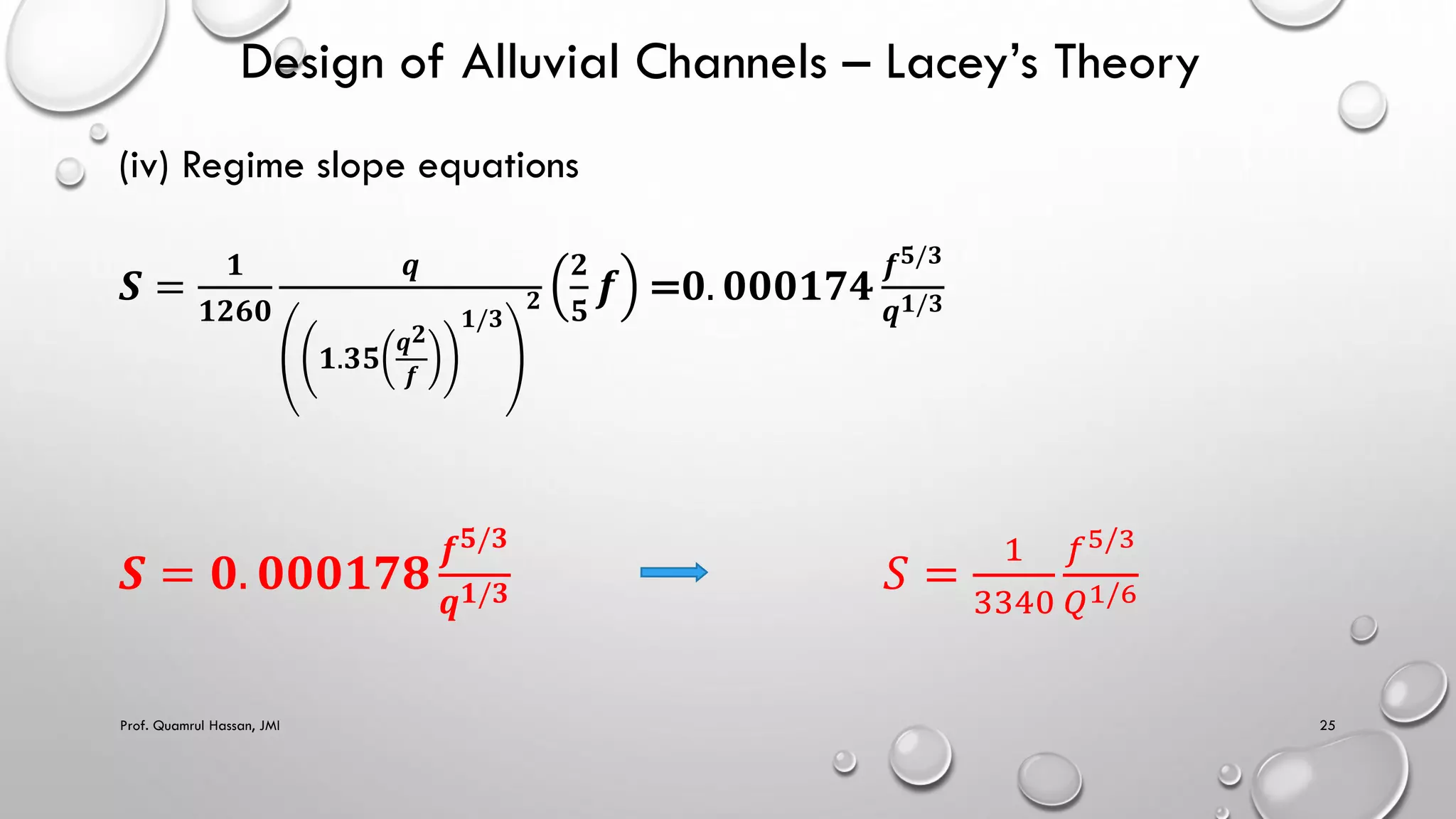
CE702 IRRIGATION ENGINEERING
Course Instructor - Prof. Quamrul Hassan
Topics to be covered
 Design of alluvial Channels
 Silt theories – problems of silting and scouring,
 Kennedy’s theory, design procedure, Use of Garret’s diagram,
drawbacks
 Lacey’s silt theory, channel design procedure, drawbacks
 Comparison between Kennedy’s and Lacey’s theory
 Lacey’s non-regime equation
 L-section of a channel, balancing depth, Cross-section of irrigation
channels.
Prof. Quamrul Hassan, JMI 3
Design of Alluvial Channels
Four types of channel
(A) Rigid boundary (i.e. non-erodible) channels carrying clean water
 Design based on limiting velocity
Q =
1
𝑛
𝐴𝑅2/3𝑆1/2
(B) Rigid boundary (i.e. non-erodible) channels carrying sediment laden water
 Minimum permissible velocity to prevent silting as well as growth of vegetation
(C) Alluvial channels carrying clean water
 Design more complex
Erodible material of the channel boundary is not scoured
Design based on the concept of tractive force (USBR method)
(D) Alluvial channels carrying sediment laden water
Prof. Quamrul Hassan, JMI 4
Design of Alluvial Channels
Alluvial channels carrying sediment laden water
 Regime approach
 Regime relations do not account for sediment load and hence should be considered valid when the
sediment load is not large
Incoherent alluvial : is the loose granular material which can scour or deposit with the same ease.
 Design of Stable channel/ Regime channel
“A stable channel is an unlined earth channel :
a) which carries water
b) the banks and bed of which are not scoured objectionably by moving water, and
c) in which objectionable deposits of sediments do not occur”
 Silting and scouring in a stable channel balance each other over long period of time.
Prof. Quamrul Hassan, JMI 5
Design of Alluvial Channels
 Design of Stable channel/ Regime channel
Design ⇨ Mean velocity, depth/hydraulic radius, width and slope of the
channel (shape and size of channel, slope)
for known value of
Q
sediment discharge QT
Sediment size d, and
the channel roughness characteristics,
Prof. Quamrul Hassan, JMI 6
Design of Alluvial Channels – Kennedy’s Method
 Design of Stable channel/ Regime channel
 Kennedy’s method ( Punjab Engineer, 1895)
• 22 channels of Upper Bari Doab canal system in Punjab
• Sediment in channel is kept in suspension solely by the vertical component of the
eddies which are generated on channel bed.
• For non-silting and non-scouring channel, in a steady regime, there is always one
velocity which is called “critical velocity”, denoted by V0 and that velocity is a
function of depth of water in the channel.
⇨ v0 = f(depth)
⇨ 𝑉0 = 0.55𝐷0.64
(V0 in m/s; D or y=depth of water, m)
Prof. Quamrul Hassan, JMI 7
Design of Alluvial Channels – Kennedy’s Method
 Kennedy’s method
• Sediment load < 500 ppm
• To take into account of varying grades of silt, another factor in the equation was
introduced which is called “critical velocity ratio (CVR) and is denoted by m
⇨ 𝑉 = 0.55 𝑚 𝐷0.64
⇨ m =
𝑉
𝑉0
• m depends on silt grade (0.7 – 1.3)
• For sediments coarser than Upper Bari Doab sediments m >1
• For sediments finer than Upper Bari Doab sediments m <1
• The mean velocity of the channel should not be less than the critical velocity
• Kennedy didn’t try to establish any other relationship
Prof. Quamrul Hassan, JMI 8
Design of Alluvial Channels – Kennedy’s Method
• Kennedy suggested the use of Kutter’s equation along with Manning’s
n roughness coefficient
⇨ 𝑉 =
1
𝑛
+ 23 +
0.00155
𝑆
1 + 23 +
0.00155
𝑆
𝑛
𝑅
𝑅𝑆
where n = Rugosity coefficient (Manning’s roughness coefficient)
Prof. Quamrul Hassan, JMI 9
Design of Alluvial Channels – Kennedy’s Method
 Kennedy’s method – Design steps
 Given
(i) Design discharge (ii) Slope (iii) Rugosity coefficient (iv) Critical velocity ratio
Procedure:
(i) Assume a trial value of D, and calculate the critical velocity required for depth D from Kennedy’s equation
(ii) Calculate A = Q/V
(iii) Calculate B with side slopes (0.5 : 1, if not given); Also calculate R = A/P
(iv) Calculate average velocity Vav from Kutter’s equation (i.e the actual velocity for the assumed channel
dimension)
⇨ 𝑉 =
1
𝑛
+23+
0.00155
𝑆
1+ 23+
0.00155
𝑆
𝑛
𝑅
𝑅𝑆
(v) Calculate average velocity Vav from Kutter’s equation (i.e the actual velocity for the assumed channel
dimension)
(vi) If V (Kennedy) = V (Kutter), then assumed depth is ok else repeat the procedure with changed value of D
Prof. Quamrul Hassan, JMI 10
Design of Alluvial Channels – Kennedy’s Method
 Note: The longitudinal slope S is decided mainly on the basis of ground
considerations. Such considerations limit the range of slope. Within this
range of slope, one can obtain different combinations of B and D
 Recommended value of B/D for stable channel (Central Water and Power
Commission)
Q (m3/s) 5 10 15 50 100 200 300
B/D 4.5 5.0 6.0 9.0 12.0 15.0 18.0
Prof. Quamrul Hassan, JMI 11
Design of Alluvial Channels – Kennedy’s Method
Garret’s Diagram (Garret an Engineer, 1913)
Graphical solution of Kennedy’s
and Kutter’s equation`
Prof. Quamrul Hassan, JMI 12
Design of Alluvial Channels – Kennedy’s Method
Example -1
Design and irrigation channel to carry 50 cumec of discharge. The channel is to
be laid at a slope of 1 in 4000. The critical velocity ratio for the soil is 1.1. Use
Kutter’s rugosity coefficient as 0.023.
Prof. Quamrul Hassan, JMI 13
Design of Alluvial Channels – Kennedy’s Method
Solution-1
Given Q = 50 m3/s ; S = 1 in 4000 ; m = 1.1; n = 0.023
Assume: Side slope ½: 1
D (m) V=0.55mD0.64
(m/s)
A=Q/V
(m2)
B from
A=BD+0.5D2
(m)
P= B+√5 D
(m)
R = A/P
(m)
Vav
or
V (kutter)
(m/s)
Compare V
and Vav
2.0
(assumed)
0.942 53.1 25.55 30.03 1.77 1.016 Vav > V
Increase D
3.0 1.22 40.8 12.1 18.82 2.17 1.16 Vav < V
decrease D
2.5 1.087 46.0 17.15 22.73 2.02 1.1 Vav > V
Increase D
2.7 1.147 43.5 14.14 20.40 2.13 1.148 Vav ≈ V
ok
Prof. Quamrul Hassan, JMI 14
Design of Alluvial Channels – Kennedy’s Method
Example -2
Design an irrigation channel to carry 30 cumec of discharge. The channel is to be laid at a
slope of 1 in 5000. The Critical velocity ratio for the soil is 1.1. Use n = 0.0225
Use Garret’s diagram also.
Prof. Quamrul Hassan, JMI 15
Design of Alluvial Channels – Kennedy’s Method
Solution-2
Given Q = 30 m3/s ; S = 1 in 5000 = 0.2m per km ;
m = 1.1; n = 0.0225
Assume: Side slope ½: 1
S.No. B
(m)
D
(m)
V0
(m/s)
A=BD+0.5D2
(m2)
Vav = Q/A
(m/s)
m = Vav /V0 Compare
m with
given m
1 12.0 2.3 0.95 30.25 0.99 1.04
2 12.5 2.25 0.92 30.66 0.98 1.07
3 13.0 2.15 0.90 30.26 0.99 1.1 ok
Prof. Quamrul Hassan, JMI 16
Design of Alluvial Channels – Kennedy’s Method
Comments on Kennedy’s Theory
• Kennedy’s equation valid for small sediment load say less than 500 ppm
• Kennedy didn’t investigate to find out the correct slope formula applicable directly to
the design slope
• No other relationship was developed
• Kennedy simply took Kutter’s formula and adopted n = 0.0225 as the average value.
No attempt was made to correlate Kuttter’s n with CVR
• The significance of B/D ratio was not considered
• Silt charge (or silt concentration) and silt grade are not considered.
• The value of m is decided arbitrarily since there is no method given for determining its
value.
• It involves trial and error which is quite cumbersome.
Prof. Quamrul Hassan, JMI 17
Design of Alluvial Channels – Lacey’s Theory
Lacey’s Theory
“According to Lacey, a channel flowing in an unlimited incoherent Alluvial of the same
grade as the material transported, if continued uninterrupted (i.e. the condition of
discharge and silt remaining constant) would attain final stability or final regime
condition”
“A channel is said to have attained a regime condition when a balance between silting
and scouring and a dynamic equilibrium in the forces generating and maintaining the
channel cross section and gradient has attained”.
“ There is only one section of a channel and only one slope at which the channel
carrying a given discharge will carry a particular grade of silt”.
Prof. Quamrul Hassan, JMI 18
Design of Alluvial Channels – Lacey’s Theory
Initial Regime » by bed slope & depth
Final regime » + bed width
• Final regime velocity = f( constant discharge, silt grade)
• Channels are usually excavated to 1:1 side slope. It is assumed that after silting
they will have side slope of approximately ½ : 1
Prof. Quamrul Hassan, JMI 19
Design of Alluvial Channels – Lacey’s Theory
Lacey originally gave two equations
𝑉 =
2
5
𝑓𝑅 (1)
Af2 = 140 V5 (2)
Where,
V = average velocity (m/s)
f = silt factor = 1.76 √d50
R = hydraulic mean radius (m)
A = area of cross section (m2)
d= mean particle size in mm
Prof. Quamrul Hassan, JMI 20
Design of Alluvial Channels – Lacey’s Theory
(i) P-Q relaltions
𝐴𝑓2
4
25
𝑓2𝑅2
=
140𝑉5
𝑉4
25
4
𝐴
𝐴
𝑃
2 = 140𝑉
25
4
𝑃2
= 140𝐴𝑉 = 140𝑄 P = 4.733√Q
On the basis of observed data P = 4.75 √Q
(ii) V-Q-f relations
V (Af2) = (140 V5) V Qf2 = 140 V6
V = (Qf2 / 140)1/6
Prof. Quamrul Hassan, JMI 21
Design of Alluvial Channels – Lacey’s Theory
(iii) Regime flow equation
V = 10.8 R2/3 S1/3 V3 = (10.8)3 R2 S
V2 = (10.8)3 (R/V) (RS) V = 35.5 (R/V)1/2 (RS)1/2
(iv) Regime, scour depth relations
Recall
140𝑉 =
25
4
𝐴
𝑅 2 =
25
4
𝑃𝑅
𝑅 2 P = 22.4 𝑅𝑉
On the basis of observed data P = 22.5 RV RV = q = 0.21√Q
For wide rectangular channel q = RV = discharge per unit width
Prof. Quamrul Hassan, JMI 22
Design of Alluvial Channels – Lacey’s Theory
(iv) Regime scour depth relations
q = RV= 0.21√Q 𝑅
2
5
𝑓𝑅 = 0.21√Q
R = 0.47(Q/f)1/3 R = 1.35(q2/f)1/3
R = 0.47((q/0.21)2/f)1/3 R = 1.35(q2/f)1/3
Prof. Quamrul Hassan, JMI 23
Design of Alluvial Channels – Lacey’s Theory
(iv) Regime slope equations
V = 10.8 R2/3 S1/3 𝑆 =
1
1260
𝑉3
𝑅2
𝑺 =
𝟏
𝟏𝟐𝟔𝟎
𝑽
𝑹
𝑽𝟐
𝑹
=
𝟏
𝟏𝟐𝟔𝟎
𝑽
𝑹
𝟐
𝟓
𝒇 =
𝟏
𝟏𝟐𝟔𝟎
𝑽𝑹
𝑹𝟐
𝟐
𝟓
𝒇 =
𝟏
𝟏𝟐𝟔𝟎
𝒒
𝑹𝟐
𝟐
𝟓
𝒇
𝑺 =
𝟏
𝟏𝟐𝟔𝟎
𝒒
𝟏.𝟑𝟓
𝒒𝟐
𝒇
𝟏/𝟑
𝟐
𝟐
𝟓
𝒇 =𝟎. 𝟎𝟎𝟎𝟏𝟕𝟒
𝒇𝟓/𝟑
𝒒𝟏/𝟑
Prof. Quamrul Hassan, JMI 24
Design of Alluvial Channels – Lacey’s Theory
(iv) Regime slope equations
𝑺 =
𝟏
𝟏𝟐𝟔𝟎
𝒒
𝟏.𝟑𝟓
𝒒𝟐
𝒇
𝟏/𝟑
𝟐
𝟐
𝟓
𝒇 =𝟎. 𝟎𝟎𝟎𝟏𝟕𝟒
𝒇𝟓/𝟑
𝒒𝟏/𝟑
𝑺 = 𝟎. 𝟎𝟎𝟎𝟏𝟕𝟖
𝒇𝟓/𝟑
𝒒𝟏/𝟑 𝑆 =
1
3340
𝑓5/3
𝑄1/6
Prof. Quamrul Hassan, JMI 25
Design of Alluvial Channels – Lacey’s Theory
Example-3
Design a regime channel for a discharge of 40 cumecs with silt factor 0.9
by Lacey’s theory
Solution:
Given: Q= 40 cumecs f = 0.9
Prof. Quamrul Hassan, JMI 26
Design of Alluvial Channels – Lacey’s Theory
Solution-3
Given: Q= 40 cumecs f = 0.9
V = (Qf2/140)1/6 = 0.783 m/s
R = (5/2) (V2/f) = 1.70 m
P = 4.75 √Q = 30.0 m
For trapezoidal channel with side slopes ½ : 1
A = BD + ½ D2 = Q/V = 40/0.783 = 51.085
P = B + √5 D = 30.0
Solving above two equations B = 26.7 m, D = 1.925 m
𝑆 =
1
3340
𝑓5/3
𝑄1/6 = 1/6670 or 15 cm per km
Prof. Quamrul Hassan, JMI 27
Comparison of Kennedy’s and Lacey’s theory
• Kennedy considered a trapezoidal channel section and therefore, neglected the eddies
generated from sides. Hence Critical velocity formula was derived only in terms of depth.
While Lacey considered that an irrigation channel achieves a cup shaped section (semi ellipse)
and that the entire wetted perimeter of the channel section contributes to the generation of
silt supporting eddies.
• Kenney stated that all the channels to be in a state of regime provided they do not silt or
scour. But Lacey differentiated between two regimes i.e. initial regime and final regime
• According to Lacey, the grain size of the material forming the channel is an important factor
and should need much more rational attention that was given to it by Kennedy.
• Kennedy used Kutter’s equation while Lacey proposed a new equation.
• Kennedy has not given any importance to bed width and depth ratio. Lacey has established
relationship for P, A and Q.
• Kennedy didn’t fix regime slope for the channel while Lacey has fixed the regime slope.
Prof. Quamrul Hassan, JMI 28
Text Books
1. Irrigation, Water Resources and Power Engineering by P.N.
Modi, Standard Book House, Delhi
2. Irrigation Engineering and Hydraulic Structures by S.K. Garg,
Khanna Publishers, Latest edition
References :-
1.Irrigation and Water Resources Engineering by G.L. Asawa,
New Age International Publishers
2.Theory and Design of Irrigation Structures by By Varshney and
Gupta, Vol. I and II,
Prof. Quamrul Hassan, JMI 29
Prof. Quamrul Hassan, JMI 30

lecture Design of Alluvial Canal -.pdf

  • 1.
    CE702 IRRIGATION ENGINEERING CourseInstructor - Prof. Quamrul Hassan
  • 3.
    Topics to becovered  Design of alluvial Channels  Silt theories – problems of silting and scouring,  Kennedy’s theory, design procedure, Use of Garret’s diagram, drawbacks  Lacey’s silt theory, channel design procedure, drawbacks  Comparison between Kennedy’s and Lacey’s theory  Lacey’s non-regime equation  L-section of a channel, balancing depth, Cross-section of irrigation channels. Prof. Quamrul Hassan, JMI 3
  • 4.
    Design of AlluvialChannels Four types of channel (A) Rigid boundary (i.e. non-erodible) channels carrying clean water  Design based on limiting velocity Q = 1 𝑛 𝐴𝑅2/3𝑆1/2 (B) Rigid boundary (i.e. non-erodible) channels carrying sediment laden water  Minimum permissible velocity to prevent silting as well as growth of vegetation (C) Alluvial channels carrying clean water  Design more complex Erodible material of the channel boundary is not scoured Design based on the concept of tractive force (USBR method) (D) Alluvial channels carrying sediment laden water Prof. Quamrul Hassan, JMI 4
  • 5.
    Design of AlluvialChannels Alluvial channels carrying sediment laden water  Regime approach  Regime relations do not account for sediment load and hence should be considered valid when the sediment load is not large Incoherent alluvial : is the loose granular material which can scour or deposit with the same ease.  Design of Stable channel/ Regime channel “A stable channel is an unlined earth channel : a) which carries water b) the banks and bed of which are not scoured objectionably by moving water, and c) in which objectionable deposits of sediments do not occur”  Silting and scouring in a stable channel balance each other over long period of time. Prof. Quamrul Hassan, JMI 5
  • 6.
    Design of AlluvialChannels  Design of Stable channel/ Regime channel Design ⇨ Mean velocity, depth/hydraulic radius, width and slope of the channel (shape and size of channel, slope) for known value of Q sediment discharge QT Sediment size d, and the channel roughness characteristics, Prof. Quamrul Hassan, JMI 6
  • 7.
    Design of AlluvialChannels – Kennedy’s Method  Design of Stable channel/ Regime channel  Kennedy’s method ( Punjab Engineer, 1895) • 22 channels of Upper Bari Doab canal system in Punjab • Sediment in channel is kept in suspension solely by the vertical component of the eddies which are generated on channel bed. • For non-silting and non-scouring channel, in a steady regime, there is always one velocity which is called “critical velocity”, denoted by V0 and that velocity is a function of depth of water in the channel. ⇨ v0 = f(depth) ⇨ 𝑉0 = 0.55𝐷0.64 (V0 in m/s; D or y=depth of water, m) Prof. Quamrul Hassan, JMI 7
  • 8.
    Design of AlluvialChannels – Kennedy’s Method  Kennedy’s method • Sediment load < 500 ppm • To take into account of varying grades of silt, another factor in the equation was introduced which is called “critical velocity ratio (CVR) and is denoted by m ⇨ 𝑉 = 0.55 𝑚 𝐷0.64 ⇨ m = 𝑉 𝑉0 • m depends on silt grade (0.7 – 1.3) • For sediments coarser than Upper Bari Doab sediments m >1 • For sediments finer than Upper Bari Doab sediments m <1 • The mean velocity of the channel should not be less than the critical velocity • Kennedy didn’t try to establish any other relationship Prof. Quamrul Hassan, JMI 8
  • 9.
    Design of AlluvialChannels – Kennedy’s Method • Kennedy suggested the use of Kutter’s equation along with Manning’s n roughness coefficient ⇨ 𝑉 = 1 𝑛 + 23 + 0.00155 𝑆 1 + 23 + 0.00155 𝑆 𝑛 𝑅 𝑅𝑆 where n = Rugosity coefficient (Manning’s roughness coefficient) Prof. Quamrul Hassan, JMI 9
  • 10.
    Design of AlluvialChannels – Kennedy’s Method  Kennedy’s method – Design steps  Given (i) Design discharge (ii) Slope (iii) Rugosity coefficient (iv) Critical velocity ratio Procedure: (i) Assume a trial value of D, and calculate the critical velocity required for depth D from Kennedy’s equation (ii) Calculate A = Q/V (iii) Calculate B with side slopes (0.5 : 1, if not given); Also calculate R = A/P (iv) Calculate average velocity Vav from Kutter’s equation (i.e the actual velocity for the assumed channel dimension) ⇨ 𝑉 = 1 𝑛 +23+ 0.00155 𝑆 1+ 23+ 0.00155 𝑆 𝑛 𝑅 𝑅𝑆 (v) Calculate average velocity Vav from Kutter’s equation (i.e the actual velocity for the assumed channel dimension) (vi) If V (Kennedy) = V (Kutter), then assumed depth is ok else repeat the procedure with changed value of D Prof. Quamrul Hassan, JMI 10
  • 11.
    Design of AlluvialChannels – Kennedy’s Method  Note: The longitudinal slope S is decided mainly on the basis of ground considerations. Such considerations limit the range of slope. Within this range of slope, one can obtain different combinations of B and D  Recommended value of B/D for stable channel (Central Water and Power Commission) Q (m3/s) 5 10 15 50 100 200 300 B/D 4.5 5.0 6.0 9.0 12.0 15.0 18.0 Prof. Quamrul Hassan, JMI 11
  • 12.
    Design of AlluvialChannels – Kennedy’s Method Garret’s Diagram (Garret an Engineer, 1913) Graphical solution of Kennedy’s and Kutter’s equation` Prof. Quamrul Hassan, JMI 12
  • 13.
    Design of AlluvialChannels – Kennedy’s Method Example -1 Design and irrigation channel to carry 50 cumec of discharge. The channel is to be laid at a slope of 1 in 4000. The critical velocity ratio for the soil is 1.1. Use Kutter’s rugosity coefficient as 0.023. Prof. Quamrul Hassan, JMI 13
  • 14.
    Design of AlluvialChannels – Kennedy’s Method Solution-1 Given Q = 50 m3/s ; S = 1 in 4000 ; m = 1.1; n = 0.023 Assume: Side slope ½: 1 D (m) V=0.55mD0.64 (m/s) A=Q/V (m2) B from A=BD+0.5D2 (m) P= B+√5 D (m) R = A/P (m) Vav or V (kutter) (m/s) Compare V and Vav 2.0 (assumed) 0.942 53.1 25.55 30.03 1.77 1.016 Vav > V Increase D 3.0 1.22 40.8 12.1 18.82 2.17 1.16 Vav < V decrease D 2.5 1.087 46.0 17.15 22.73 2.02 1.1 Vav > V Increase D 2.7 1.147 43.5 14.14 20.40 2.13 1.148 Vav ≈ V ok Prof. Quamrul Hassan, JMI 14
  • 15.
    Design of AlluvialChannels – Kennedy’s Method Example -2 Design an irrigation channel to carry 30 cumec of discharge. The channel is to be laid at a slope of 1 in 5000. The Critical velocity ratio for the soil is 1.1. Use n = 0.0225 Use Garret’s diagram also. Prof. Quamrul Hassan, JMI 15
  • 16.
    Design of AlluvialChannels – Kennedy’s Method Solution-2 Given Q = 30 m3/s ; S = 1 in 5000 = 0.2m per km ; m = 1.1; n = 0.0225 Assume: Side slope ½: 1 S.No. B (m) D (m) V0 (m/s) A=BD+0.5D2 (m2) Vav = Q/A (m/s) m = Vav /V0 Compare m with given m 1 12.0 2.3 0.95 30.25 0.99 1.04 2 12.5 2.25 0.92 30.66 0.98 1.07 3 13.0 2.15 0.90 30.26 0.99 1.1 ok Prof. Quamrul Hassan, JMI 16
  • 17.
    Design of AlluvialChannels – Kennedy’s Method Comments on Kennedy’s Theory • Kennedy’s equation valid for small sediment load say less than 500 ppm • Kennedy didn’t investigate to find out the correct slope formula applicable directly to the design slope • No other relationship was developed • Kennedy simply took Kutter’s formula and adopted n = 0.0225 as the average value. No attempt was made to correlate Kuttter’s n with CVR • The significance of B/D ratio was not considered • Silt charge (or silt concentration) and silt grade are not considered. • The value of m is decided arbitrarily since there is no method given for determining its value. • It involves trial and error which is quite cumbersome. Prof. Quamrul Hassan, JMI 17
  • 18.
    Design of AlluvialChannels – Lacey’s Theory Lacey’s Theory “According to Lacey, a channel flowing in an unlimited incoherent Alluvial of the same grade as the material transported, if continued uninterrupted (i.e. the condition of discharge and silt remaining constant) would attain final stability or final regime condition” “A channel is said to have attained a regime condition when a balance between silting and scouring and a dynamic equilibrium in the forces generating and maintaining the channel cross section and gradient has attained”. “ There is only one section of a channel and only one slope at which the channel carrying a given discharge will carry a particular grade of silt”. Prof. Quamrul Hassan, JMI 18
  • 19.
    Design of AlluvialChannels – Lacey’s Theory Initial Regime » by bed slope & depth Final regime » + bed width • Final regime velocity = f( constant discharge, silt grade) • Channels are usually excavated to 1:1 side slope. It is assumed that after silting they will have side slope of approximately ½ : 1 Prof. Quamrul Hassan, JMI 19
  • 20.
    Design of AlluvialChannels – Lacey’s Theory Lacey originally gave two equations 𝑉 = 2 5 𝑓𝑅 (1) Af2 = 140 V5 (2) Where, V = average velocity (m/s) f = silt factor = 1.76 √d50 R = hydraulic mean radius (m) A = area of cross section (m2) d= mean particle size in mm Prof. Quamrul Hassan, JMI 20
  • 21.
    Design of AlluvialChannels – Lacey’s Theory (i) P-Q relaltions 𝐴𝑓2 4 25 𝑓2𝑅2 = 140𝑉5 𝑉4 25 4 𝐴 𝐴 𝑃 2 = 140𝑉 25 4 𝑃2 = 140𝐴𝑉 = 140𝑄 P = 4.733√Q On the basis of observed data P = 4.75 √Q (ii) V-Q-f relations V (Af2) = (140 V5) V Qf2 = 140 V6 V = (Qf2 / 140)1/6 Prof. Quamrul Hassan, JMI 21
  • 22.
    Design of AlluvialChannels – Lacey’s Theory (iii) Regime flow equation V = 10.8 R2/3 S1/3 V3 = (10.8)3 R2 S V2 = (10.8)3 (R/V) (RS) V = 35.5 (R/V)1/2 (RS)1/2 (iv) Regime, scour depth relations Recall 140𝑉 = 25 4 𝐴 𝑅 2 = 25 4 𝑃𝑅 𝑅 2 P = 22.4 𝑅𝑉 On the basis of observed data P = 22.5 RV RV = q = 0.21√Q For wide rectangular channel q = RV = discharge per unit width Prof. Quamrul Hassan, JMI 22
  • 23.
    Design of AlluvialChannels – Lacey’s Theory (iv) Regime scour depth relations q = RV= 0.21√Q 𝑅 2 5 𝑓𝑅 = 0.21√Q R = 0.47(Q/f)1/3 R = 1.35(q2/f)1/3 R = 0.47((q/0.21)2/f)1/3 R = 1.35(q2/f)1/3 Prof. Quamrul Hassan, JMI 23
  • 24.
    Design of AlluvialChannels – Lacey’s Theory (iv) Regime slope equations V = 10.8 R2/3 S1/3 𝑆 = 1 1260 𝑉3 𝑅2 𝑺 = 𝟏 𝟏𝟐𝟔𝟎 𝑽 𝑹 𝑽𝟐 𝑹 = 𝟏 𝟏𝟐𝟔𝟎 𝑽 𝑹 𝟐 𝟓 𝒇 = 𝟏 𝟏𝟐𝟔𝟎 𝑽𝑹 𝑹𝟐 𝟐 𝟓 𝒇 = 𝟏 𝟏𝟐𝟔𝟎 𝒒 𝑹𝟐 𝟐 𝟓 𝒇 𝑺 = 𝟏 𝟏𝟐𝟔𝟎 𝒒 𝟏.𝟑𝟓 𝒒𝟐 𝒇 𝟏/𝟑 𝟐 𝟐 𝟓 𝒇 =𝟎. 𝟎𝟎𝟎𝟏𝟕𝟒 𝒇𝟓/𝟑 𝒒𝟏/𝟑 Prof. Quamrul Hassan, JMI 24
  • 25.
    Design of AlluvialChannels – Lacey’s Theory (iv) Regime slope equations 𝑺 = 𝟏 𝟏𝟐𝟔𝟎 𝒒 𝟏.𝟑𝟓 𝒒𝟐 𝒇 𝟏/𝟑 𝟐 𝟐 𝟓 𝒇 =𝟎. 𝟎𝟎𝟎𝟏𝟕𝟒 𝒇𝟓/𝟑 𝒒𝟏/𝟑 𝑺 = 𝟎. 𝟎𝟎𝟎𝟏𝟕𝟖 𝒇𝟓/𝟑 𝒒𝟏/𝟑 𝑆 = 1 3340 𝑓5/3 𝑄1/6 Prof. Quamrul Hassan, JMI 25
  • 26.
    Design of AlluvialChannels – Lacey’s Theory Example-3 Design a regime channel for a discharge of 40 cumecs with silt factor 0.9 by Lacey’s theory Solution: Given: Q= 40 cumecs f = 0.9 Prof. Quamrul Hassan, JMI 26
  • 27.
    Design of AlluvialChannels – Lacey’s Theory Solution-3 Given: Q= 40 cumecs f = 0.9 V = (Qf2/140)1/6 = 0.783 m/s R = (5/2) (V2/f) = 1.70 m P = 4.75 √Q = 30.0 m For trapezoidal channel with side slopes ½ : 1 A = BD + ½ D2 = Q/V = 40/0.783 = 51.085 P = B + √5 D = 30.0 Solving above two equations B = 26.7 m, D = 1.925 m 𝑆 = 1 3340 𝑓5/3 𝑄1/6 = 1/6670 or 15 cm per km Prof. Quamrul Hassan, JMI 27
  • 28.
    Comparison of Kennedy’sand Lacey’s theory • Kennedy considered a trapezoidal channel section and therefore, neglected the eddies generated from sides. Hence Critical velocity formula was derived only in terms of depth. While Lacey considered that an irrigation channel achieves a cup shaped section (semi ellipse) and that the entire wetted perimeter of the channel section contributes to the generation of silt supporting eddies. • Kenney stated that all the channels to be in a state of regime provided they do not silt or scour. But Lacey differentiated between two regimes i.e. initial regime and final regime • According to Lacey, the grain size of the material forming the channel is an important factor and should need much more rational attention that was given to it by Kennedy. • Kennedy used Kutter’s equation while Lacey proposed a new equation. • Kennedy has not given any importance to bed width and depth ratio. Lacey has established relationship for P, A and Q. • Kennedy didn’t fix regime slope for the channel while Lacey has fixed the regime slope. Prof. Quamrul Hassan, JMI 28
  • 29.
    Text Books 1. Irrigation,Water Resources and Power Engineering by P.N. Modi, Standard Book House, Delhi 2. Irrigation Engineering and Hydraulic Structures by S.K. Garg, Khanna Publishers, Latest edition References :- 1.Irrigation and Water Resources Engineering by G.L. Asawa, New Age International Publishers 2.Theory and Design of Irrigation Structures by By Varshney and Gupta, Vol. I and II, Prof. Quamrul Hassan, JMI 29
  • 30.