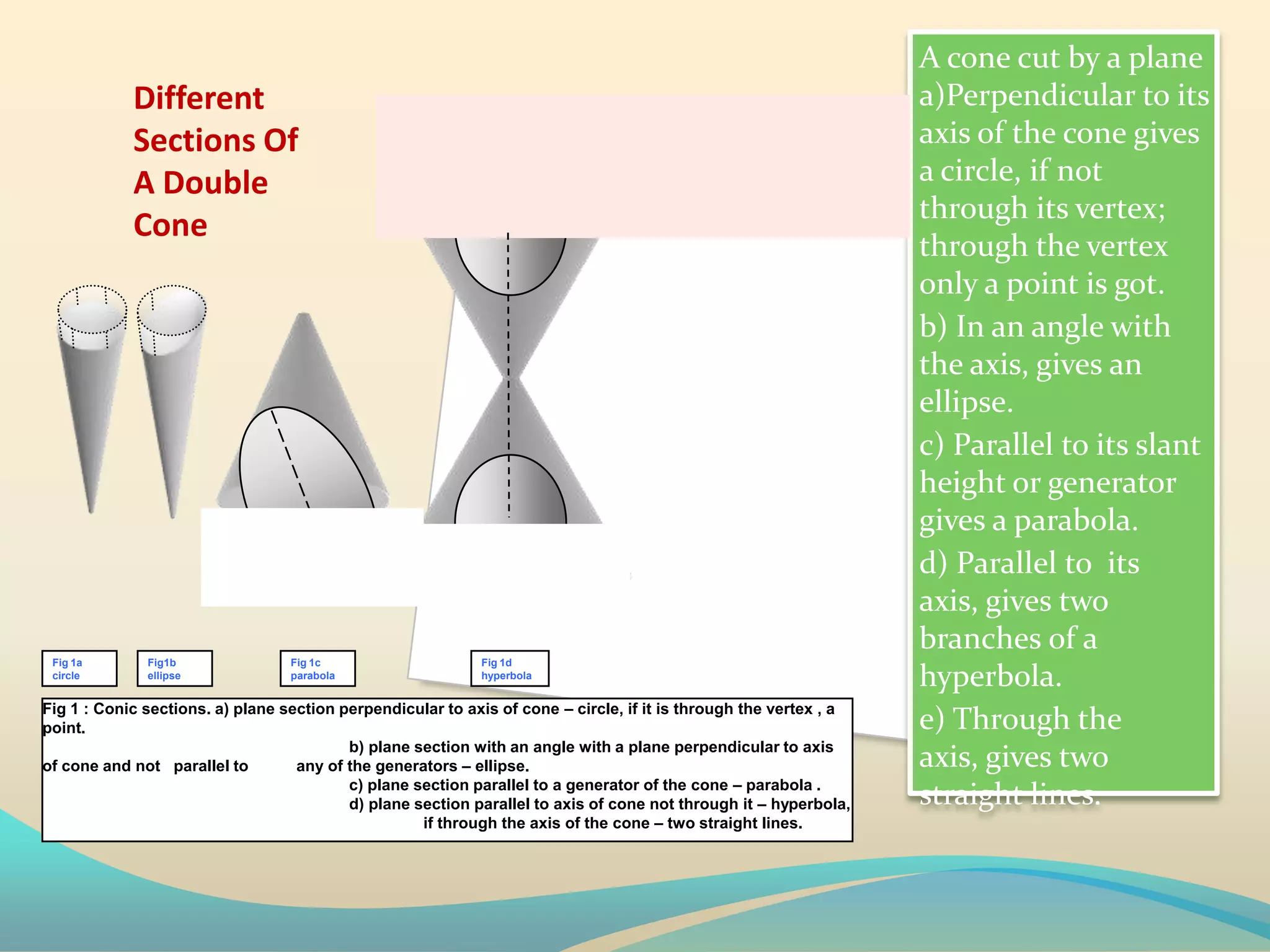
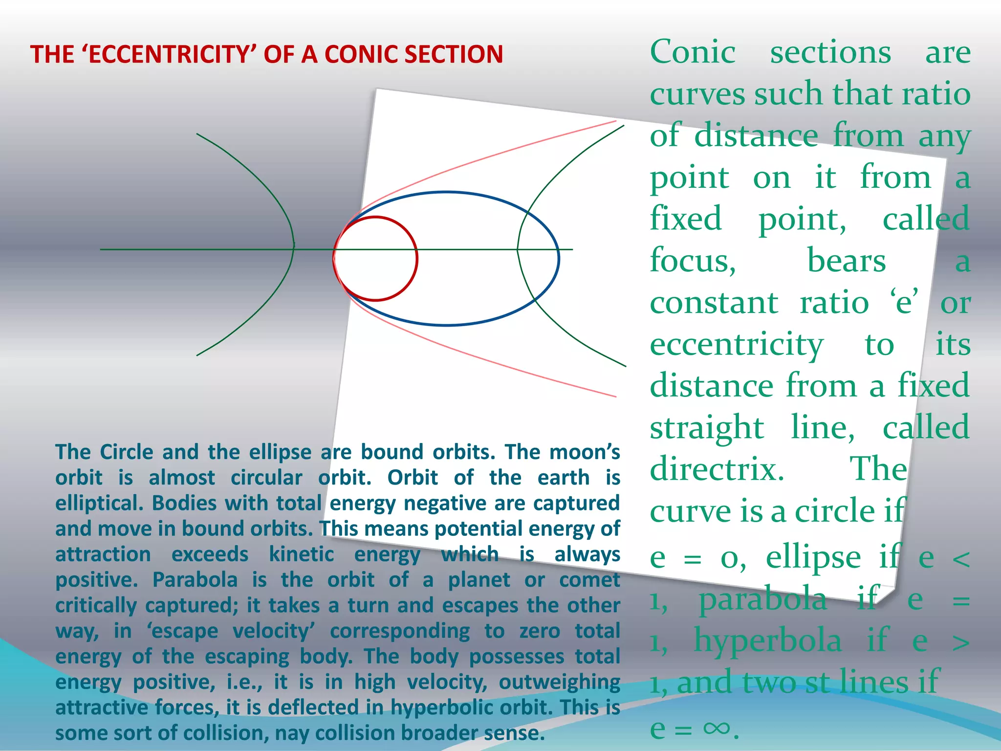
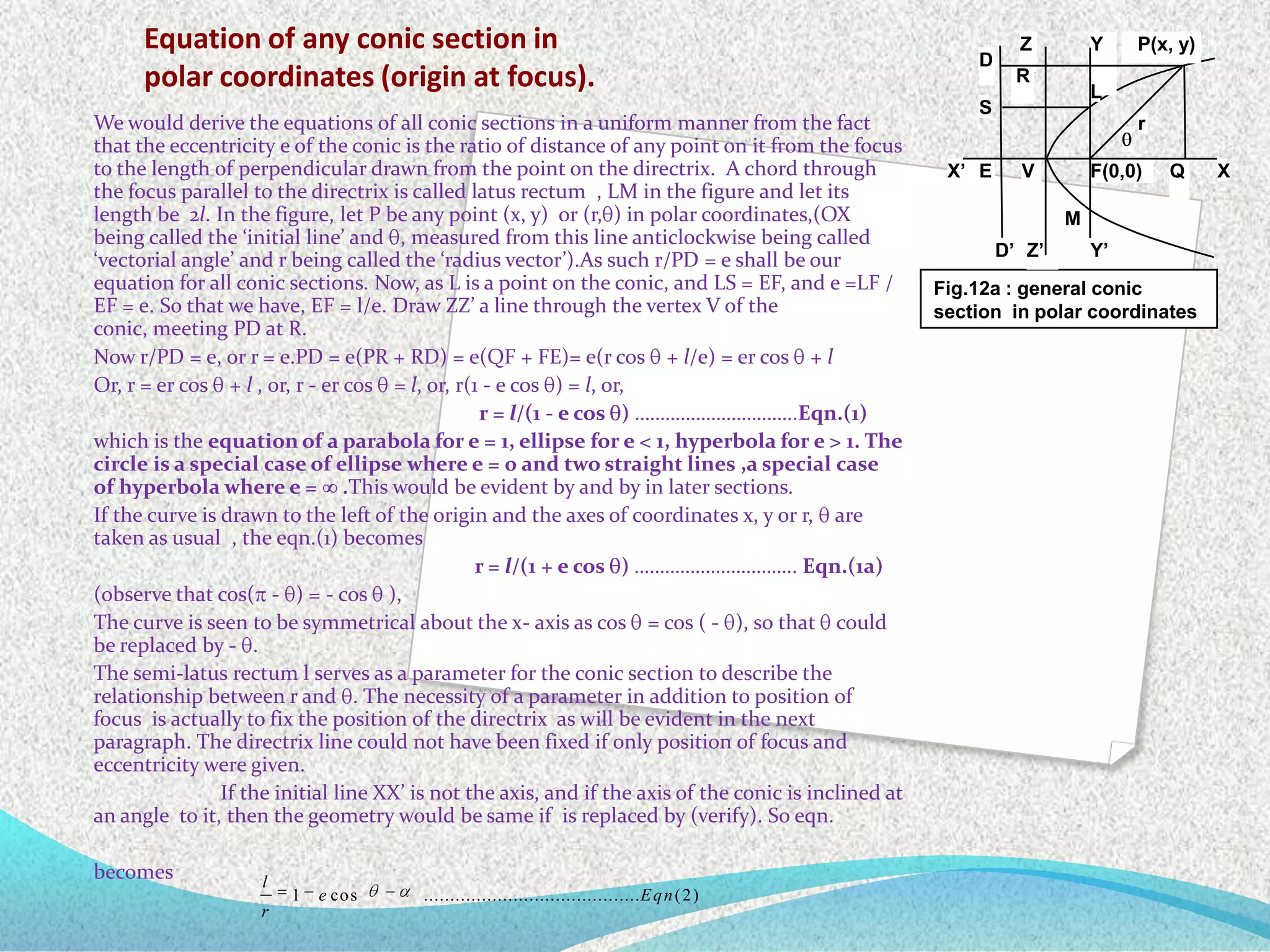
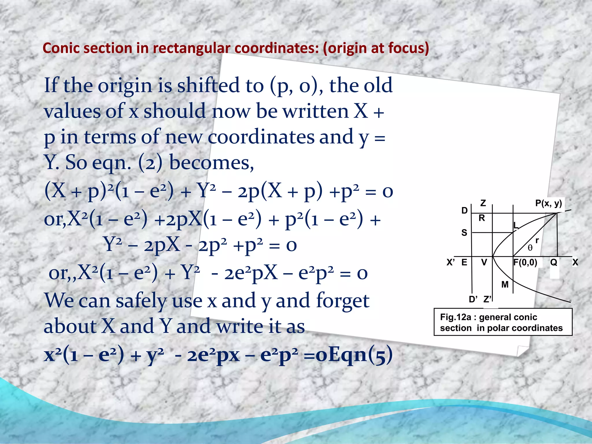
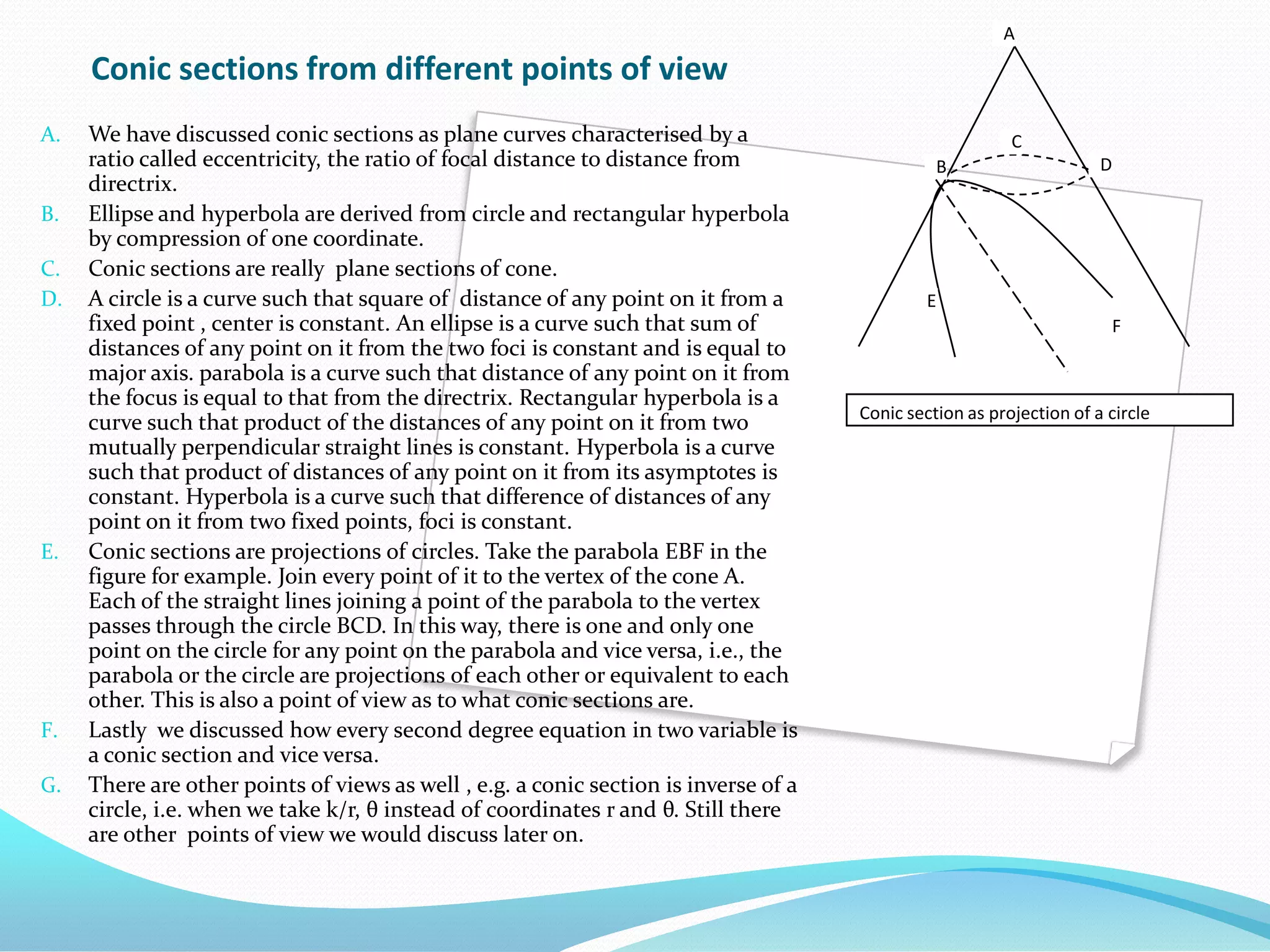
The document discusses conic sections, which are curves formed by the intersection of a cone with a plane. There are four types of conic sections: circles, ellipses, parabolas, and hyperbolas. The document provides equations to define each conic section and explains how the eccentricity relates the distance from a point on the curve to the focus and its perpendicular distance to the directrix. It also presents methods to derive the equations of conic sections in both polar and rectangular coordinate systems with the origin at either the focus or directrix.
The document classifies and describes various solids. Solids are divided into two main groups - Group A solids have bases and tops of the same shape, while Group B solids have a base of one shape and just a point as the top called an apex. Group A includes cylinders and prisms, while Group B includes cones and pyramids. The document then describes the dimensional parameters, sections, and positions of centers of gravity for different solids. It provides steps for solving problems involving solids, including assuming the solid is standing on the relevant plane and drawing multiple views to show the object from different orientations. Finally, it provides examples of specific problems involving drawing the projections of solids in different positions.
1) Hamilton's phase plane provides a clear way to understand how GRIN lenses shape beams and form images by representing the path of rays and phase traces.
2) Key properties like imaging type, magnification, and beam waist position can be directly derived from analyzing the phase traces within and after the lens.
3) This approach provides simpler, more intuitive formulas than traditional matrix methods and gives insights into aberration correction for beam shaping systems.
Here are the steps to solve this problem:
1. Draw the front view of the half cone standing on its half base with the flat face parallel to VP. Show the base diameter and axis length.
2. Draw the top view by projecting the points from the front view.
3. Draw the sectional front view by cutting the half cone with a section plane parallel to both HP and VP, passing through the mid-point of the axis. This will give a semicircular shape.
4. Draw the true shape of the section by drawing a semicircle perpendicular to the section plane at the cut surface. Project cut points onto the true shape and mark distances.
5. Draw the development of the
The document discusses beam profiles of different fiber types and how lenses transform these profiles. It shows that the gradient index multimode fiber beam profile is hyperbolic, similar to the singlemode fiber profile. Geometric optics can accurately describe beam profiles of multimode and singlemode fibers, without needing to consider diffraction effects unless the beam is clipped. The step index multimode fiber beam has two focal waists when focused by a lens, at the image plane and focal plane. Gaussian beam focusing and gradient index multimode fiber beam focusing can be described by similar formulas. The beam profile approach, rather than imaging, is key to understanding beam propagation and focusing properties.
This document classifies and describes various three-dimensional geometric solids. It divides solids into two groups: Group A includes solids with bases and tops of the same shape, such as cylinders and prisms. Group B includes solids with differently shaped bases and tops, specifically cones and pyramids. It provides dimensional parameters and definitions for these solids. The document also describes how to solve problems involving solids through a three-step process and provides examples of specific solid problems involving their projections and orientations in space.
1. The document discusses sectioning of solids by using section planes to cut through objects and understand their internal details. It defines section planes, apparent and true shapes of sections, and provides illustrations of typical section planes and resulting section shapes.
2. Several engineering application problems are provided involving cutting solids like prisms and pyramids with specified section planes and calculating the resulting top views, front views, and true shapes of the sections. Illustrations with steps are given to solve each problem.
3. Readers are instructed to carefully study the illustrations on the next six pages to understand the principles of projections of solids, sections of solids, development, and intersections.
Applied Calculus Chapter 1 polar coordinates and vectorJ C
The document discusses polar coordinates and vectors. It introduces parametric equations to describe the motion of a particle in the xy-plane over time. The variable t is called the parameter. Examples are provided to demonstrate forming Cartesian equations by eliminating t from parametric equations and graphing parametric equations by plugging in values of t. The document also discusses standard representation and finding direction numbers of vectors in R3.
The document provides information on the three conic sections - ellipses, parabolas, and hyperbolas. It defines them as curves that appear on the surface of a cone when cut by different cutting planes. It describes several methods for drawing each type of conic section, such as the concentric circle method for ellipses. It also defines key terms like eccentricity and provides examples of drawing the different conic sections along with normals and tangents to the curves.
This document discusses different types of cones in 3D geometry, including right circular cones and quadratic cones. It provides definitions and properties of cones, as well as theorems regarding their equations. Specifically, it states that the equation of a cone with vertex at the origin is homogeneous of degree 2, and that every homogeneous degree 2 equation represents a cone. It also defines a right circular cone as one generated by lines making a constant angle with the axis, and proves its cross-sections perpendicular to the axis are circles. Finally, it briefly mentions intersections of lines with cones and tangent planes/normals to cones.
This document discusses the four types of conic sections: circles, parabolas, ellipses, and hyperbolas. Each conic section is defined by its geometric properties and standard equation. Examples are given of real-life applications of each conic section, such as circles used in giant wheels and parabolas used in bridges and satellites. The full formulas for all conic sections are also provided.
The document discusses the properties and behavior of light, including reflection, refraction, and how different materials and optical components like lenses interact with light. It explains how lenses can refract light to form real or virtual images, and the factors that determine the type of image formed such as whether the object is between the focal point and lens or beyond it. Different lens shapes and cylindrical lenses are also described.
This document discusses parabolas as a type of conic section. It defines key properties of parabolas including the vertex, focal length, latus rectum, and directrix. The standard and vertex forms of the parabolic equation are presented. Methods for graphing parabolas by plotting points from an equation are described. An example problem calculates the depth of a satellite dish with a parabolic cross-section given its width and the distance to the focus. Real-world applications of parabolas in satellite dishes, heaters, and arched structures are briefly mentioned.
Lecture 2.1.1 Hyperbola is really a section of a conenarayana dash
Hyperbola is really a section of a cone. In early years of student life we were taught that the circle, ellipse, parabola and hyperbola are orbits of planet and satellites and comets. Nobody proved us how. 20 years later, I found the proof in a cremation ground where one of my mothers in law was being cremated. Cremation grounds and burial places are great places for concentration.
Lecture 2.1 shortest derivation of equation of ellipse and meaning of eccentr...narayana dash
1) An ellipse can be obtained by compressing the y-coordinates of a circle by a factor of b/a, where b < a.
2) The eccentricity, e, of an ellipse is defined as the ratio of the distance from the focus (F) to a point on the ellipse and the distance from the directrix to the same point.
3) The sum of the distances from any point on the ellipse to the two foci is equal to the major axis of the ellipse.
Lecture 5.1.5 graphs of quadratic equationsnarayana dash
1) The document discusses graphs of quadratic equations in the form of y = ax^2, y = ax^2 + bx, and y = ax^2 + bx + c.
2) It explains that the graph of y = ax^2 is a parabola that is symmetrical over the y-axis and has a minimum point at the vertex (0,0). The factor a stretches or compresses the graph along the x-axis.
3) Additional terms like b and c shift the graph along the x or y-axis, and the vertex point becomes (-b/2a, c/a - b^2/4a^2) for the equation y = ax^2
Is ellipse really a section of cone. The question intrigued me for 20 odd years after leaving high school. Finally got the proof on a cremation ground. Only thereafter I came to know of Dandelin spheres. But this proof uses only bare basics within the scope of high school course of Analytical geometry.
Lecture 1.16 is parabola really a section of a cone?narayana dash
1) A cone is generated by revolving a line around a fixed line, forming circles where the revolving line intersects planes perpendicular to the fixed line.
2) When a plane cuts through the cone parallel to the plane of the fixed line, the intersection forms the boundary of the surface cut from the cone.
3) The intersection of this cutting plane and the cone can be shown to be a parabola through establishing coordinates and using properties of similar triangles to relate the coordinates.
Lecture 1.6 further graphs and transformations of quadratic equationsnarayana dash
1) The graphs of y2 = x and y2 = -x are parabolas with their axis of symmetry along the x-axis rather than the y-axis.
2) If the coordinate axes are rotated by an angle θ, the equation of a parabola changes but the parabola itself remains the same.
3) Rotating the axes transforms the equation Y = X2 into y cosθ - x sinθ = (x cosθ + y sinθ)2, where θ is the angle of rotation.
The document discusses the differences and relationships between quadratic functions and quadratic equations. It notes that quadratic functions can take any real number as an input, while quadratic equations only have two solutions. The roots of a quadratic equation are also the x-intercepts of the graph of the corresponding quadratic function. The remainder theorem states that the value of a polynomial when a number is substituted for the variable is equal to the remainder when the polynomial is divided by the linear factor corresponding to that number. This connects the roots of quadratic equations to factors of quadratic functions. A quadratic can only have two distinct roots, as having three would mean it has an infinite number of roots.
Lecture 1.3 methods of solutions of quadratic equationsnarayana dash
1. This document discusses four methods for solving quadratic equations: the difficulty-symbol-solution method, completing the square method, using the sum and product of roots, and finding the average of roots.
2. The completing the square method involves adding (b/2a)^2 to both sides of the equation to make the left side a complete square, resulting in the quadratic formula.
3. The sum and product of roots method uses the formulas for the sum (α + β = -b/a) and product (αβ = c/a) of the roots to derive the roots.
4. The average of roots method defines the average of the roots as -b/2a and
Lecture 1.5 graphs of quadratic equationsnarayana dash
1. The document discusses graphs of quadratic equations in various forms such as y = ax^2, y = bx^2 + c, and y = ax^2 + bx + c.
2. Key features of quadratic graphs are discussed, including the vertex, axis of symmetry, maximum/minimum points, and intercepts with the x-axis.
3. Transformations to the graph from changing the coefficients a, b, and c in the equations are explained, such as shifting or stretching the parabola.
Lecture 3.5.1 Ellipse as a compressed circlenarayana dash
1) An ellipse can be obtained by compressing the coordinates of a circle along one axis. If the circle equation is x^2 + y^2 = 1, compressing the y-coordinates by a factor of b/a where b < a yields the ellipse equation (x/a)^2 + (y/b)^2 = 1.
2) The major axis of the ellipse is 2a and the minor axis is 2b. No part of the ellipse lies beyond x = ±a or y = ±b.
3) An ellipse can also be viewed as a circle stretched along one axis, so any ellipse equation can be obtained from a circle by stretching or compressing the coordinates.
1. A central force is one that is always directed towards a fixed point. Examples include gravitational force, forces causing uniform circular motion, and simple harmonic motion.
2. To analyze central forces, vectors, differentiation, and vector differentiation must be understood. The differentiation of position, velocity, and acceleration vectors in Cartesian and polar coordinates is examined.
3. For a central force, the radial component of acceleration is related to the magnitude of the force, while the tangential component depends on the angular acceleration and velocity. Examples of central forces producing different types of motion are given.
This slide is special for master students (MIBS & MIFB) in UUM. Also useful for readers who are interested in the topic of contemporary Islamic banking.
How to Setup Warehouse & Location in Odoo 17 InventoryCeline George
In this slide, we'll explore how to set up warehouses and locations in Odoo 17 Inventory. This will help us manage our stock effectively, track inventory levels, and streamline warehouse operations.
This presentation includes basic of PCOS their pathology and treatment and also Ayurveda correlation of PCOS and Ayurvedic line of treatment mentioned in classics.
A review of the growth of the Israel Genealogy Research Association Database Collection for the last 12 months. Our collection is now passed the 3 million mark and still growing. See which archives have contributed the most. See the different types of records we have, and which years have had records added. You can also see what we have for the future.
Chapter wise All Notes of First year Basic Civil Engineering.pptxDenish Jangid
Chapter wise All Notes of First year Basic Civil Engineering
Syllabus
Chapter-1
Introduction to objective, scope and outcome the subject
Chapter 2
Introduction: Scope and Specialization of Civil Engineering, Role of civil Engineer in Society, Impact of infrastructural development on economy of country.
Chapter 3
Surveying: Object Principles & Types of Surveying; Site Plans, Plans & Maps; Scales & Unit of different Measurements.
Linear Measurements: Instruments used. Linear Measurement by Tape, Ranging out Survey Lines and overcoming Obstructions; Measurements on sloping ground; Tape corrections, conventional symbols. Angular Measurements: Instruments used; Introduction to Compass Surveying, Bearings and Longitude & Latitude of a Line, Introduction to total station.
Levelling: Instrument used Object of levelling, Methods of levelling in brief, and Contour maps.
Chapter 4
Buildings: Selection of site for Buildings, Layout of Building Plan, Types of buildings, Plinth area, carpet area, floor space index, Introduction to building byelaws, concept of sun light & ventilation. Components of Buildings & their functions, Basic concept of R.C.C., Introduction to types of foundation
Chapter 5
Transportation: Introduction to Transportation Engineering; Traffic and Road Safety: Types and Characteristics of Various Modes of Transportation; Various Road Traffic Signs, Causes of Accidents and Road Safety Measures.
Chapter 6
Environmental Engineering: Environmental Pollution, Environmental Acts and Regulations, Functional Concepts of Ecology, Basics of Species, Biodiversity, Ecosystem, Hydrological Cycle; Chemical Cycles: Carbon, Nitrogen & Phosphorus; Energy Flow in Ecosystems.
Water Pollution: Water Quality standards, Introduction to Treatment & Disposal of Waste Water. Reuse and Saving of Water, Rain Water Harvesting. Solid Waste Management: Classification of Solid Waste, Collection, Transportation and Disposal of Solid. Recycling of Solid Waste: Energy Recovery, Sanitary Landfill, On-Site Sanitation. Air & Noise Pollution: Primary and Secondary air pollutants, Harmful effects of Air Pollution, Control of Air Pollution. . Noise Pollution Harmful Effects of noise pollution, control of noise pollution, Global warming & Climate Change, Ozone depletion, Greenhouse effect
Text Books:
1. Palancharmy, Basic Civil Engineering, McGraw Hill publishers.
2. Satheesh Gopi, Basic Civil Engineering, Pearson Publishers.
3. Ketki Rangwala Dalal, Essentials of Civil Engineering, Charotar Publishing House.
4. BCP, Surveying volume 1
it describes the bony anatomy including the femoral head , acetabulum, labrum . also discusses the capsule , ligaments . muscle that act on the hip joint and the range of motion are outlined. factors affecting hip joint stability and weight transmission through the joint are summarized.
Walmart Business+ and Spark Good for Nonprofits.pdfTechSoup
"Learn about all the ways Walmart supports nonprofit organizations.
You will hear from Liz Willett, the Head of Nonprofits, and hear about what Walmart is doing to help nonprofits, including Walmart Business and Spark Good. Walmart Business+ is a new offer for nonprofits that offers discounts and also streamlines nonprofits order and expense tracking, saving time and money.
The webinar may also give some examples on how nonprofits can best leverage Walmart Business+.
The event will cover the following::
Walmart Business + (https://business.walmart.com/plus) is a new shopping experience for nonprofits, schools, and local business customers that connects an exclusive online shopping experience to stores. Benefits include free delivery and shipping, a 'Spend Analytics” feature, special discounts, deals and tax-exempt shopping.
Special TechSoup offer for a free 180 days membership, and up to $150 in discounts on eligible orders.
Spark Good (walmart.com/sparkgood) is a charitable platform that enables nonprofits to receive donations directly from customers and associates.
Answers about how you can do more with Walmart!"
1. Paths of planets, satellites and comets are
beautiful curves called conic sections. They
are obtained when a cone is intersected by a
plane surface.
And also they have many other
beautiful and interesting facts about them.
For example they are such curves that
distance from any point on the curve from a
fixed point bears a constant ratio to distance
from a fixed st line.
2. A cone cut by a plane
a)Perpendicular to its
Different
axis of the cone gives
Sections Of
a circle, if not
A Double
through its vertex;
Cone
through the vertex
only a point is got.
b) In an angle with
the axis, gives an
ellipse.
c) Parallel to its slant
height or generator
gives a parabola.
d) Parallel to its
axis, gives two
branches of a
Fig 1a Fig1b Fig 1c Fig 1d
hyperbola.
circle ellipse parabola hyperbola
Fig 1 : Conic sections. a) plane section perpendicular to axis of cone – circle, if it is through the vertex , a
e) Through the
point.
b) plane section with an angle with a plane perpendicular to axis
axis, gives two
any of the generators – ellipse.
of cone and not parallel to
c) plane section parallel to a generator of the cone – parabola .
straight lines.
d) plane section parallel to axis of cone not through it – hyperbola,
if through the axis of the cone – two straight lines.
3. We know the axis of earth always
The pole star
ORBIT OF points towards the pole star. In fact
that is the reason of changing seasons.
THE EARTH
If every point of the orbit is joined to
the pole star, we get a cone ; not an odd
shaped one, but a round smooth one
called a right circular cone.
Again the Sun is not placed at its
center; but a t point called its focus, far
away from the center.
Planets and satellites move in elliptical
orbits
Comets who are seen periodically
move around the Sun in vey long
elliptical orbits.
The Earth
Some travelling comets at high speed
are not captured by the Sun, they just
bend around it once and pass away in
parabolic orbits.
Still some comets are in so high speed
that they are deflected back from the
Sun and turn away in hyperbolic
orbits. This is some sort of collision.
The Sun
4. Conic sections are
THE ‘ECCENTRICITY’ OF A CONIC SECTION
curves such that ratio
of distance from any
point on it from a
fixed point, called
focus, bears a
constant ratio ‘e’ or
eccentricity to its
distance from a fixed
straight line, called
The Circle and the ellipse are bound orbits. The moon’s
directrix. The
orbit is almost circular orbit. Orbit of the earth is
elliptical. Bodies with total energy negative are captured curve is a circle if
and move in bound orbits. This means potential energy of
e = 0, ellipse if e <
attraction exceeds kinetic energy which is always
positive. Parabola is the orbit of a planet or comet
1, parabola if e =
critically captured; it takes a turn and escapes the other
way, in ‘escape velocity’ corresponding to zero total
1, hyperbola if e >
energy of the escaping body. The body possesses total
1, and two st lines if
energy positive, i.e., it is in high velocity, outweighing
attractive forces, it is deflected in hyperbolic orbit. This is
e = ∞.
some sort of collision, nay collision broader sense.
5. Equation of an ellipse
Y
2 2
x y
1
2 2
a a
P
a
Q (x y)
O
X’ X
M b R N
2
2
y
x
1 2
2
2 2 y
x
a b 1
2 2
Y’ b b
2 2
Let the eqn. of the circle be written in form ……………………………………..………….(a)
X Y
1
2 2
a a
Transform the coordinates to x and y ,only by compressing Y coordinates by a factor b/a
where b/a < 1;i.e.,x = X, and y = b .Y/a ; OR X = x and Y = a .y/b.………………………………….(b)
The curve PMN is now changed to the curve QMN because of the transformation of coordinates
to new coordinates x and y. A relationship between x and y shall be its equation. Since x and y are
related to X and Y as in (b) and X and Y are related to each other as in (a), we can rewrite (a) as,
2
2
ay 2 2
x y
2
x 2
b 1
1 2 2
a b
2 2
a a
which is the only one relationship between x and y we sought for, and becomes the eqn. of the
new curve ( called ellipse).
6. A meaning Of eccentricity ‘e’
The circle has a centre and the ellipse has also a centre. But
the centre of the ellipse is not that important as the centre of
the circle. The ellipse has no such radial symmetry as in the
case of circle. Instead, there are two other points of importance
along the main axis or the major axis , one on each side of the
center , each being called a focus. How far the focus is moved
from the center so that the circle is flattened to become an
ellipse is measured by its eccentricity. We explore below how
the focus and eccentricity are related .
In the eqn.of the ellipse , put b = fa or b/a = f, (evidently f <
1, as b < a). This reduces the eqn tox2f2 + y2 =
a2f2…………….(a)
The left side looks like square of a distance (as we
knew distance formula between the points (x, y) and (x1, y1), d
=√{(x- x1) 2+ (y- y1) 2} and the form of the equation indicates us
to make the expression a complete square so as to see what
distance it might be. Put e2 = 1 – f2 (certainly we can, as f < 1)
so that x2f2 becomes
x2 (1 – e2 ), and a2f2 becomes a2 (1 – e2 ), Thus the eqn.
becomes
x2 + a2e2 + y2 = a2 + e2x2
In further endeavour to complete squares, we add – 2aex to
both sides and get (x – ae)2 + (y – 0)2 = e2(x – a/e)2………..(b)
7. Spokes of a wheel being pulled by two
Visualisation of e rods called directrices; the center splits
into two points moved away from each
other called foci.
8. The sum of focal distances from any point on the
ellipse = 2a, the major axis.
Choose the origin midway between the
two fixed points and choose the x-axis
along the line joining the two fixed
points. There is no loss of generality as
we can shift the origin and the axes later
as we please. Thus the coordinates of
the two fixed points may be taken as
(k, 0) and ( - k, 0) ; or as (ae, 0) and
( - ae, 0) if we denote k /a = e. Later on
we would observe that this is really the
eccentricity e. If (x, y) be the
coordinates of the point , the sum of
whose distances from (ae, 0) and
( - ae, 0) is 2a; we have, the steps are:
( x ae ), y
2 2 2 2
( x ae ) y 2a
2 2 2 2 2 2 2 2 2
2x 2a e 2y 2 (x ae ) y (x ae ) y 4a
2
2 2
2 2 2 2 2 2 2 2 2 2 2 2
x ae y 2a x ae y 4x a e
2 2 2 2
x y x y
1 1
2 2 2 2 2
2 2 2 2 2 2 2
a a (1 e) a b
a xe x ae y
9. Equation of any conic section in Z Y P(x, y)
D
polar coordinates (origin at focus). R
L
S
We would derive the equations of all conic sections in a uniform manner from the fact r
that the eccentricity e of the conic is the ratio of distance of any point on it from the focus
to the length of perpendicular drawn from the point on the directrix. A chord through X’ E V F(0,0) Q X
the focus parallel to the directrix is called latus rectum , LM in the figure and let its
length be 2l. In the figure, let P be any point (x, y) or (r, ) in polar coordinates,(OX M
being called the ‘initial line’ and , measured from this line anticlockwise being called
D’ Z’ Y’
‘vectorial angle’ and r being called the ‘radius vector’).As such r/PD = e shall be our
equation for all conic sections. Now, as L is a point on the conic, and LS = EF, and e =LF / Fig.12a : general conic
EF = e. So that we have, EF = l/e. Draw ZZ’ a line through the vertex V of the section in polar coordinates
conic, meeting PD at R.
Now r/PD = e, or r = e.PD = e(PR + RD) = e(QF + FE)= e(r cos + l/e) = er cos + l
Or, r = er cos + l , or, r - er cos = l, or, r(1 - e cos ) = l, or,
r = l/(1 - e cos ) …………………………..Eqn.(1)
which is the equation of a parabola for e = 1, ellipse for e < 1, hyperbola for e > 1. The
circle is a special case of ellipse where e = 0 and two straight lines ,a special case
of hyperbola where e = .This would be evident by and by in later sections.
If the curve is drawn to the left of the origin and the axes of coordinates x, y or r, are
taken as usual , the eqn.(1) becomes
r = l/(1 + e cos ) ………………………….. Eqn.(1a)
(observe that cos( - ) = - cos ),
The curve is seen to be symmetrical about the x- axis as cos = cos ( - ), so that could
be replaced by - .
The semi-latus rectum l serves as a parameter for the conic section to describe the
relationship between r and . The necessity of a parameter in addition to position of
focus is actually to fix the position of the directrix as will be evident in the next
paragraph. The directrix line could not have been fixed if only position of focus and
eccentricity were given.
If the initial line XX’ is not the axis, and if the axis of the conic is inclined at
an angle to it, then the geometry would be same if is replaced by (verify). So eqn.
becomes l
1 e co s ......................................... E q n (2 )
r
10. Conic section in rectangular coordinates: (origin at directrix)
In rectangular coordinates, (see fig.12a ) , taking the directrix, DD’ as
the y-axis, and taking the distance of the focus at a distance p from
it, i.e., EF = p, and PD = EQ =x, we have,
PF2 /PD2 = e2 , PF2 = PD2e2 = e2x2, PF2 = FQ2 + PQ2 =
(EQ – EF)2 + PQ2 =(x – p )2 + y2,
(x – p )2 + y2 = e2x2, p being called the focal parameter, being
Or,
the distance from the focus to the directrix.
Z P(x, y)
x2(1 – e2) + y2 – 2px +p2 = 0……………………Eqn.(3). D R
Or,
L
As FL = eSL = eEF, where FL = l and EF = p, S
r
we have l = pe………………………………………………. Eqn.(4) X’ E V F(0,0) Q X
Semi-latus rectum = pe. M
D’ Z’
Fig.12a : general conic
section in polar coordinates
11. Conic section in rectangular coordinates: (origin at focus)
If the origin is shifted to (p, 0), the old
values of x should now be written X +
p in terms of new coordinates and y =
Y. So eqn. (2) becomes,
(X + p)2(1 – e2) + Y2 – 2p(X + p) +p2 = 0 Z P(x, y)
D
or,X2(1 – e2) +2pX(1 – e2) + p2(1 – e2) + R
L
S
Y2 – 2pX - 2p2 +p2 = 0 r
X’ E V F(0,0) Q X
or,,X2(1 – e2) + Y2 - 2e2pX – e2p2 = 0 M
We can safely use x and y and forget D’ Z’
Fig.12a : general conic
about X and Y and write it as section in polar coordinates
x2(1 – e2) + y2 - 2e2px – e2p2 =0Eqn(5)
12. Conic section in rectangular coordinates: (origin at any point in general)
…………………………………………………… eqn(6)
2
( Ax By C)
2 2 2
( x - h) (y k) e 2 2
A B
Is the equation of general conic section including circle, ellipse, parabola and
hyperbola according as
e = 0, e < 1, e =1, and e > 1. Focus is the point (h, k) and directrix is the st. line . The
cases would be clear in the appropriate sections.
Let the point V be the vertex at the origin (0, 0) and let the directrix DD’ be at a
distance a , i.e., at the point G ( - a, 0). If the focus is at F, VF/VG = e, as VG = a,
VF must be ae, so that F is at (ae, 0). If P(x, y) be any point on the conic, PF/PD =
e, If PD cuts y-axis at R, or, PF/(PR +RD) = e, or, PF/(PR +VG) = e, or, PF/(VQ +VG)
= e, or, r/(x + a) = e,
From here we can go to r/(r cos + a ) = e, ………………………………eqn.(7)
Or, ……………………………………………………………...eqn.(8)
2 2
x y /(x + a) = e
so , or …………………………………………………………………………..eqn(9)
2 2 2 2
x y =e (x + a)
Or ………………………………………………………………eqn(10)
2 2 2 2 2
x (1 e ) 2 aex e a y =0
This ‘a’ must not be confused with semi major axis of the ellipse.
Here it is the distance of the directrix from the vertex. Now l = LF =
eSL = e(FV + VG) = e(ae +a);so a e l a e …………………………..eqn(11)
13. Derivation of Eqn of Ellipse in Cartesian Coordinates
The eqn. for general conic x2(1 – e2) + y2 – 2px +p2 = 0 becomes,
x2(1 – e2) + y2 – 2 (a/e – ae )x +(a/e – ae)2 = 0 .
which is the equation of the ellipse. with origin
at the directrix and focus at (a/e – ae,0).
For, we already know that distance of the directrix of ellipse from its center is a/e , and
distance of the focus from the center is ae. So p = a/e – ae.
Only we have to shift the origin a/e to the right, i.e., replace x by x+ a/e
So the eqn. taking origin at the centre of ellipse this eqn becomes,
(x+ a/e)2(1 – e2) + y2 – 2 (a/e – ae )( x+ a/e) +(a/e – ae)2 = 0
or, x2(1–e2)+y2 –2(a/e–ae)(x +a/e)+(a/e–ae)2+2x(a/e)(1– e2)+(a/e)2(1–e2) = 0
or, x2(1–e2)+y2 –2(a/e–ae)x–2(a/e–ae) a/e+(a/e–ae)2+
2x(a/e– ae)+ (a/e)2(1–e2) = 0
or, x2(1–e2)+y2 – 2(a/e)2(1 – e2) +(a/e–ae)2 +(a/e)2(1–e2) = 0
or, x2(1–e2)+y2– (a/e)2(1 – e2) +(a/e–ae)2 = 0 ,
or, x2(1–e2)+y2– (a/e)2(1 – e2) +(a/e)2(1-e2)2 = 0
or, x2(1–e2)+y2 - (a/e)2(1–e2) + (a/e)2(1-2e2 +e4) = 0
or, x2(1–e2)+y2 - (a/e)2(1–e2 - 1+ 2e2 - e4) = 0
or, x2(1–e2)+y2 - (a/e)2e2(1 –e2) = 0 , or, x2(1–e2)+y2 – a2(1 –e2) = 0
or, , as before; or where as before.
2 2
x y 2 2 2
b a 1 e
1
2 2 2
a a 1 e
14. Z P(x, y)
D
Equation of parabola R
L
S
r
This is an example of how we derive equations of conic X’ E V(0, 0) F Q X
section from focus directrix definition from the first M
principles. D’ Z’
In the above figure and with the labels as before, A parabola Fig.12a : general conic
section in polar coordinates
is the curve such that any point on this curve, P(x, y) is at
the same distance from the focus F as the distance from the
directrix, PD. So PF = PD = QE.
Next, if V(0, 0) is a point on the parabola, called its
vertex, then , by above definition, VE = VF. Let us call VE =
a, so that F is the point (a,0). Now, PF2 = r2 = FQ2 +QP2 =
(x-a)2 +y2. Again PD2 = PR2 + RD2=(x+a) 2
Thus , or y2 = 4ax …………………………… ………..eqn(12)
It the origin is transferred to the point ( - a , 0), or it is
taken to the directrix, then x should be replaced by x – a
, so that the equation to the parabola becomes,
y2 = 4a(x – a)…………………………. eqn(13a)
It the origin is transferred to the point focus, ( a , 0), then x
should be replaced by
x + a , so that the equation to the parabola becomes,
2
15. Equation of rectangular hyperbola
YA
R
In the figure, APB be a curve where P(x, y) is any point on R P(x, y)
it such that OQ = x = RP and PQ = y = RO; and
B
xy = c2…………………..……………………..Eqn(14a) X’
O Q X
Such a curve is called a rectangular hyperbola A’
characterized by the feature that the product of its P’
distances from two fixed st.lines at right angles to each y= - x
R’
other , the coordinate axes in the present case is a positive B’ Y’
constant say c2. The curve has two branches APB and Fig.16, rectangular hyperbola
A’P’B’ in the first and third quadrants If we move further
to the right of any point P (x, y) the y- coordinate
decreases and the x- coordinate increases in the inverse
proportion so that xy remains constant. Down along the
x- axis, the y- coordinate diminishes to 0 at large distance
, so that the x- axis touches the curve at ∞. Similarly the
curve touches the y – axis at ∞. A line touching a curve at
∞ is called an asymptote of the curve. Further, the
branch A’P’B’ is reflection of the branch APB , not about
any axis, but about the line y = - x shown as a dotted line.
The fact may be verified by observing that the equation of
this curve is unchanged by replacing x, y by – x and – y
respectively. Further, it may be noted that the curve is
symmetric about the line y = x , for interchanging x and y
in the eqn makes no difference.
16. Equation of rectangular hyperbola YA
R
R P(x, y)
An analogy with the circle:
In an ellipse, the sum of distances of any point on it is B
constant and equal to its major axis. Similarly, on this curve, X’
O Q X
the rectangular hyperbola, product of distances from two A’
fixed st.lines is constant. ( its distance from y –axis being x P’
and the distance from x – axis being y). y= - x
R’
The curve can be transformed by a change of axes , the new B’ Y’
axes got from rotating the existing axes by 450 anticlockwise. Fig.16, rectangular hyperbola
The new set of axes, say X and Y form another rectangular
Cartesian coordinate system about the same origin. If new
coordinates of P be (X, Y) , we have, from principle of
transformation of coordinates,
x = X cos 450 – Y sin 450 and y = X sin 450 + Y cos450………….(b)
Putting the values in (a),
(X cos 450 – Y sin 450)( X sin 450 + Y cos 450) = c2
(X / 2 – Y / 2)( X / 2 + Y / 2) = c2
or,
X2 – Y2 = 2c2
or
X2 – Y2 = a2
or,
2 2
X Y
1
or, …………………..………………………….(14)
2 2
a a
17. Equation of hyperbola
Now the technique of compressing Y-
D2 Y D1 L
coordinate may be applied. Let all Y- P’
M P
coordinates be compressed in the ratio M’
b b
;so y’= a Y, and x’ = X. Thus the eqn.
a
F’ F
2 2
reduces to x' y'
1
X’ A’ N’ O N A Q X
2 2
a b
which may be re-written in usual form ,
for the only reason of sheer convenience
2 2
as, x y 1 ……………… Eqn.(15) Q’ D2’ D1’ Q
Y’ L’
2 2
a b
We also can arrive at the ratio of Fig. 17 : Hyperbola
focal distance to the directory
distance of a point just in the
manner we did for the ellipse.
which can be regarded as the standard
equation of a hyperbola. Just as the
eqn. of ellipse is derived from the eqn.
of a circle, the eqn. of hyperbola is
derived from eqn. of a rectangular
hyperbola in the same manner. Hence
the rectangular hyperbola may be
considered as a counterpart of a circle.
18. L’
Y X
N’ S’
TO SHOW THAT AN HYPERBOLA IS T’
ACTUALLY A SECTION OF A CONE
Let a st.line VU revolve around a fixed M’
st.line VG making a constant angle with a
it at V and generate a double cone as V C(0, 0)
b
shown in the figure. Let a plane parallel L
a
to VG and perpendicular to the plane of L
M
VUW cut the double cone in a curve in x
two branches LMN and L’M’N’ , M and x
P
M’ being two points on the cone. Let VC y
= b , be perpendicular to MM’. Set up a 900 Y’
S T
rectangular Cartesian coordinate r O b R
L
system at C , midpoint of M’M and MM’ U W
being the x-axis and YY’ being y-axis in N
the intersecting plane. Take any point P
on the curve of intersection and draw a X’
L
G
perpendicular PR onto MM’ and extend L
Fig. 18 : A hyperbola is really a section of a cone
it until it meets the curve at N.
Coordinates of the point P are x = CR
and y = PR. Take a plane containing PR
and perpendicular to the plane VST .
this plane intersects the cone in a circle
PST having its centre at O and radius
OP = OS = OT = r.
19. L’
Y X
N’ S’
L
TO SHOW THAT AN HYPERBOLA IS T’
ACTUALLY A SECTION OF A CONE
This can be proved from M’
a
congruence of the two triangles V C(0, 0)
b L
VSO and VOT, having the side a
L
M
VO common, and two equal x
angles SVO = = OVT and x
P
L
y
having a right angle each. OVCR 900 Y’
S T
r O b R
can be proved to be a rectangle U W
as three of its angles are right N
angles, so that OR = VC = b. X’
L
G
Now PR is in the intersecting L
Fig. 18 : A hyperbola is really a section of a cone
plane and OR is in the plane of
the circle PST and the two
planes are perpendicular to each
other. So OR PR and it follows
that OP2 = OR2 + PR2.
Or, r2 = b2 + y2…………………….(a)
20. Continued from the previous slide
As OP = r, OR = b and PR = y..
The relationship between x and y shall be the eqn. to the curve of
intersection we require, which can be obtained from this eqn.(a) r in terms
of x. We immediately observe that r = OS = OV tan and OV = CR = x.
x2tan2 = b2 + y2………………………………...(b)
Hence we get,
is the required equation to the curve of intersection. If we denote
the length CM = a, observe that CMV = MVO = , so that tan = b/a.
x2b2 = a 2b2 + a2y2 or,
Now eqn. (b) becomes,
…………….( c)
2 2
x y
1
2 2
a b
which is standard equation to a hyperbola . Note that ‘a’ is actually seen to
be its semi-major axis and ‘b’ is equal to its semi-minor axis, though it is not
in the plane of the curve. The value of e may be obtained from ,
…………………………………(d)
2
b
2 2 2
e 1 1 tan sec
2
a
which is always greater than 1 for any given acute angle . For a different
value of e we need a different value of , or in other words, need a different
cone altogether. From one cone, we get hyperbolas all of same e value
i.e., sec2 . This is because either we have to choose a different cone or
different values of a and b; to get different hyperbolas from the same
cone, i.e., the plane of intersection must be different.
21. Continued from the previous slide
This is a meaning of e for the hyperbola.
2 2 2 2
x y x y
It may be further noted that in the eqn. of an ellipse a a (1 e ) ,or a b 1
1
2 2 2 2 2
, where , e is supposed to be less than 1, i.e., b < a. If we make e > 1
2 2 2
b a (1 e )
, e becomes imaginary and we do not get a hyperbola in place of an ellipse, as b
2 2
becomes imaginary; not evenif we rewrite the same equation as . x y
1
2 2 2
a a (e 1)
On the other hand, if we make b > a in , we get only another ellipse with its
major and minor axes interchanged. 2 2
x y
1
The hyperbola shown in the figure of this article is represented by ; a b 2 2
where b is the length of the perpendicular from vertex of the cone onto the plane
of intersection , i.e., onto the plane of the hyperbola. But as it is the standard
eqn. of hyperbola, b is supposed to be less than a , and it is very much the semi-
minor axis, which is supposed to be in the plane of the hyperbola. Thus the
length of the perpendicular from vertex of the cone happens to be equal to the
semi-minor axis, the two being perpendicular to each other. This is as if the
minor axis has been rotated through /2 or having been multiplied by i = (-1)
, perhaps because b2 in the equation of the ellipse is replaced by - b2 in contrast
to the case of ellipse. Then e 1 b 1 tan which is always greater than 1.
2
2 2 2
sec
2
a
22. The general eqn. of 2nd degree in two variables represents a conic.
The General eqn. of 2nd degree ax2 +2hxy + by2 + 2gx +2fy +c = 0……….…eqn(16)
By a suitable transformation of co-ordinates , the xy-term may be made to vanish.
Suppose the axes are turned through an angle so that, x is replaced by
x cos -y sin and y is replaced by x sin + y cos ,so that (16) becomes
a(x cos - y sin )2 + 2h(x cos - y sin )( x sin + y cos )+ b(x sin
+ y cos )2+2g(x cos - y sin ) + 2f(x sin + y cos ) + c = 0.
The coefficient of 2xy term is h(cos2 -sin2 ) – (a – b) cos sin ,which is 0 if,
2h cos 2 = (a – b) sin 2 , or tan 2 = 2h/(a – b).
For any real value of h, a and b, can always be found, so that the eqn. can always
be got rid of the xy-term (second term).Even for a = b, cos 2 = 0 and = /4 if we
put a = b from the beginning. And thus can be written in the form
Ax2 +By2 + 2Gx +2Fy +C = 0…………………………………………………………….(17)
Of course c = C as the term does not involve the variables only whom we have
modified. Thus we can take (17) as general equation of second degree in two
variables without any loss of generality.
This equation can be written as follows by completing squares
……………………………………...(18)
2 2 2 2
G F G F
Ax By C K ( sa y )
2 2
A B A B
if A 0 and B 0.
23. The general eqn. of 2nd degree in two variables represents a conic.
If the origin is shifted to the point , eqn.(17) can be written as
G F
,
A B
, ..................................... (18)
2 2
x y
1
K K
A B
(to keep the number of symbols minimum, we write x and y instead of new
symbols, though x and y in (18) are different from x and y in (17)or simply transfer
the origin to )
G F
,
A B
The eqn. represents an ellipse , real if K/A and K/B both are positive, or
imaginary one , if K/A and K/B both are negative, their roots are imaginary.
This shows that a second degree eqn in two variables Ax2 +By2 + 2Gx +2Fy +C = 0
in which there is no xy-term shall be equation of an ellipse if A and B are of
2 2
same sign as that of . G F C 2 2
A B
Eqn.(18) represents a hyperbola if one of K/A and K/B is negative.
This shows that a second degree eqn in two variables Ax2 +By2 + 2Gx +2Fy +C = 0
in which there is no xy-term shall be equation of an hyperbola if A and B are of
opposite signs.
24. The general eqn. of 2nd degree in two variables represents a conic.
2
C F F
If A = B, this represents a circle , origin at and radius
,
2G 2 B G B
………………...(19)
K K
or
A B
and only a point , trivial case of circle if K = 0.
If one of A, B, is 0 , say A = 0 and B 0, from eqn.(18) we get,
By2 + 2Gx +2Fy +C = 0……………………………………………..…..(20)
Do not put A = 0 direct in that equation.
By completing the square, 2 2
F C F
By 2G x 0
B 2G 2 BG
Or, By2 +2Gx = 0 or, 2G
……………………………………..(21)
2
y x
B
which represents a parabola if the origin is shifted to
its branches towards negative side of the x-axis if G/A is positive and vice versa.
If G = 0 along with A = 0, from eqn.(17) we get,
In other words, a second degree eqn in two variables
Ax2 +By2 + 2Gx +2Fy +C = 0 in which there is no xy-term shall be
equation of a parabola, if A = 0 , G 0.
2
By2 + 2Fy + C = 0 or y F F B C ………………………………………….(22)
B
which represents two straight lines parallel to each other and parallel to x-axis. The
25. The general conic represents the following curves
under respective conditions.
Summary
What curve Under what condition
Ellipse 2
h ab
Parabola 2
h ab
Hyperbola
2
h ab
Circle a = b and h =0
Rectangular hyperbola a + b =0
Δ =0, where Δ =abc +2fgh – af2 – bg2 – ch2
Two st lines, real or imaginary
Δ =0 and
Two parallel st lines 2
h ab
26. A
Conic sections from different points of view
We have discussed conic sections as plane curves characterised by a
A. C
ratio called eccentricity, the ratio of focal distance to distance from D
B
directrix.
Ellipse and hyperbola are derived from circle and rectangular hyperbola
B.
by compression of one coordinate.
Conic sections are really plane sections of cone.
C.
A circle is a curve such that square of distance of any point on it from a
D. E
fixed point , center is constant. An ellipse is a curve such that sum of F
distances of any point on it from the two foci is constant and is equal to
major axis. parabola is a curve such that distance of any point on it from
the focus is equal to that from the directrix. Rectangular hyperbola is a
Conic section as projection of a circle
curve such that product of the distances of any point on it from two
mutually perpendicular straight lines is constant. Hyperbola is a curve
such that product of distances of any point on it from its asymptotes is
constant. Hyperbola is a curve such that difference of distances of any
point on it from two fixed points, foci is constant.
Conic sections are projections of circles. Take the parabola EBF in the
E.
figure for example. Join every point of it to the vertex of the cone A.
Each of the straight lines joining a point of the parabola to the vertex
passes through the circle BCD. In this way, there is one and only one
point on the circle for any point on the parabola and vice versa, i.e., the
parabola or the circle are projections of each other or equivalent to each
other. This is also a point of view as to what conic sections are.
Lastly we discussed how every second degree equation in two variable is
F.
a conic section and vice versa.
There are other points of views as well , e.g. a conic section is inverse of a
G.
circle, i.e. when we take k/r, θ instead of coordinates r and θ. Still there
are other points of view we would discuss later on.