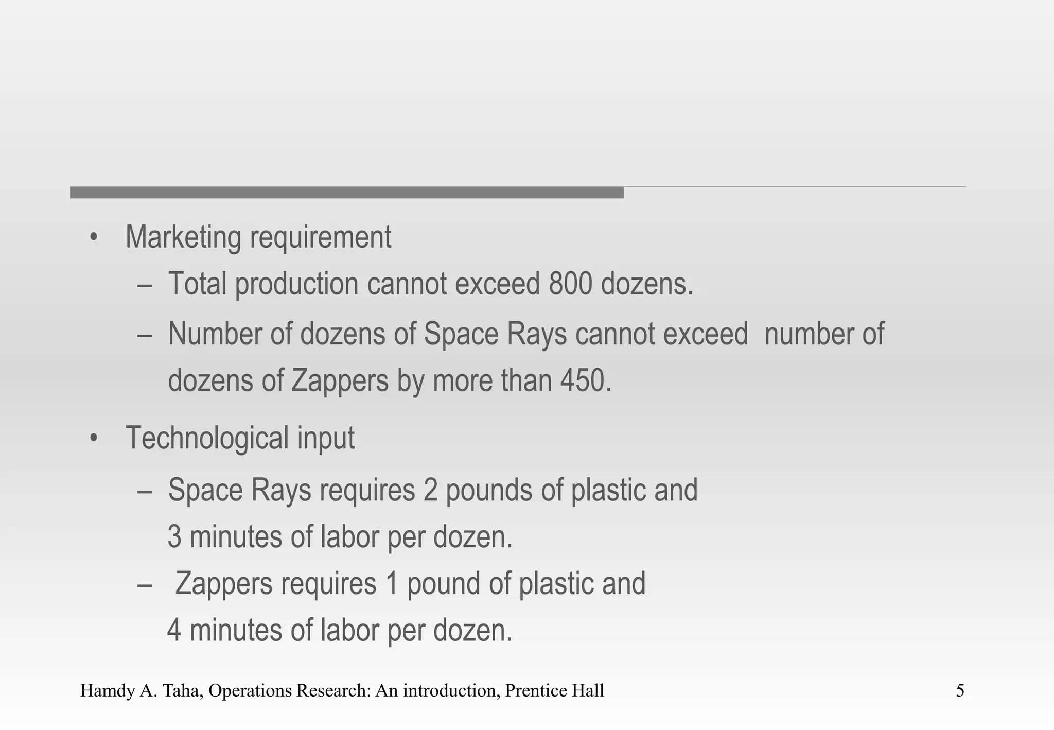
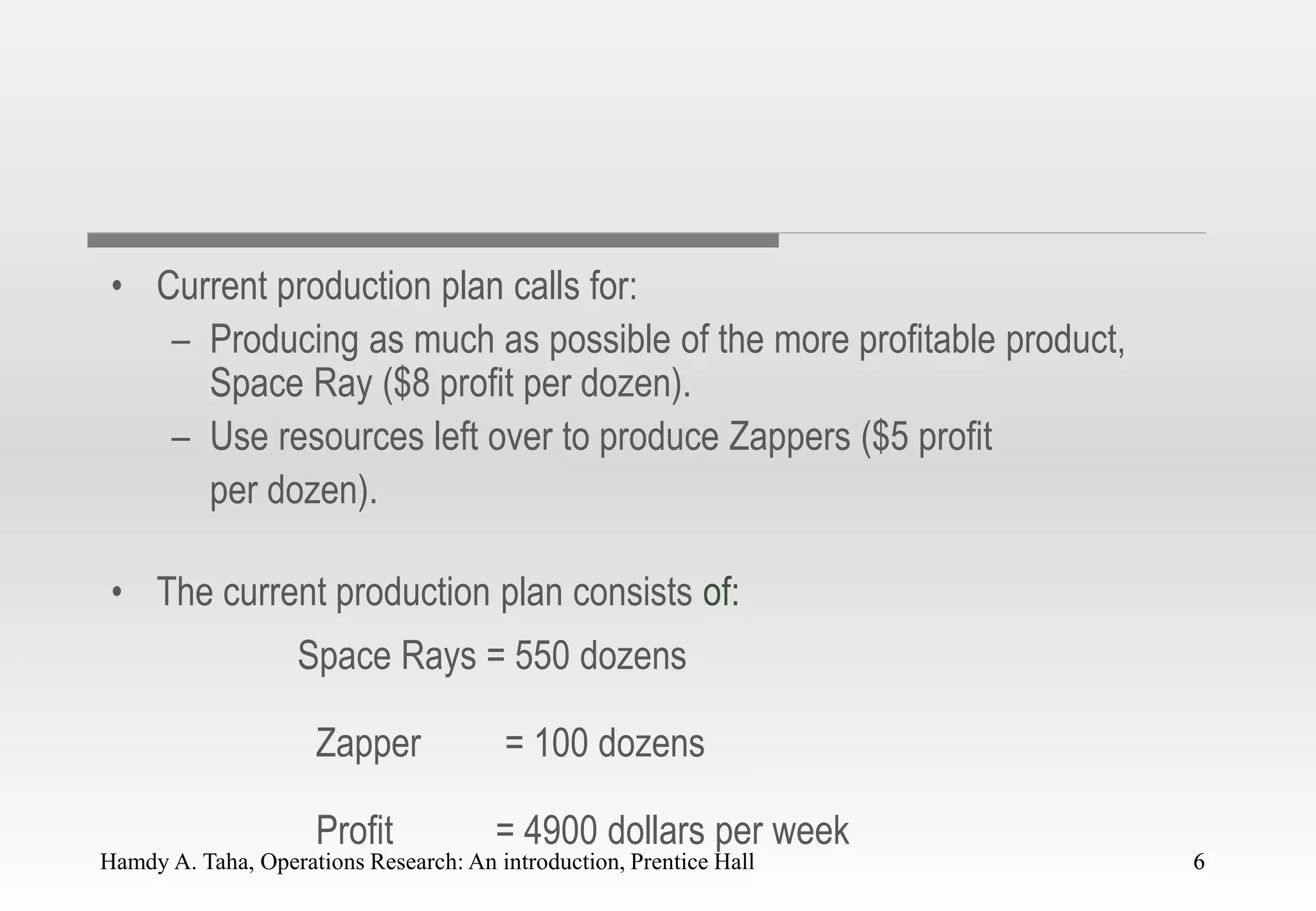
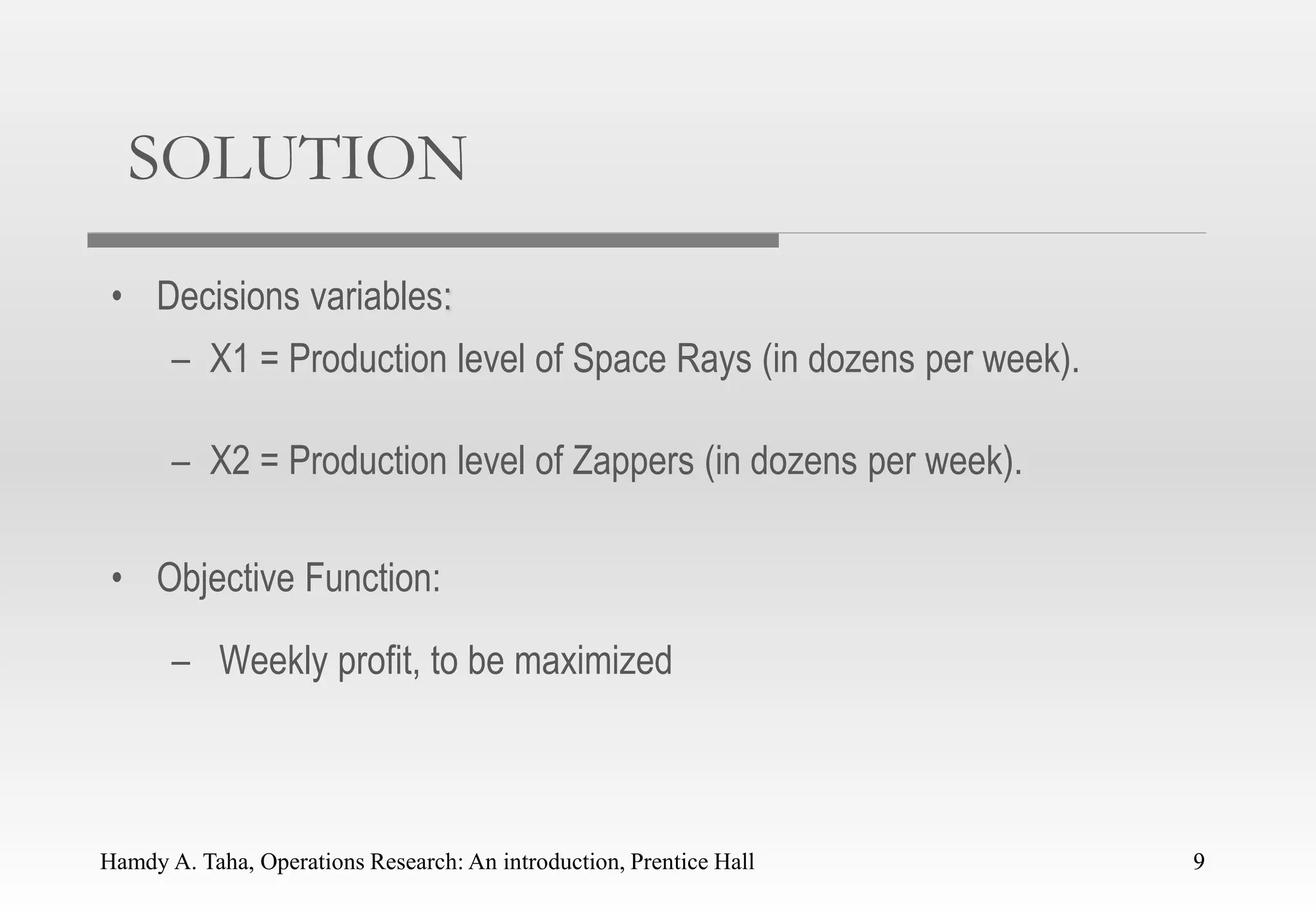
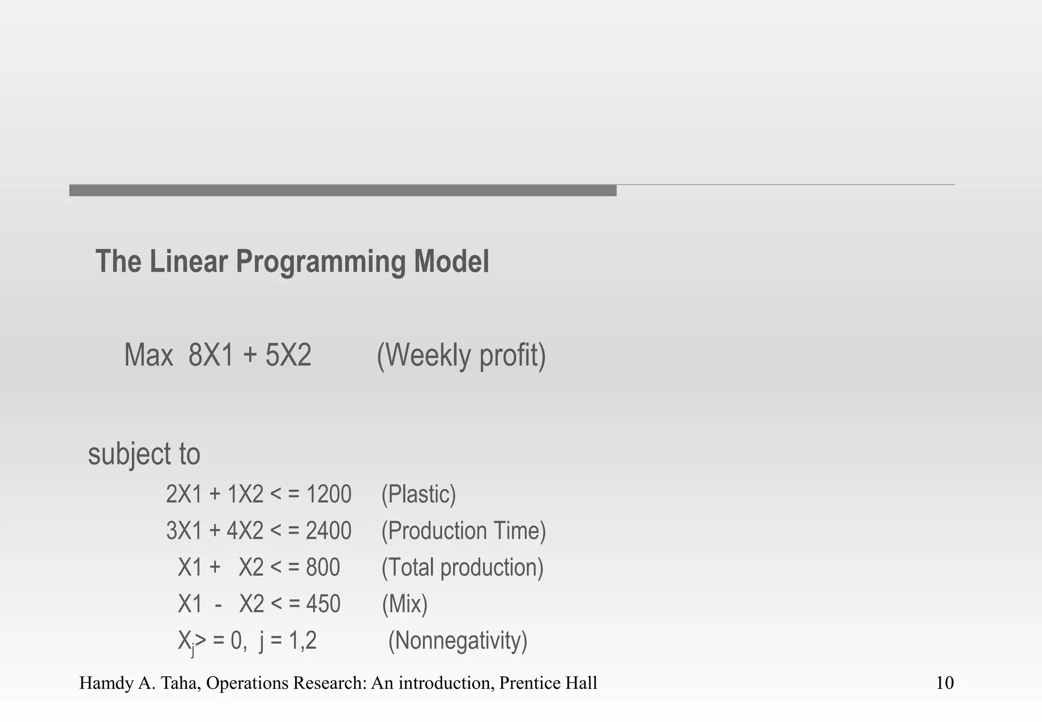
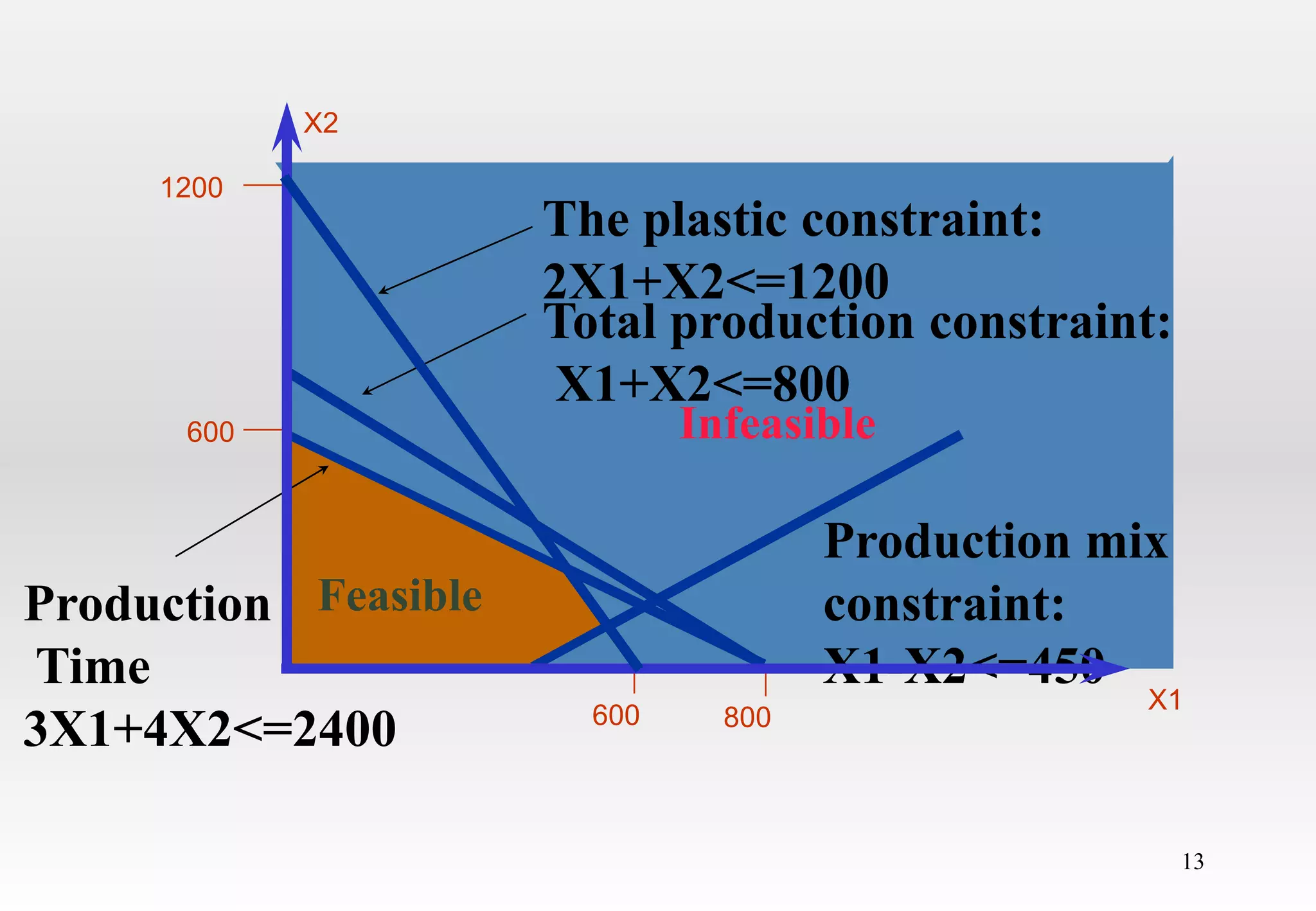
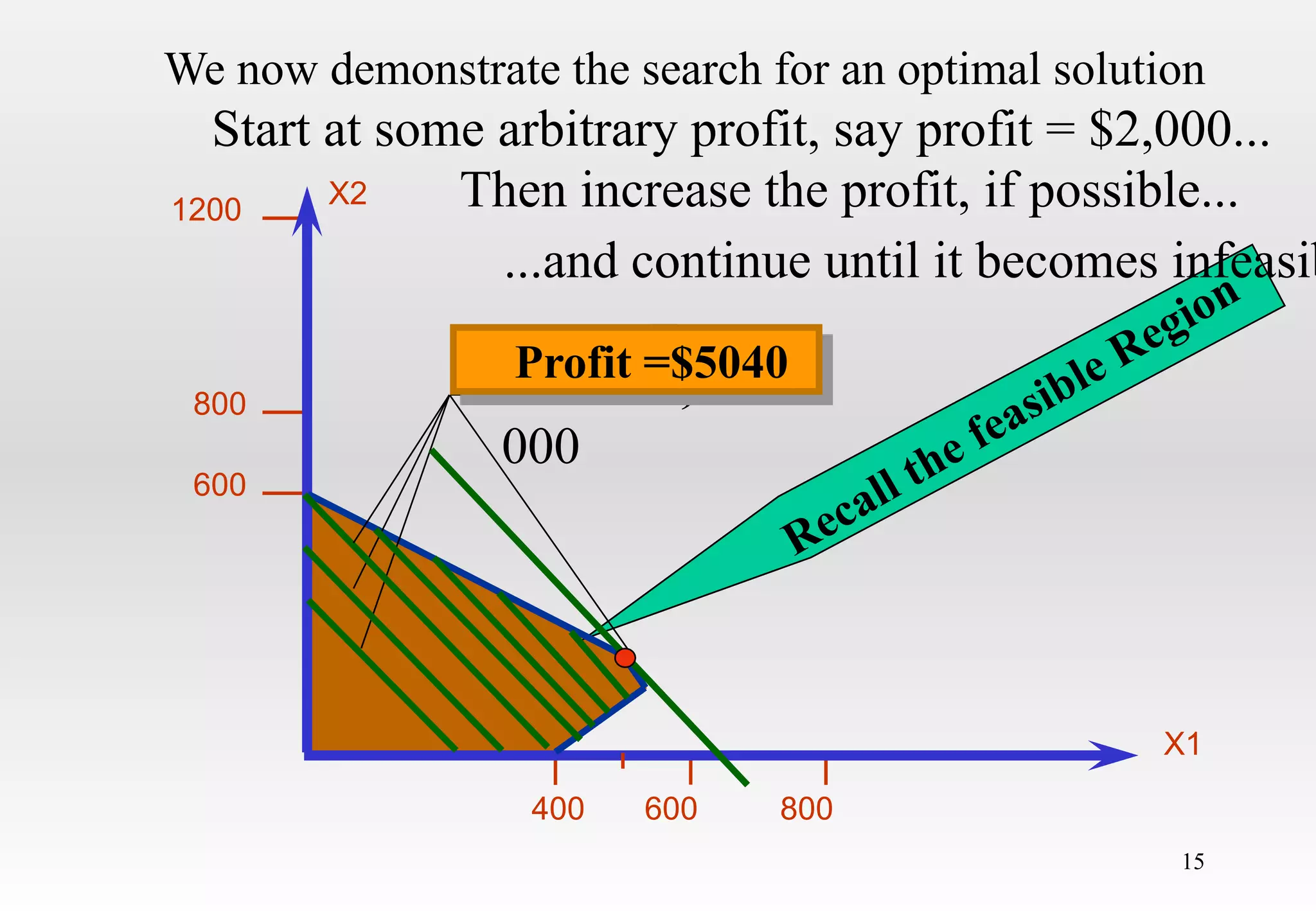
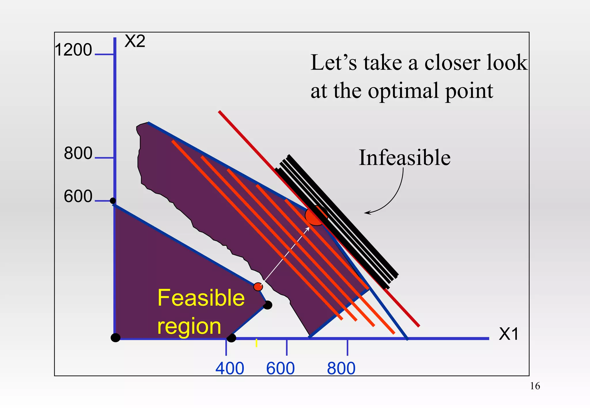
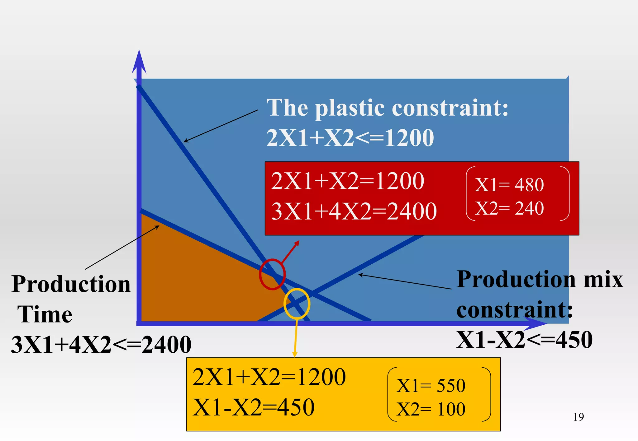
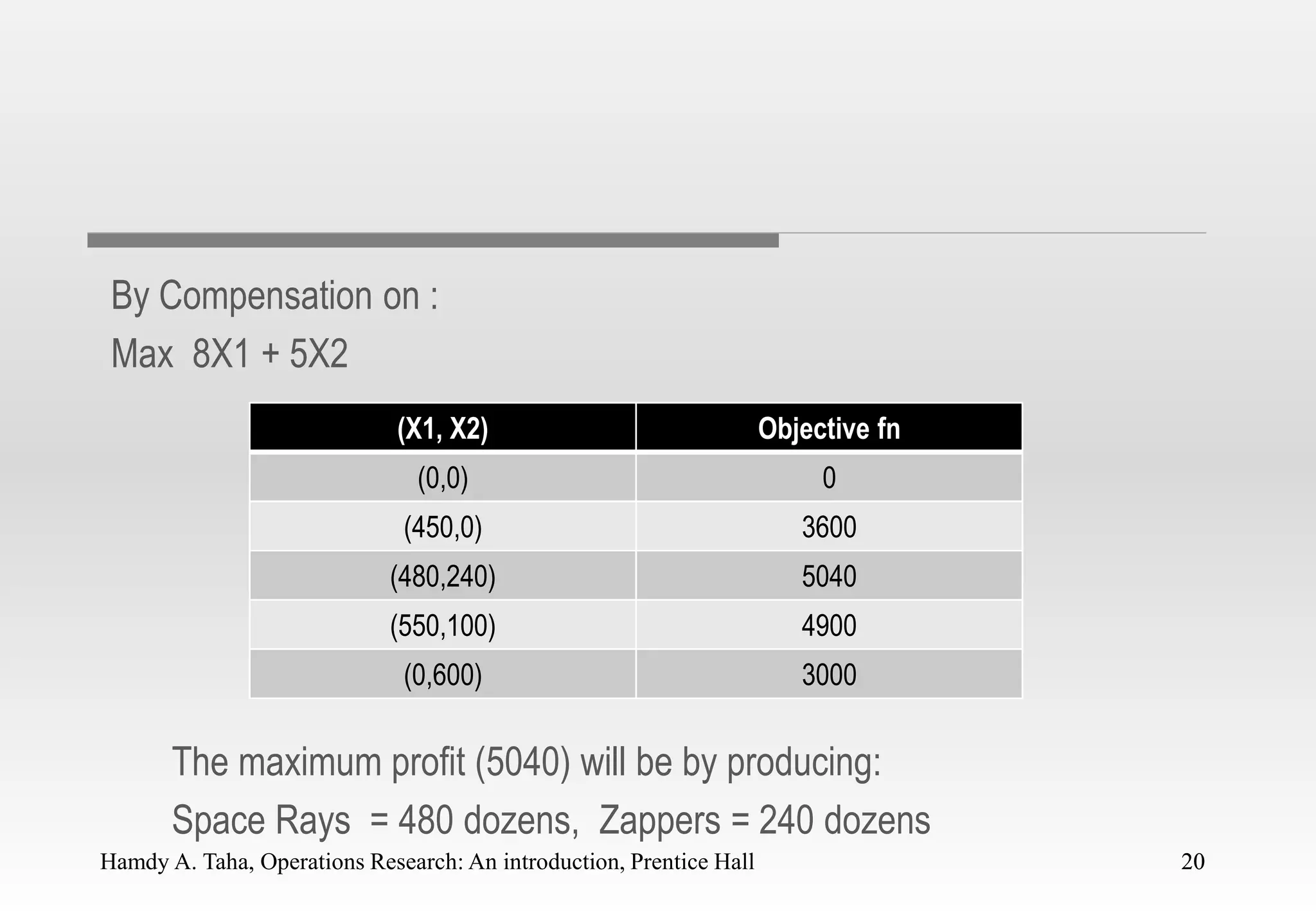
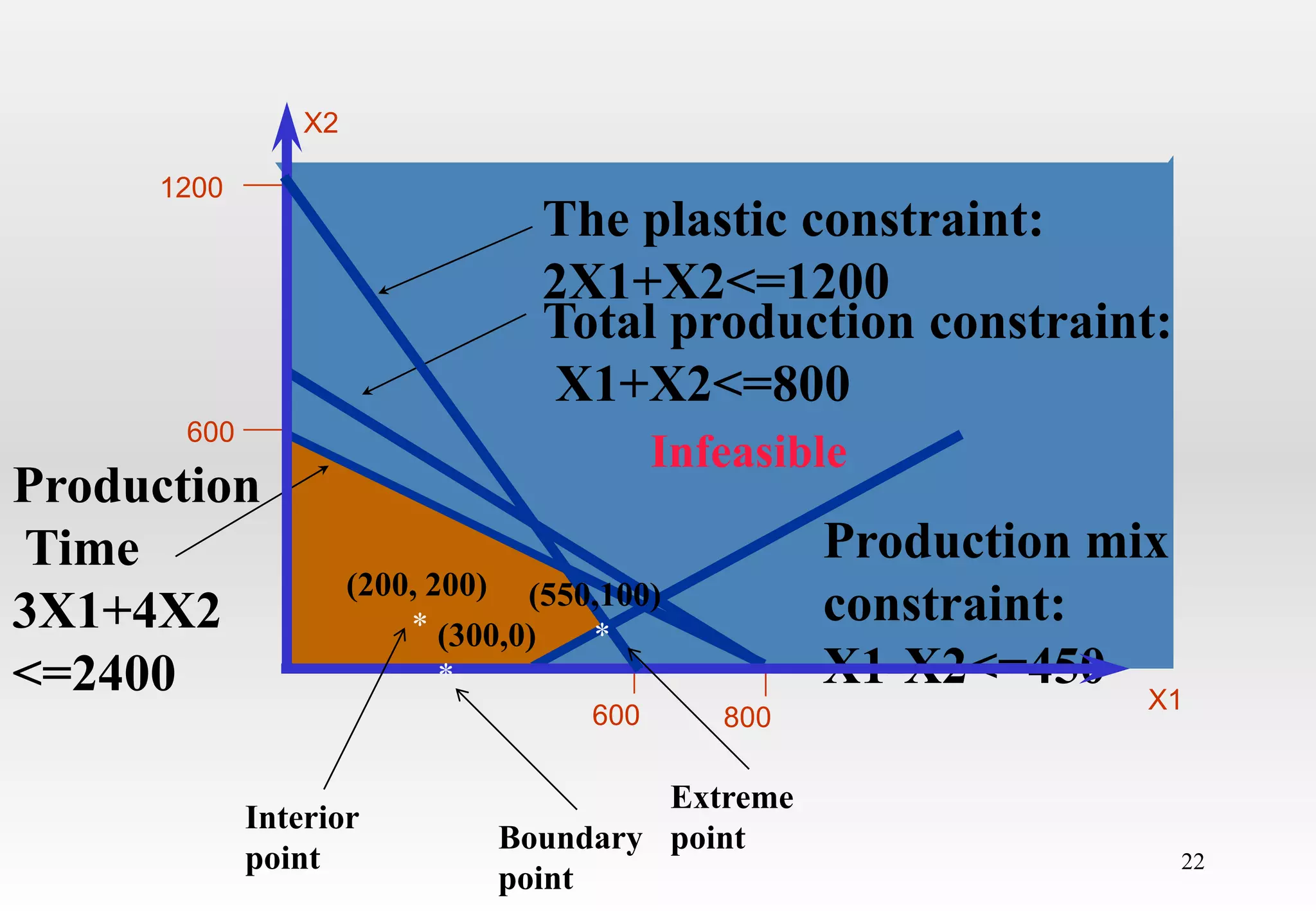
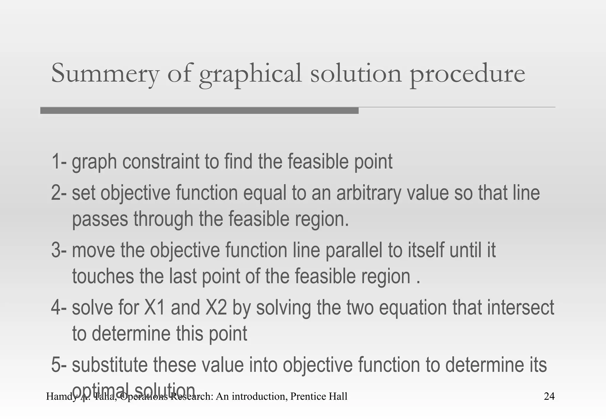
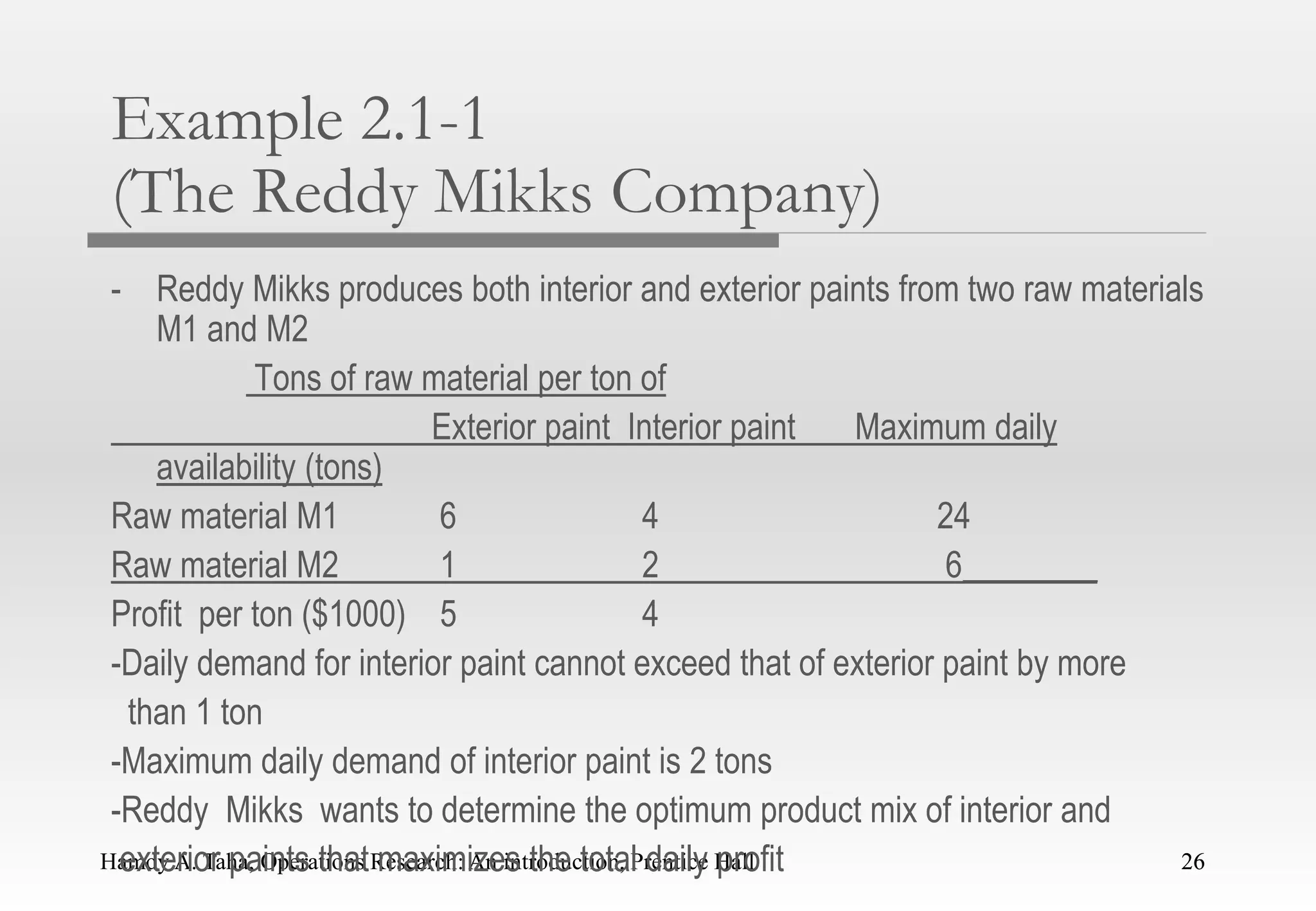
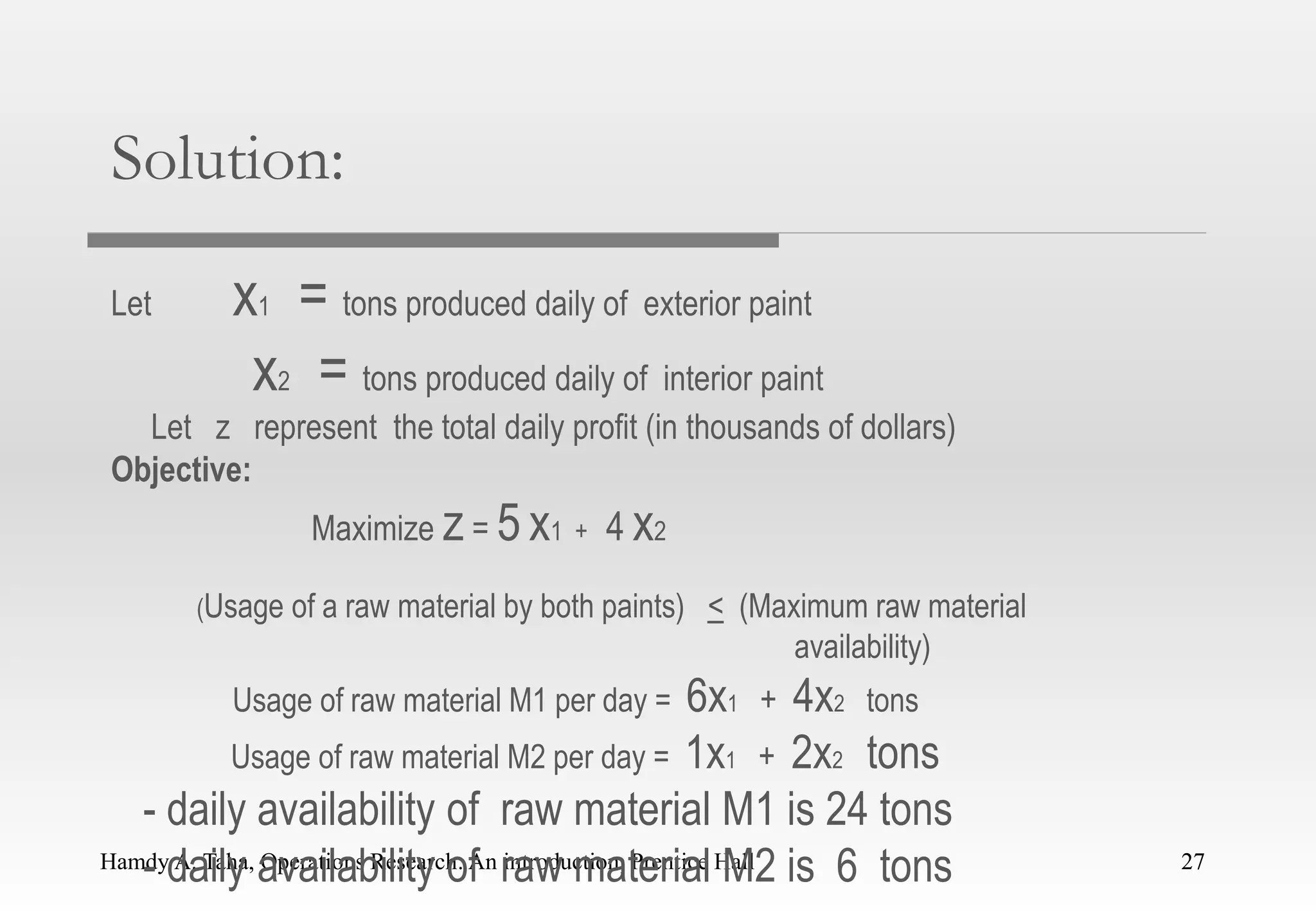
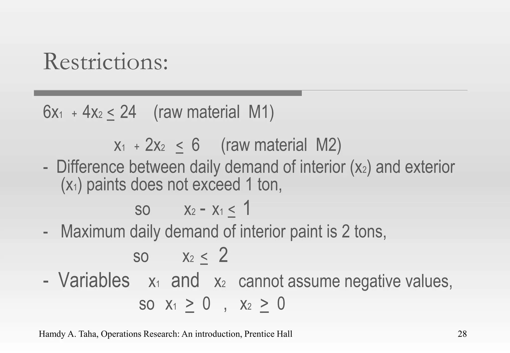
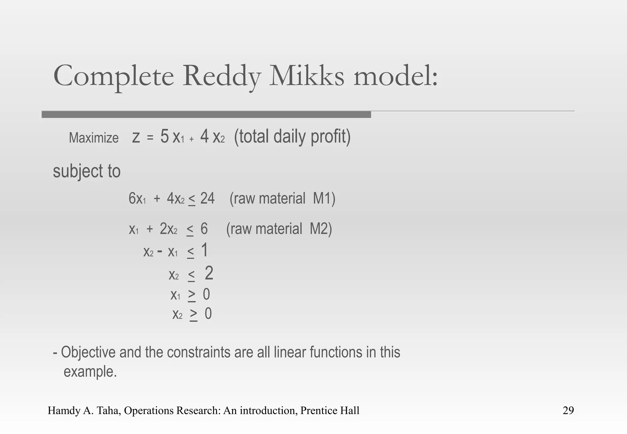
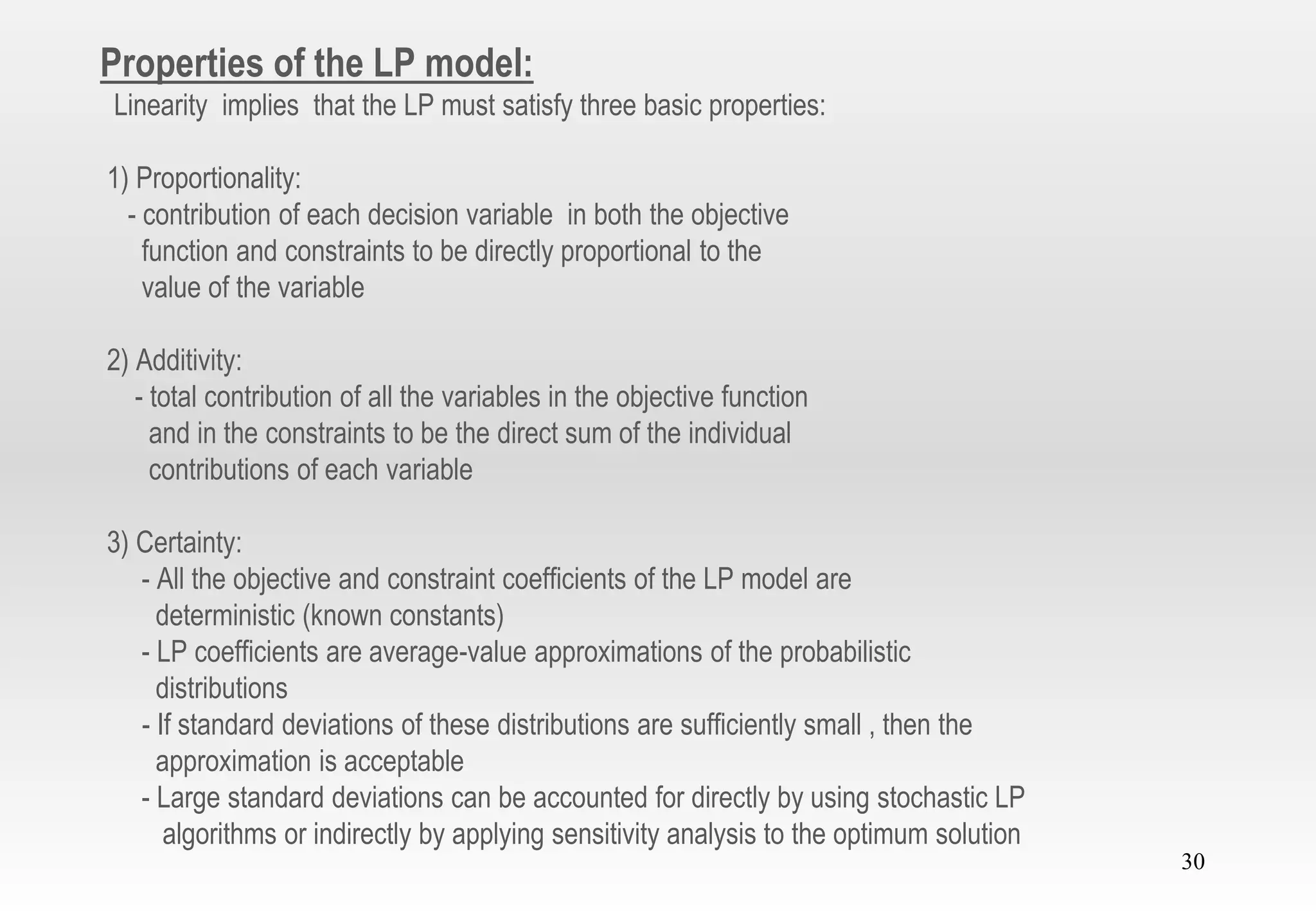
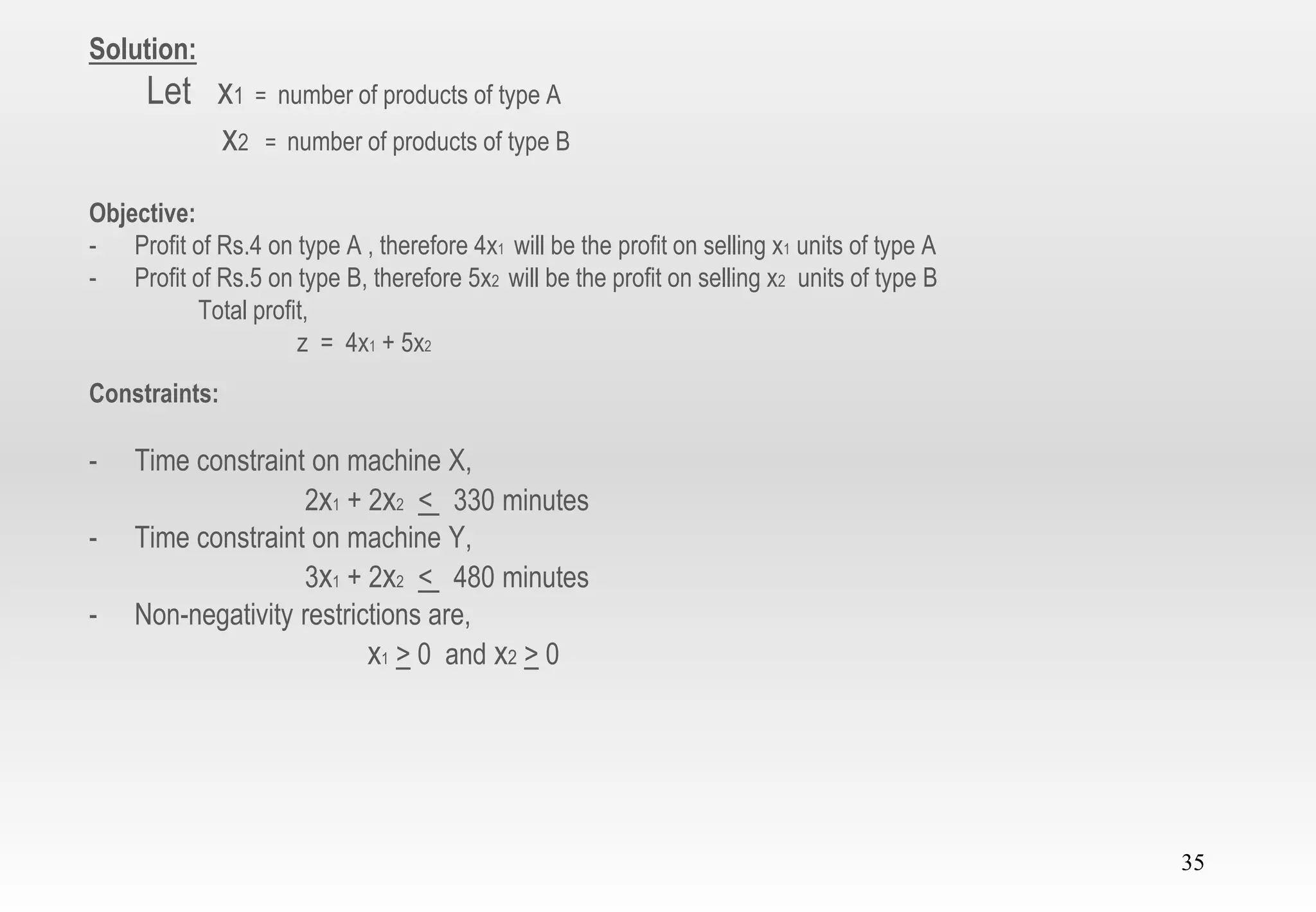
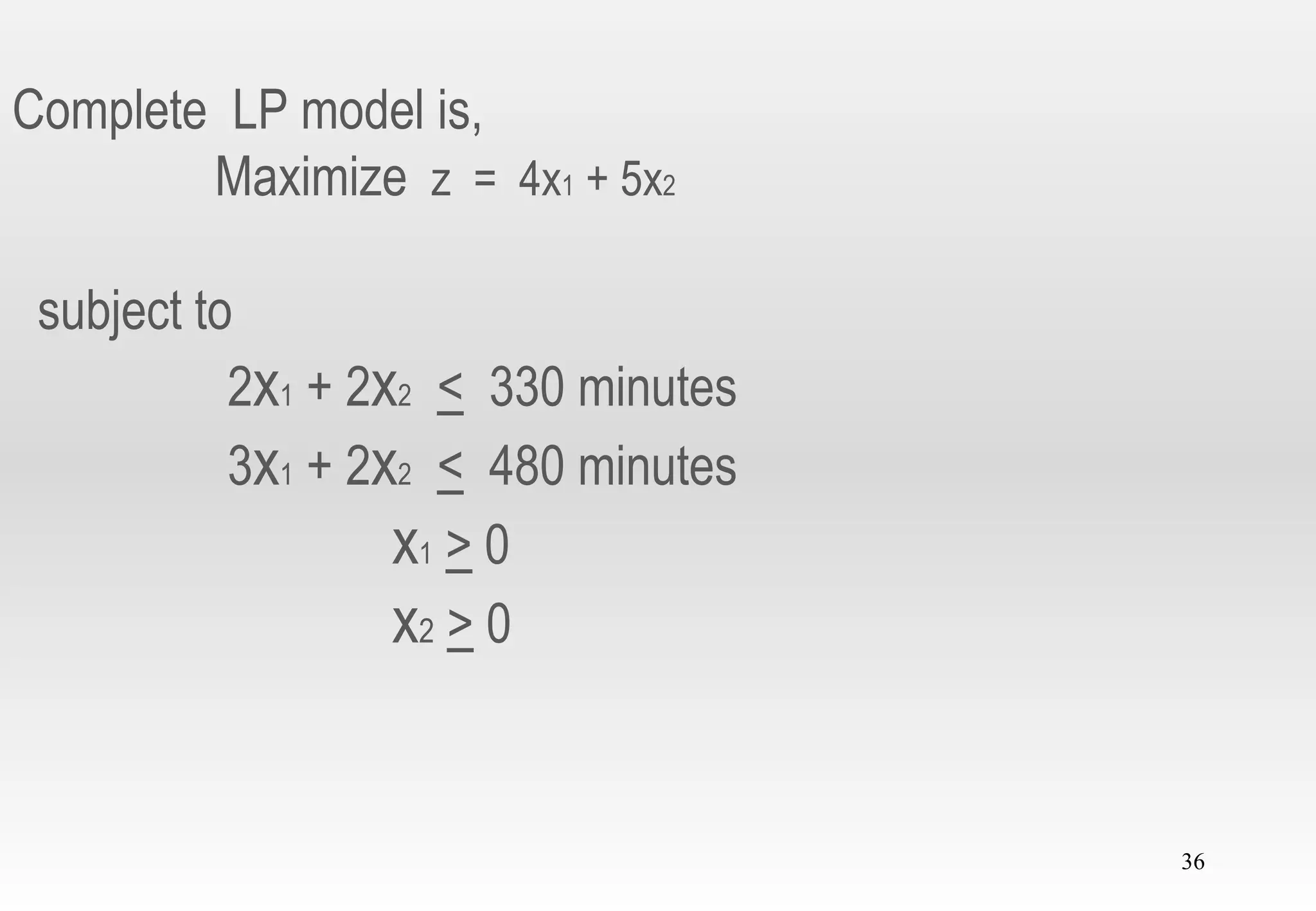
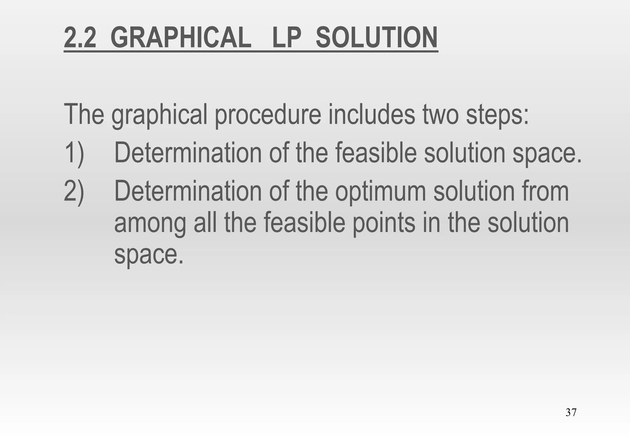
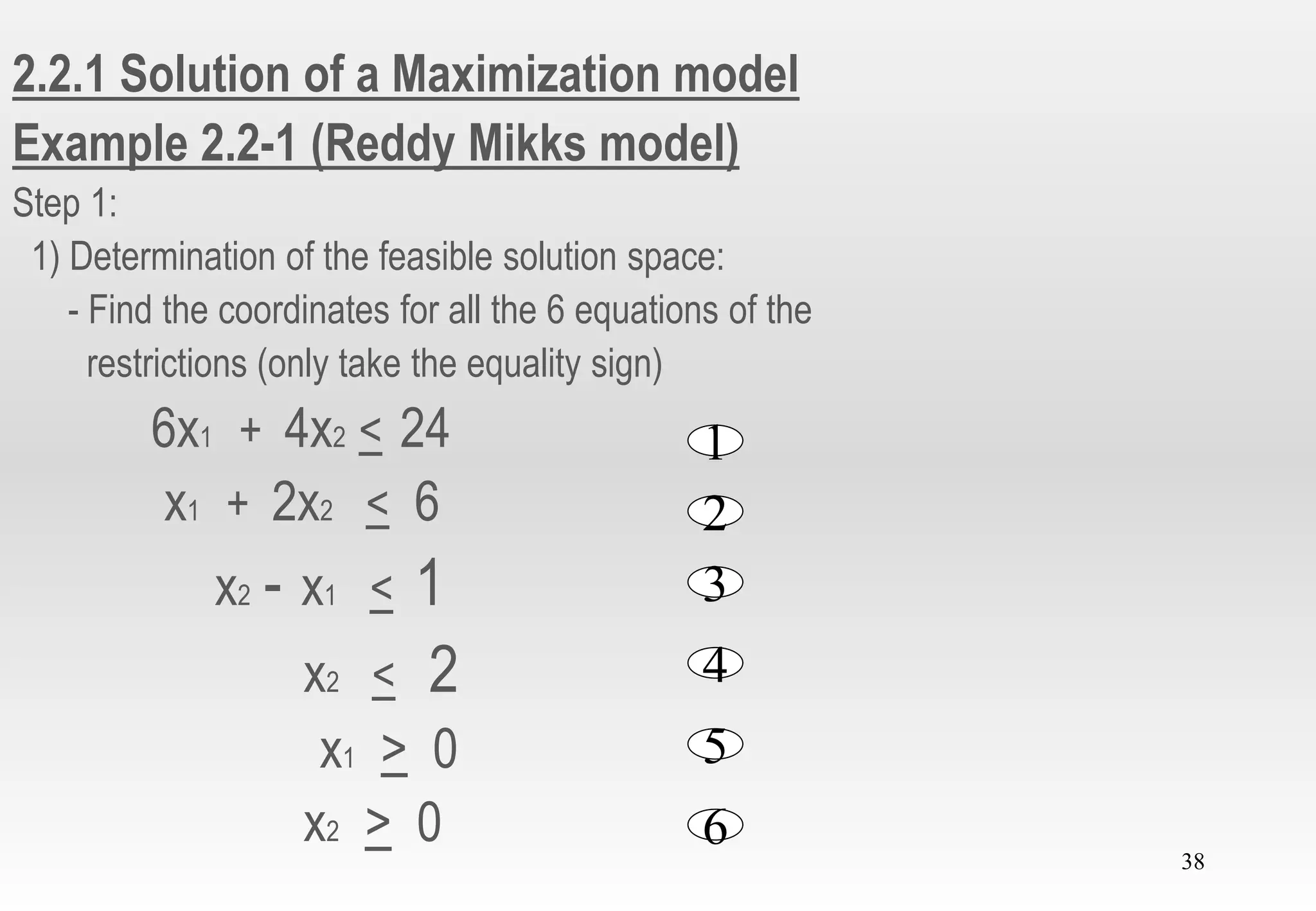
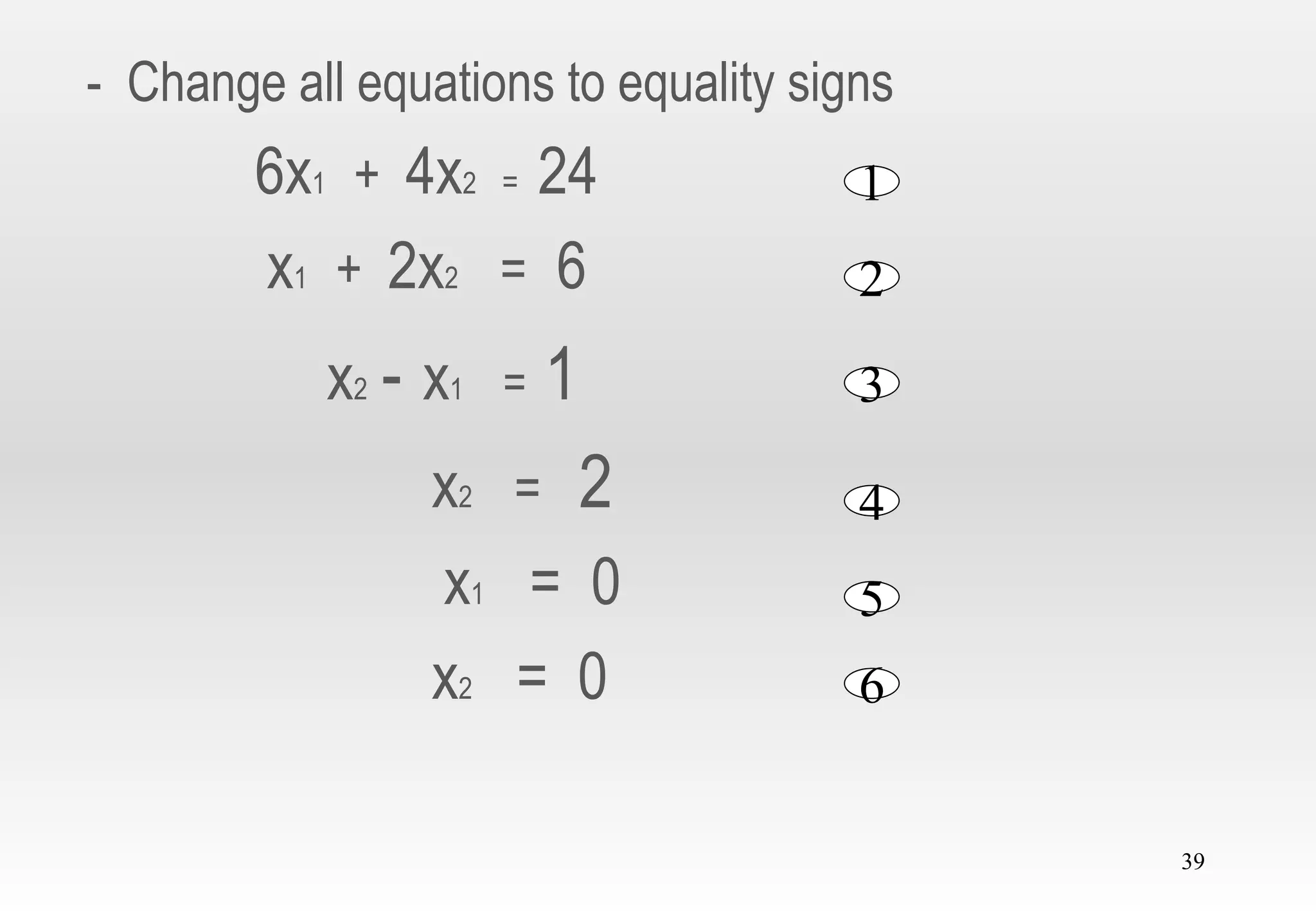
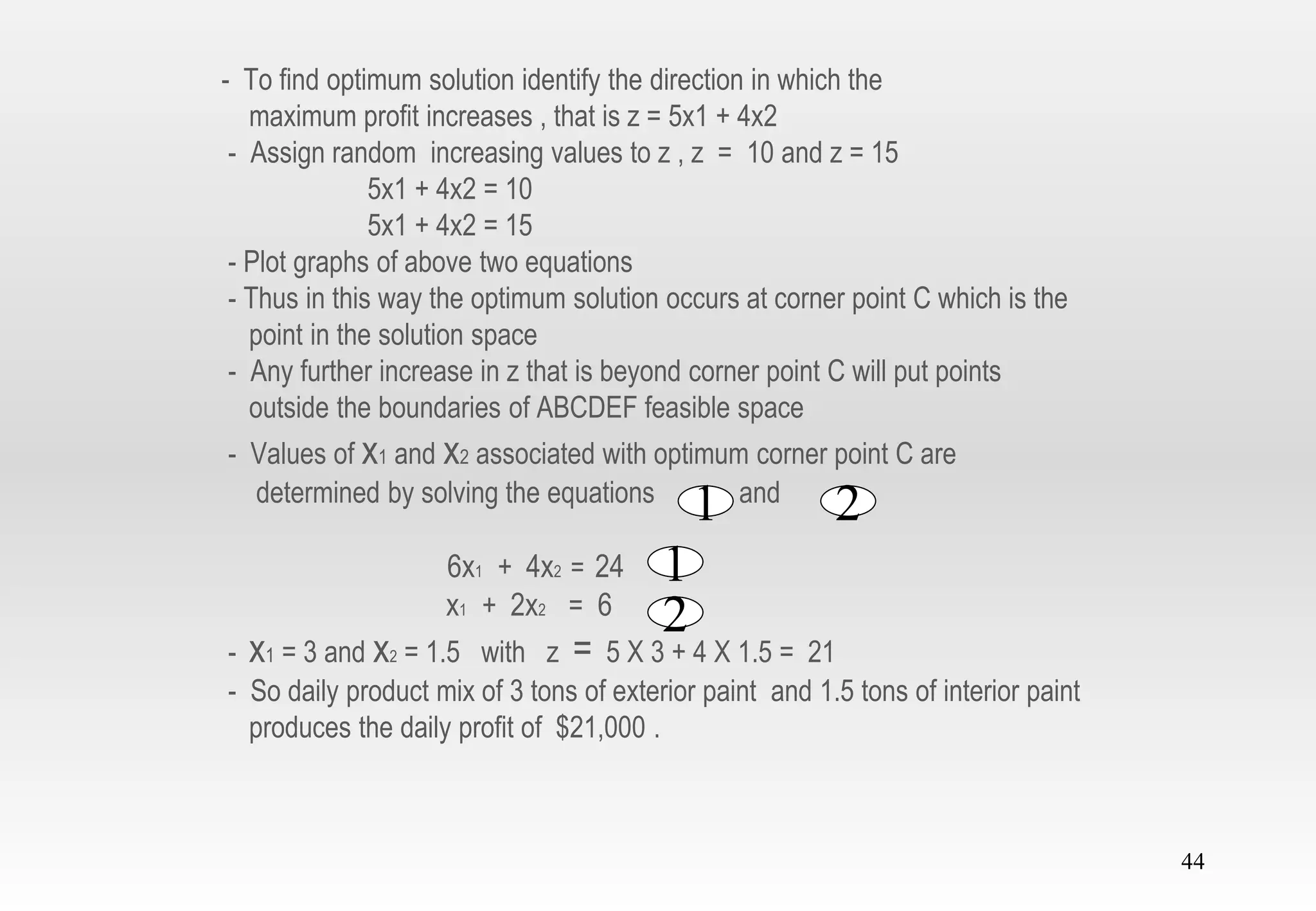
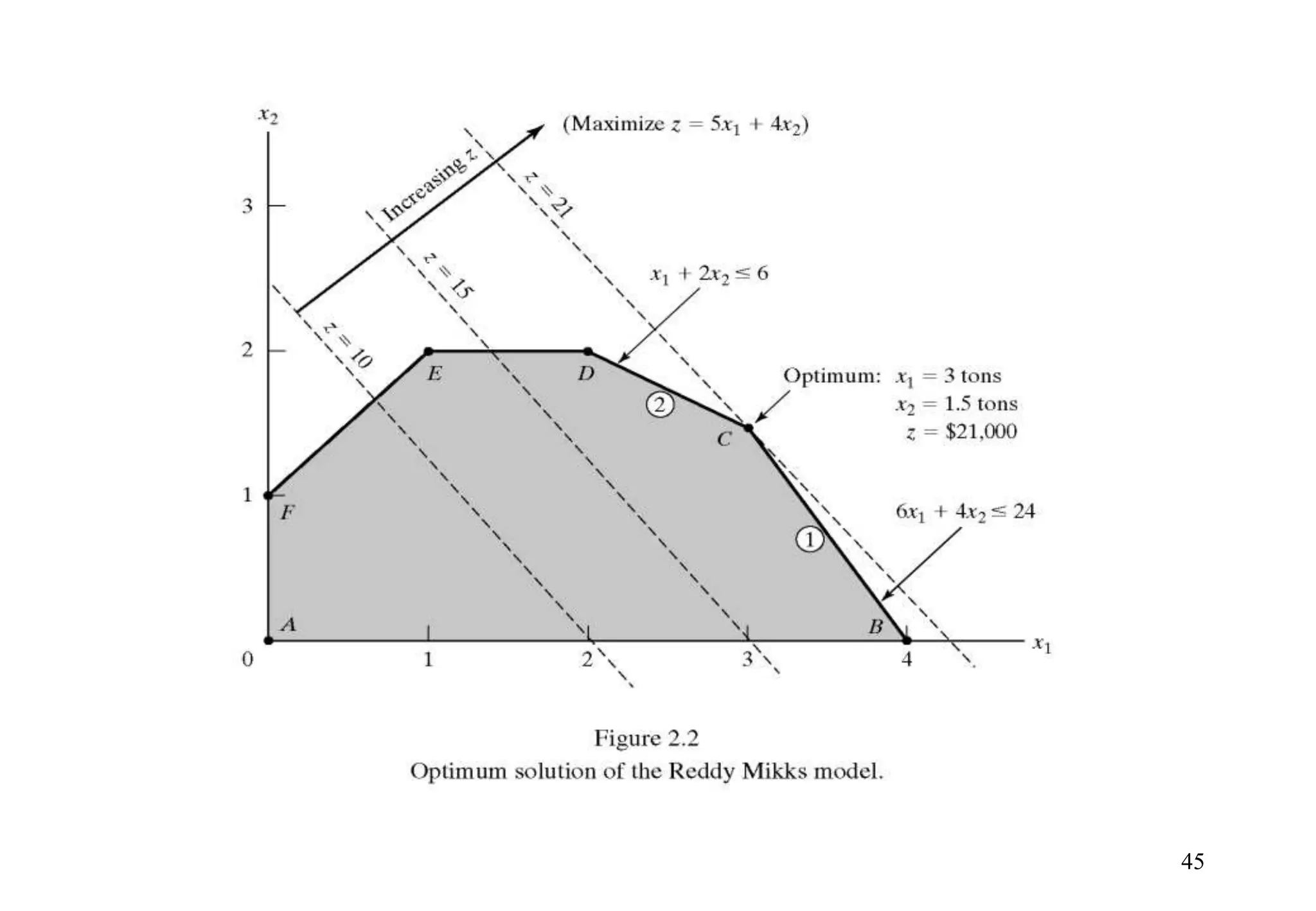
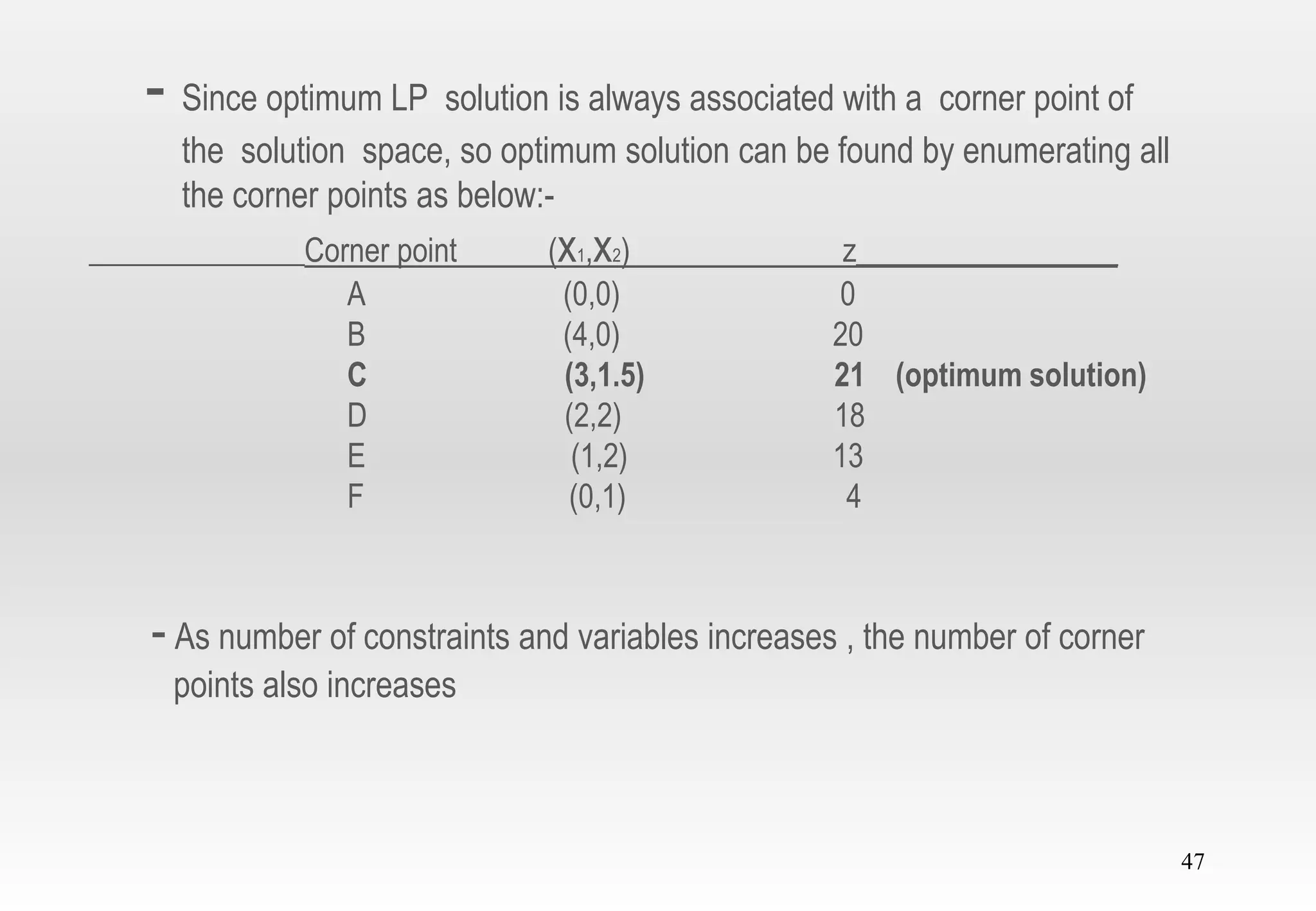
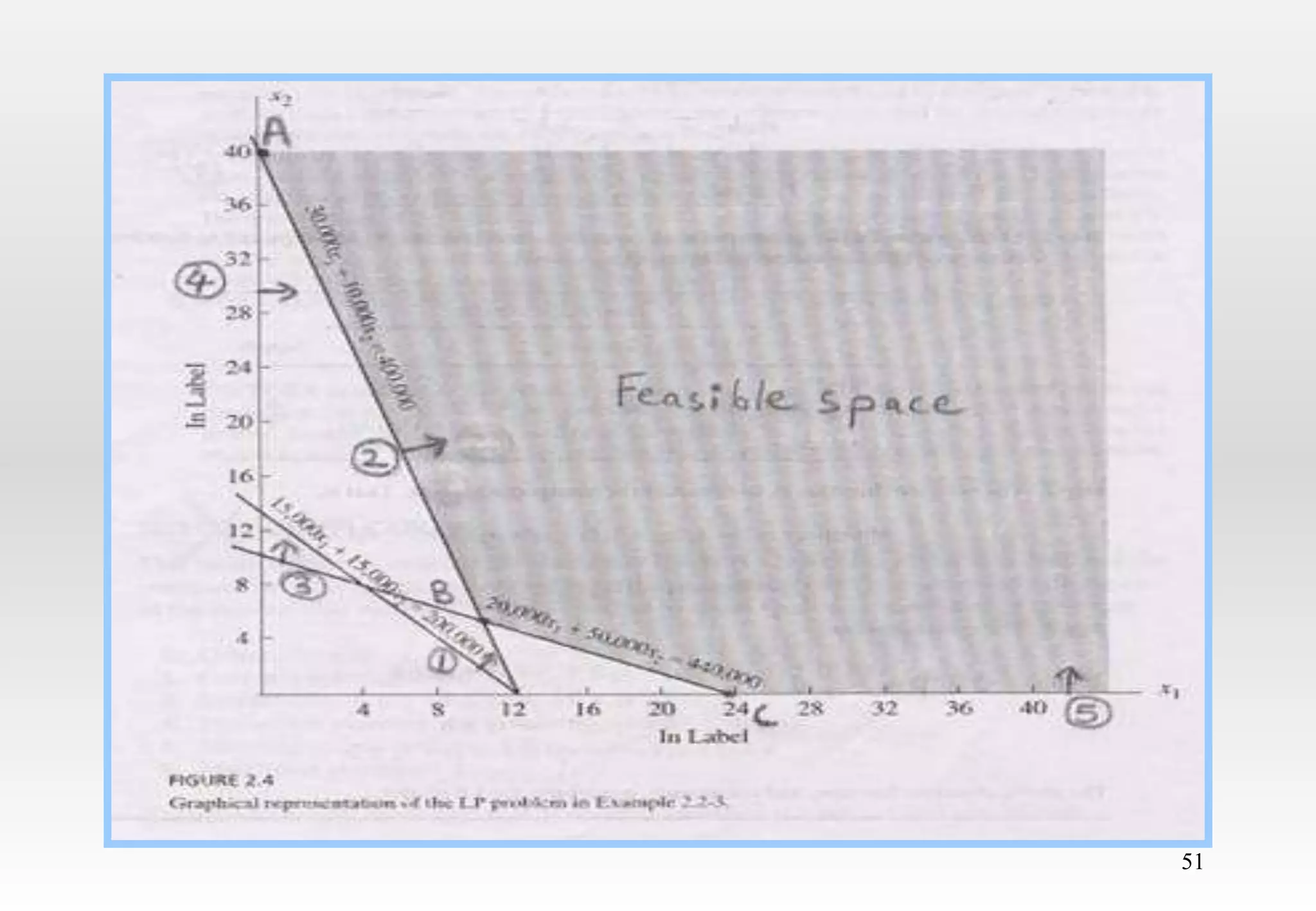
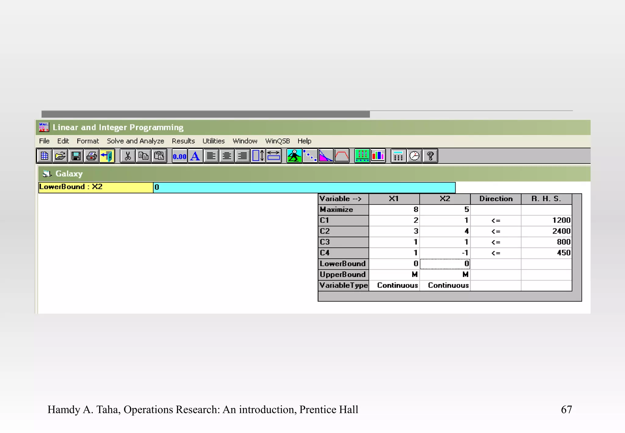
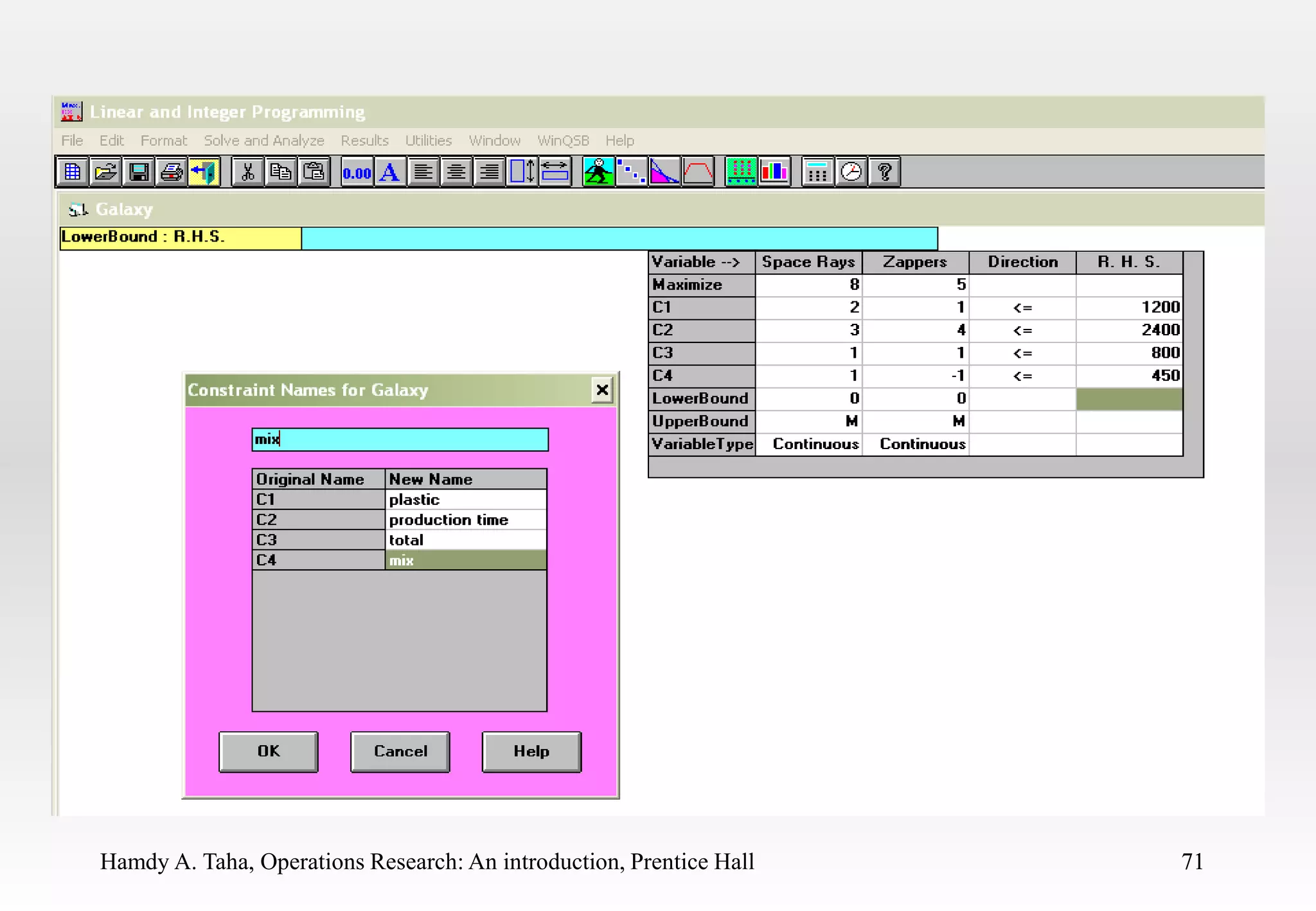
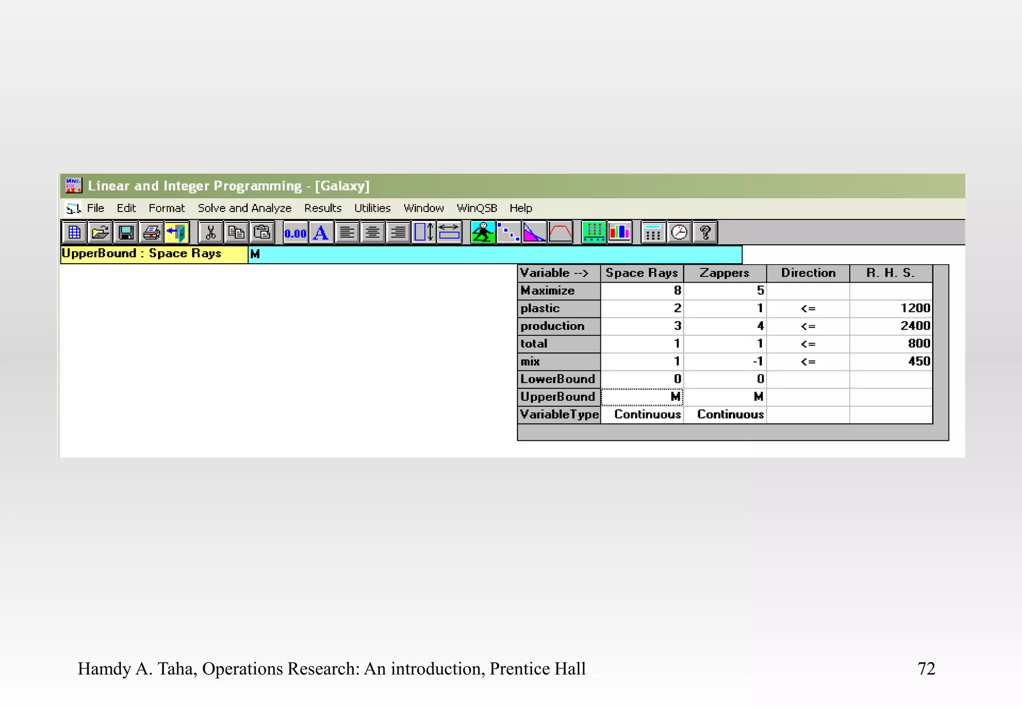
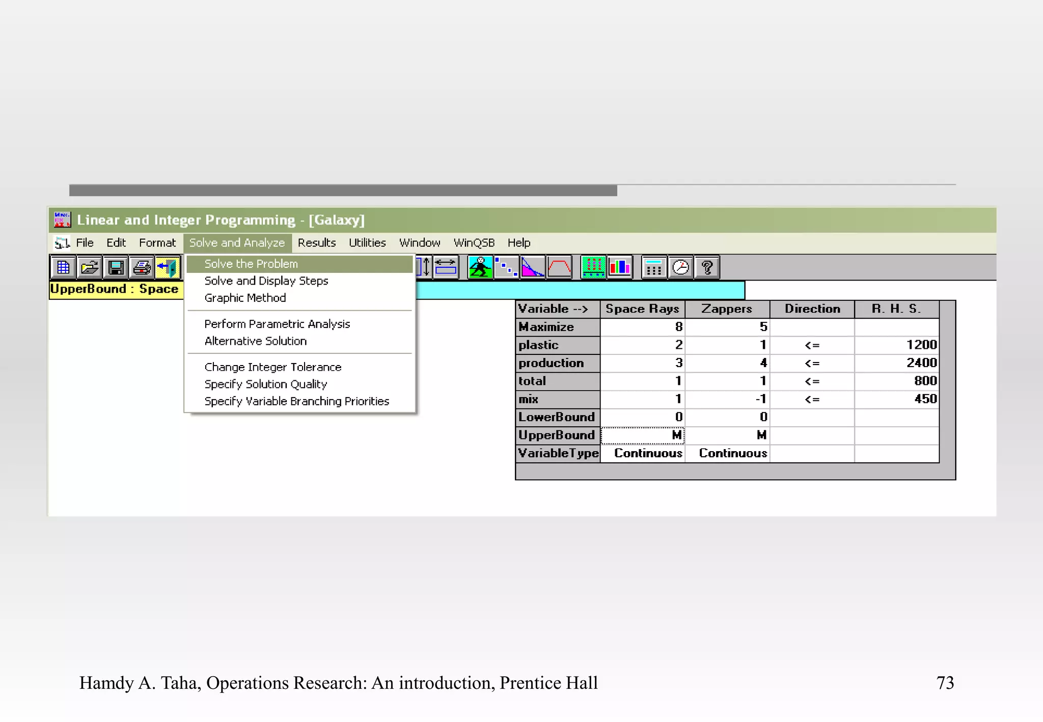
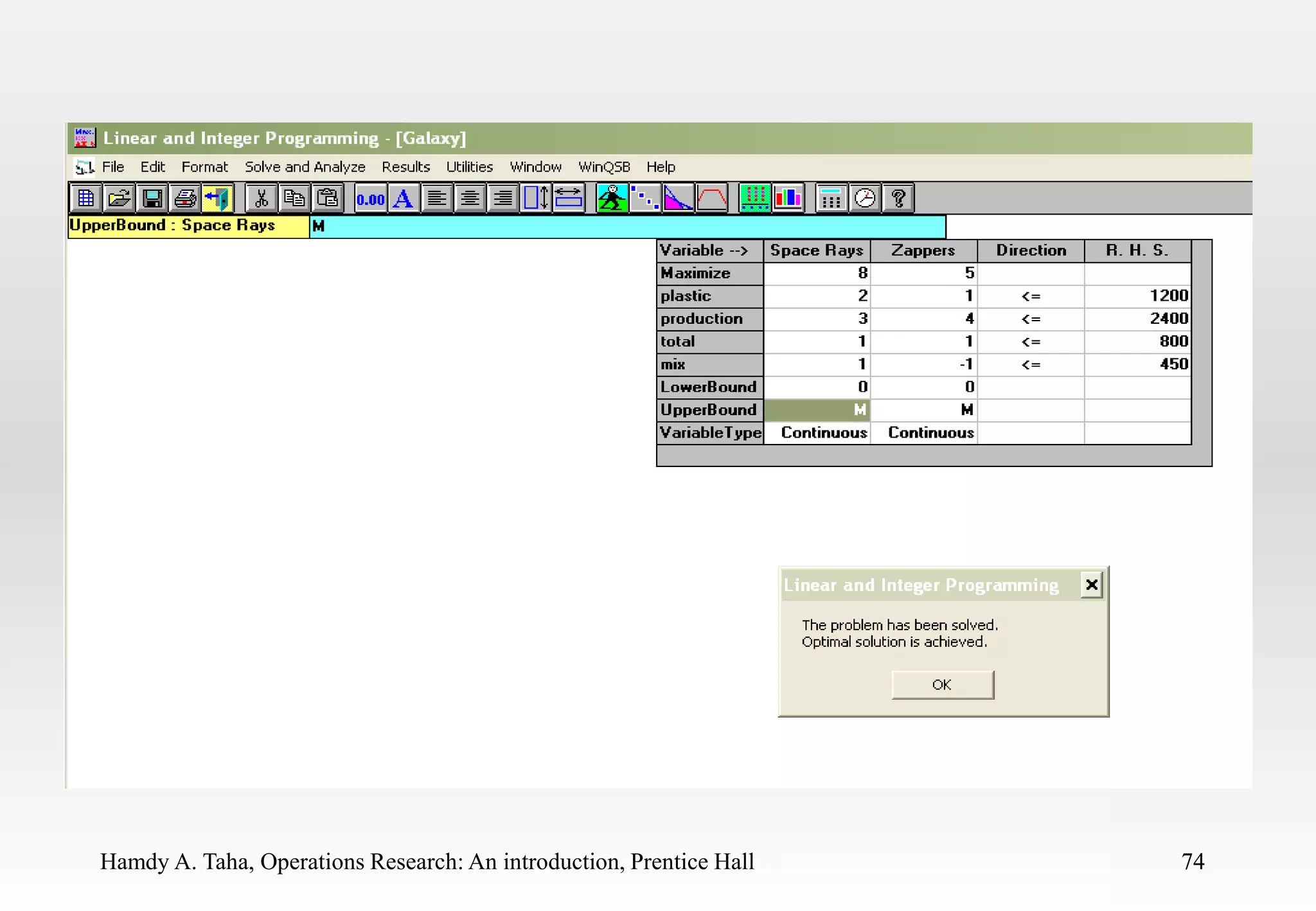
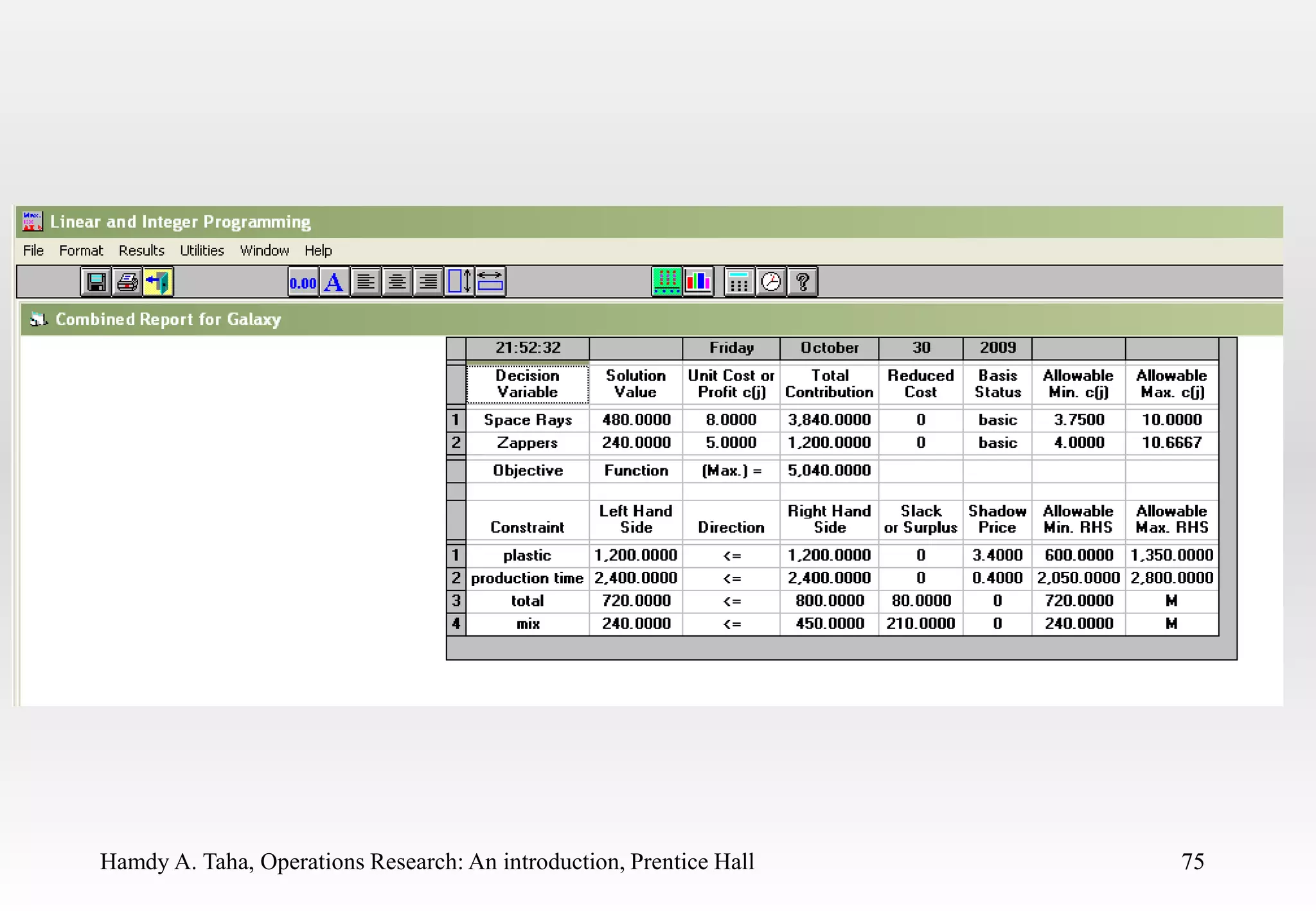
SlideShare a Scribd company logo
1 of 75
Mjdah Al Shehri
Hamdy A. Taha, Operations Research: An
introduction, 8th Edition
Chapter 2:
Modeling with Linear Programming &
sensitivity analysis
1
Hamdy A. Taha, Operations Research: An introduction, Prentice Hall 2
LINEAR PROGRAMMING (LP)
-In mathematics, linear programming (LP) is a technique for
optimization of a linear objective function, subject to linear
equality and linear inequality constraints.
-Linear programming determines the way to achieve the best
outcome (such as maximum profit or lowest cost) in a given
mathematical model and given some list of requirements
represented as linear equations.
2
Hamdy A. Taha, Operations Research: An introduction, Prentice Hall 3
Mathematical formulation of Linear
Programming model:
Step 1
- Study the given situation
- Find the key decision to be made
- Identify the decision variables of the problem
Step 2
- Formulate the objective function to be optimized
Step 3
- Formulate the constraints of the problem
Step 4
- Add non-negativity restrictions or constraints
The objective function , the set of constraints and the non-negativity
restrictions together form an LP model.
3
Hamdy A. Taha, Operations Research: An introduction, Prentice Hall 4
TWO-VARIABLE LP MODEL
EXAMPLE:
“ THE GALAXY INDUSTRY PRODUCTION”
• Galaxy manufactures two toy models:
– Space Ray.
– Zapper.
• Resources are limited to
– 1200 pounds of special plastic.
– 40 hours of production time per week.
4
Hamdy A. Taha, Operations Research: An introduction, Prentice Hall 5
• Marketing requirement
– Total production cannot exceed 800 dozens.
– Number of dozens of Space Rays cannot exceed number of
dozens of Zappers by more than 450.
• Technological input
– Space Rays requires 2 pounds of plastic and
3 minutes of labor per dozen.
– Zappers requires 1 pound of plastic and
4 minutes of labor per dozen.
5
Hamdy A. Taha, Operations Research: An introduction, Prentice Hall 6
• Current production plan calls for:
– Producing as much as possible of the more profitable product,
Space Ray ($8 profit per dozen).
– Use resources left over to produce Zappers ($5 profit
per dozen).
• The current production plan consists of:
Space Rays = 550 dozens
Zapper = 100 dozens
Profit = 4900 dollars per week
6
Management is seeking a
production schedule that will
increase the company’s profit.
7
Hamdy A. Taha, Operations Research: An introduction, Prentice Hall 8
8
A Linear Programming Model
can provide an intelligent
solution to this problem
Hamdy A. Taha, Operations Research: An introduction, Prentice Hall 9
SOLUTION
• Decisions variables:
– X1 = Production level of Space Rays (in dozens per week).
– X2 = Production level of Zappers (in dozens per week).
• Objective Function:
– Weekly profit, to be maximized
9
Hamdy A. Taha, Operations Research: An introduction, Prentice Hall 10
The Linear Programming Model
Max 8X1 + 5X2 (Weekly profit)
subject to
2X1 + 1X2 < = 1200 (Plastic)
3X1 + 4X2 < = 2400 (Production Time)
X1 + X2 < = 800 (Total production)
X1 - X2 < = 450 (Mix)
Xj> = 0, j = 1,2 (Nonnegativity)
10
Hamdy A. Taha, Operations Research: An introduction, Prentice Hall 11
Feasible Solutions for Linear
Programs
• The set of all points that satisfy all the constraints of the model is
called
11
FEASIBLE REGION
Hamdy A. Taha, Operations Research: An introduction, Prentice Hall 12
Using a graphical presentation we can represent all the constraints,
the objective function, and the three types of feasible points.
12
13
1200
600
The Plastic constraint
Feasible
The plastic constraint:
2X1+X2<=1200
X2
Infeasible
Production
Time
3X1+4X2<=2400
Total production constraint:
X1+X2<=800
600
800
Production mix
constraint:
X1-X2<=450
X1
14
Solving Graphically for an
Optimal Solution
15
600
800
1200
400 600 800
X2
X1
We now demonstrate the search for an optimal solution
Start at some arbitrary profit, say profit = $2,000...
Profit = $
000
2,
Then increase the profit, if possible...
3,
4,
...and continue until it becomes infeasib
Profit =$5040
16
600
800
1200
400 600 800
X2
X1
Let’s take a closer look
at the optimal point
Feasible
region
Feasible
region
Infeasible
17
1200
600
The Plastic constraint
Feasible
The plastic constraint:
2X1+X2<=1200
X2
Infeasible
Production
Time
3X1+4X2<=2400
Total production constraint:
X1+X2<=800
600
800
Production mix
constraint:
X1-X2<=450
X1
A (0,600)
E (0,0)
B (480,240)
C (550,100)
D (450,0)
Hamdy A. Taha, Operations Research: An introduction, Prentice Hall 18
• To determine the value for X1 and X2 at the optimal
point, the two equations of the binding constraint
must be solved.
18
Production mix
constraint:
X1-X2<=450
19
The plastic constraint:
2X1+X2<=1200
Production
Time
3X1+4X2<=2400
2X1+X2=1200
3X1+4X2=2400
X1= 480
X2= 240
2X1+X2=1200
X1-X2=450
X1= 550
X2= 100
Hamdy A. Taha, Operations Research: An introduction, Prentice Hall 20
By Compensation on :
Max 8X1 + 5X2
The maximum profit (5040) will be by producing:
Space Rays = 480 dozens, Zappers = 240 dozens
20
(X1, X2) Objective fn
(0,0) 0
(450,0) 3600
(480,240) 5040
(550,100) 4900
(0,600) 3000
Hamdy A. Taha, Operations Research: An introduction, Prentice Hall 21
Type of feasible points
• Interior point: satisfies all constraint but non with
equality.
• Boundary points: satisfies all constraints, at least one
with equality
• Extreme point: satisfies all constraints, two with
equality.
21
22
1200
600
The Plastic constraint
The plastic constraint:
2X1+X2<=1200
X2
Infeasible
Production
Time
3X1+4X2
<=2400
Total production constraint:
X1+X2<=800
600
800
Production mix
constraint:
X1-X2<=450
X1
(200, 200)
*
Interior
point
(300,0)
*
Boundary
point
(550,100)
*
Extreme
point
Hamdy A. Taha, Operations Research: An introduction, Prentice Hall 23
• If a linear programming has an optimal solution , an
extreme point is optimal.
23
Hamdy A. Taha, Operations Research: An introduction, Prentice Hall 24
Summery of graphical solution procedure
1- graph constraint to find the feasible point
2- set objective function equal to an arbitrary value so that line
passes through the feasible region.
3- move the objective function line parallel to itself until it
touches the last point of the feasible region .
4- solve for X1 and X2 by solving the two equation that intersect
to determine this point
5- substitute these value into objective function to determine its
optimal solution. 24
Hamdy A. Taha, Operations Research: An introduction, Prentice Hall 25
MORE EXAMPLE
25
Hamdy A. Taha, Operations Research: An introduction, Prentice Hall 26
Example 2.1-1
(The Reddy Mikks Company)
- Reddy Mikks produces both interior and exterior paints from two raw materials
M1 and M2
Tons of raw material per ton of
Exterior paint Interior paint Maximum daily
availability (tons)
Raw material M1 6 4 24
Raw material M2 1 2 6________
Profit per ton ($1000) 5 4
-Daily demand for interior paint cannot exceed that of exterior paint by more
than 1 ton
-Maximum daily demand of interior paint is 2 tons
-Reddy Mikks wants to determine the optimum product mix of interior and
exterior paints that maximizes the total daily profit 26
Hamdy A. Taha, Operations Research: An introduction, Prentice Hall 27
Solution:
Let x1 = tons produced daily of exterior paint
x2 = tons produced daily of interior paint
Let z represent the total daily profit (in thousands of dollars)
Objective:
Maximize z = 5 x1 + 4 x2
(Usage of a raw material by both paints) < (Maximum raw material
availability)
Usage of raw material M1 per day = 6x1 + 4x2 tons
Usage of raw material M2 per day = 1x1 + 2x2 tons
- daily availability of raw material M1 is 24 tons
- daily availability of raw material M2 is 6 tons 27
Hamdy A. Taha, Operations Research: An introduction, Prentice Hall 28
Restrictions:
6x1 + 4x2 < 24 (raw material M1)
x1 + 2x2 < 6 (raw material M2)
- Difference between daily demand of interior (x2) and exterior
(x1) paints does not exceed 1 ton,
so x2 - x1 < 1
- Maximum daily demand of interior paint is 2 tons,
so x2 < 2
- Variables x1 and x2 cannot assume negative values,
so x1 > 0 , x2 > 0
28
Hamdy A. Taha, Operations Research: An introduction, Prentice Hall 29
Complete Reddy Mikks model:
Maximize z = 5 x1 + 4 x2 (total daily profit)
subject to
6x1 + 4x2 < 24 (raw material M1)
x1 + 2x2 < 6 (raw material M2)
x2 - x1 < 1
x2 < 2
x1 > 0
x2 > 0
- Objective and the constraints are all linear functions in this
example.
29
30
Properties of the LP model:
Linearity implies that the LP must satisfy three basic properties:
1) Proportionality:
- contribution of each decision variable in both the objective
function and constraints to be directly proportional to the
value of the variable
2) Additivity:
- total contribution of all the variables in the objective function
and in the constraints to be the direct sum of the individual
contributions of each variable
3) Certainty:
- All the objective and constraint coefficients of the LP model are
deterministic (known constants)
- LP coefficients are average-value approximations of the probabilistic
distributions
- If standard deviations of these distributions are sufficiently small , then the
approximation is acceptable
- Large standard deviations can be accounted for directly by using stochastic LP
algorithms or indirectly by applying sensitivity analysis to the optimum solution
Hamdy A. Taha, Operations Research: An introduction, Prentice Hall 31
Example 2.1-2
(Problem Mix Model)
- Two machines X and Y
- X is designed for 5-ounce bottles
- Y is designed for 10-ounce bottles
- X can also produce 10-ounce bottles with some loss of
efficiency
- Y can also produce 5-ounce bottles with some loss of
efficiency
31
32
Machine 5-ounce bottles 10-ounce bottles
X 80/min 30/min
Y 40/min 50/min
- X and Y machines can run 8 hours per day for 5 days a
week
- Profit on 5-ounce bottle is 20 paise
- Profit on 10-ounce bottle is 30 paise
- Weekly production of the drink cannot exceed 500,000
ounces
- Market can utilize 30,000 (5-ounce) bottles and 8000 (10-
ounce) bottles per week
- To maximize the profit
33
Solution:
Let x1 = number of 5-ounce bottles to be produced per week
x2 = number of 10-ounce bottles to be produced per week
Objective:
Maximize profit z = Rs (0.20x1 + 0.30x2)
Constraints:
- Time constraint on machine X,
(x1/80) + (x2/30) < 8 X 60 X 5 = 2400 minutes
- Time constraint on machine Y,
(x1/40) + (x2/50) < 8 X 60 X 5 = 2400 minutes
- Weekly production of the drink cannot exceed 500,000 ounces,
5x1 + 10x2 < 500,000 ounces
- Market demand per week,
x1 > 30,000 (5-ounce bottles)
x2 > 8,000 (10-ounce bottles)
34
Example 2.1-3
(Production Allocation Model)
- Two types of products A and B
- Profit of Rs.4 on type A
- Profit of Rs.5 on type B
- Both A and B are produced by X and Y machines
Machine Machine
Products X Y
A 2 minutes 3 minutes
B 2 minutes 2 minutes
- Machine X is available for maximum 5 hours and 30 minutes during any
working day
- Machine Y is available for maximum 8 hours during any working day
- Formulate the problem as a LP problem.
35
Solution:
Let x1 = number of products of type A
x2 = number of products of type B
Objective:
- Profit of Rs.4 on type A , therefore 4x1 will be the profit on selling x1 units of type A
- Profit of Rs.5 on type B, therefore 5x2 will be the profit on selling x2 units of type B
Total profit,
z = 4x1 + 5x2
Constraints:
- Time constraint on machine X,
2x1 + 2x2 < 330 minutes
- Time constraint on machine Y,
3x1 + 2x2 < 480 minutes
- Non-negativity restrictions are,
x1 > 0 and x2 > 0
36
Complete LP model is,
Maximize z = 4x1 + 5x2
subject to
2x1 + 2x2 < 330 minutes
3x1 + 2x2 < 480 minutes
x1 > 0
x2 > 0
37
2.2 GRAPHICAL LP SOLUTION
The graphical procedure includes two steps:
1) Determination of the feasible solution space.
2) Determination of the optimum solution from
among all the feasible points in the solution
space.
38
2.2.1 Solution of a Maximization model
Example 2.2-1 (Reddy Mikks model)
Step 1:
1) Determination of the feasible solution space:
- Find the coordinates for all the 6 equations of the
restrictions (only take the equality sign)
6x1 + 4x2 < 24
x1 + 2x2 < 6
x2 - x1 < 1
x2 < 2
x1 > 0
x2 > 0
1
2
3
4
5
6
39
- Change all equations to equality signs
6x1 + 4x2 = 24
x1 + 2x2 = 6
x2 - x1 = 1
x2 = 2
x1 = 0
x2 = 0
1
2
3
4
5
6
40
- Plot graphs of x1 = 0 and x2 = 0
- Plot graph of 6x1 + 4x2 = 24 by using
the coordinates of the equation
- Plot graph of x1 + 2x2 = 6 by using
the coordinates of the equation
- Plot graph of x2 - x1 = 1 by using
the coordinates of the equation
- Plot graph of x2 = 2 by using
the coordinates of the equation
41
42
- Now include the inequality of all the 6 equations
- Inequality divides the (x1, x2) plane into two half spaces , one on
each side of the graphed line
- Only one of these two halves satisfies the inequality
- To determine the correct side , choose (0,0) as a reference point
- If (0,0) coordinate satisfies the inequality, then the side in which
(0,0) coordinate lies is the feasible half-space , otherwise the
other side is
- If the graph line happens to pass through the origin (0,0) , then
any other point can be used to find the feasible half-space
43
Step 2:
2) Determination of the optimum solution from among
all the feasible points in the solution space:
- After finding out all the feasible half-spaces of all
the 6 equations, feasible space is obtained by the
line segments joining all the corner points A, B, C,
D ,E and F
- Any point within or on the boundary of the
solution space ABCDEF is feasible as it satisfies all
the constraints
- Feasible space ABCDEF consists of infinite number
of feasible points
44
- To find optimum solution identify the direction in which the
maximum profit increases , that is z = 5x1 + 4x2
- Assign random increasing values to z , z = 10 and z = 15
5x1 + 4x2 = 10
5x1 + 4x2 = 15
- Plot graphs of above two equations
- Thus in this way the optimum solution occurs at corner point C which is the
point in the solution space
- Any further increase in z that is beyond corner point C will put points
outside the boundaries of ABCDEF feasible space
- Values of x1 and x2 associated with optimum corner point C are
determined by solving the equations and
6x1 + 4x2 = 24
x1 + 2x2 = 6
- x1 = 3 and x2 = 1.5 with z = 5 X 3 + 4 X 1.5 = 21
- So daily product mix of 3 tons of exterior paint and 1.5 tons of interior paint
produces the daily profit of $21,000 .
1
2
1 2
45
46
- Important characteristic of the optimum LP solution is that it is always
associated with a corner point of the solution space (where two lines
intersect)
- This is even true if the objective function happens to be
parallel to a constraint
- For example if the objective function is,
z = 6x1 + 4x2
- The above equation is parallel to constraint of equation
- So optimum occurs at either corner point B or corner point
C when parallel
- Actually any point on the line segment BC will be an
alternative optimum
- Line segment BC is totally defined by the corner points
B and C
1
47
- Since optimum LP solution is always associated with a corner point of
the solution space, so optimum solution can be found by enumerating all
the corner points as below:-
______________Corner point (x1,x2) z_________________
A (0,0) 0
B (4,0) 20
C (3,1.5) 21 (optimum solution)
D (2,2) 18
E (1,2) 13
F (0,1) 4
- As number of constraints and variables increases , the number of corner
points also increases
48
2.2.2 Solution of a Minimization model
Example 2.2-3
- Firm or industry has two bottling plants
- One plant located at Coimbatore and other plant located at
Chennai
- Each plant produces three types of drinks Coca-cola , Fanta
and Thumps-up
49
Number of bottles produced per day
by plant at
Coimbatore Chennai______________________
Coca-cola 15,000 15,000
Fanta 30,000 10,000
Thumps-up 20,000 50,000_______________________
Cost per day 600 400
(in any unit)
- Market survey indicates that during the month of April there will be a demand of 200,000
bottles of Coca-cola , 400,000 bottles of Fanta , and 440,000 bottles of Thumps-up
- For how many days each plant be run in April so as to minimize the production cost ,
while still meeting the market demand?
50
Solution:
Let x1 = number of days to produce all the three types of bottles by plant
at Coimbatore
x2 = number of days to produce all the three types of bottles by plant
at Chennai
Objective:
Minimize z = 600 x1 + 400 x2
Constraint:
15,000 x1 + 15,000 x2 > 200,000
30,000 x1 + 10,000 x2 > 400,000
20,000 x1 + 50,000 x2 > 440,000
x1 > 0
x2 > 0
1
2
3
4
5
51
52
Corner points (x1,x2) z = 600 x1 + 400 x2
A (0, 40) 16000
B (12,4) 8800
C (22,0) 13200
- In 12 days all the three types of bottles (Coca-cola, Fanta, Thumps-up)
are produced by plant at Coimbatore
- In 4 days all the three types of bottles (Coca-cola, Fanta, Thumps-up)
are produced by plant at Chennai
- So minimum production cost is 8800 units to meet the market demand of
all the three types of bottles (Coca-cola, Fanta, Thumps-up) to be
produced in April
Hamdy A. Taha, Operations Research: An introduction, Prentice Hall 53
Sensitivity Analysis
53
Hamdy A. Taha, Operations Research: An introduction, Prentice Hall 54
The Role of Sensitivity Analysis of the
Optimal Solution
• Is the optimal solution sensitive to changes in input
parameters?
The effective of this change is known as “sensitivity”
54
Hamdy A. Taha, Operations Research: An introduction, Prentice Hall 55
Sensitivity Analysis of Objective Function
Coefficients.
• Range of Optimality
– The optimal solution will remain unchanged as long as
• An objective function coefficient lies within its range of optimality
• There are no changes in any other input parameters.
55
56
600
800
1200
400 600 800
X2
X1
The effects of changes in an objective function coefficient
on the optimal solution
57
600
800
1200
400 600 800
X2
X1
The effects of changes in an objective function coefficients
on the optimal solution
Range of
optimality
Hamdy A. Taha, Operations Research: An introduction, Prentice Hall 58
• It could be find the range of optimality for an
objectives function coefficient by determining the
range of values that gives a slope of the objective
function line between the slopes of the binding
constraints.
58
Hamdy A. Taha, Operations Research: An introduction, Prentice Hall 59
• The binding constraints are:
2X1 + X2 = 1200
3X1 + 4X2 = 2400
The slopes are: -2/1, and -3/4 respectively.
59
Hamdy A. Taha, Operations Research: An introduction, Prentice Hall 60
• To find range optimality for Space Rays, and
coefficient per dozen Zappers is C2= 5
Thus the slope of the objective function line can be
expressed as
–C1/5
60
Hamdy A. Taha, Operations Research: An introduction, Prentice Hall 61
• Range of optimality for C1 is found by sloving the
following for C1:
-2/1 ≤ -C1/5 ≤ -3/4
3.75 ≤ C1≤ 10
61
Hamdy A. Taha, Operations Research: An introduction, Prentice Hall 62
• Range optimality for Zapper, and coefficient per
dozen space rays is C1= 8
Thus the slope of the objective function line can be
expressed as
–8/C2
62
Hamdy A. Taha, Operations Research: An introduction, Prentice Hall 63
• Range of optimality for C2 is found by sloving the
following for C2:
-2/1 ≤ -8/C2 ≤ -3/4
4 ≤ C2≤ 10.667
63
Hamdy A. Taha, Operations Research: An introduction, Prentice Hall 64
64
WINQSB Input Data for
the Galaxy Industries
Problem
Hamdy A. Taha, Operations Research: An introduction, Prentice Hall 65
65
Hamdy A. Taha, Operations Research: An introduction, Prentice Hall 66
66
Hamdy A. Taha, Operations Research: An introduction, Prentice Hall 67
67
Hamdy A. Taha, Operations Research: An introduction, Prentice Hall 68
68
Hamdy A. Taha, Operations Research: An introduction, Prentice Hall 69
69
Hamdy A. Taha, Operations Research: An introduction, Prentice Hall 70
70
Hamdy A. Taha, Operations Research: An introduction, Prentice Hall 71
71
Hamdy A. Taha, Operations Research: An introduction, Prentice Hall 72
72
Hamdy A. Taha, Operations Research: An introduction, Prentice Hall 73
73
Hamdy A. Taha, Operations Research: An introduction, Prentice Hall 74
74
Hamdy A. Taha, Operations Research: An introduction, Prentice Hall 75
75

More Related Content

Similar to Maximizing Profit in Galaxy Toy Production LP Model

LPP FORMULATION 21 -22.pptx
LPP FORMULATION  21 -22.pptxLPP FORMULATION  21 -22.pptx
LPP FORMULATION 21 -22.pptxkiran513883
 
OR chapter 2.pdf
OR chapter 2.pdfOR chapter 2.pdf
OR chapter 2.pdfAlexHayme
 
LINEAR PROGRAMMING
LINEAR PROGRAMMINGLINEAR PROGRAMMING
LINEAR PROGRAMMINGrashi9
 
linearprogramingproblemlpp-180729145239.pptx
linearprogramingproblemlpp-180729145239.pptxlinearprogramingproblemlpp-180729145239.pptx
linearprogramingproblemlpp-180729145239.pptxKOUSHIkPIPPLE
 
Linear programming 1
Linear programming 1Linear programming 1
Linear programming 1Van Dolino
 
Quantitativetechniqueformanagerialdecisionlinearprogramming 090725035417-phpa...
Quantitativetechniqueformanagerialdecisionlinearprogramming 090725035417-phpa...Quantitativetechniqueformanagerialdecisionlinearprogramming 090725035417-phpa...
Quantitativetechniqueformanagerialdecisionlinearprogramming 090725035417-phpa...kongara
 
202003261537530756sanjeev_eco_Linear_Programming.pdf
202003261537530756sanjeev_eco_Linear_Programming.pdf202003261537530756sanjeev_eco_Linear_Programming.pdf
202003261537530756sanjeev_eco_Linear_Programming.pdfAnshitTanwar
 
Linear programming
Linear programming Linear programming
Linear programming sadha sivam
 
LinearProgramming-Graphicalnethod.ppt
LinearProgramming-Graphicalnethod.pptLinearProgramming-Graphicalnethod.ppt
LinearProgramming-Graphicalnethod.pptMayurkumarpatil1
 
Chapter 6-INTEGER PROGRAMMING note.pdf
Chapter 6-INTEGER PROGRAMMING  note.pdfChapter 6-INTEGER PROGRAMMING  note.pdf
Chapter 6-INTEGER PROGRAMMING note.pdfTsegay Berhe
 
Linear programming - Model formulation, Graphical Method
Linear programming  - Model formulation, Graphical MethodLinear programming  - Model formulation, Graphical Method
Linear programming - Model formulation, Graphical MethodJoseph Konnully
 

Similar to Maximizing Profit in Galaxy Toy Production LP Model (20)

LPP FORMULATION 21 -22.pptx
LPP FORMULATION  21 -22.pptxLPP FORMULATION  21 -22.pptx
LPP FORMULATION 21 -22.pptx
 
Linear programming
Linear programmingLinear programming
Linear programming
 
OR chapter 2.pdf
OR chapter 2.pdfOR chapter 2.pdf
OR chapter 2.pdf
 
LINEAR PROGRAMMING
LINEAR PROGRAMMINGLINEAR PROGRAMMING
LINEAR PROGRAMMING
 
Integer programming
Integer programmingInteger programming
Integer programming
 
Operations Research - Introduction
Operations Research - IntroductionOperations Research - Introduction
Operations Research - Introduction
 
linearprogramingproblemlpp-180729145239.pptx
linearprogramingproblemlpp-180729145239.pptxlinearprogramingproblemlpp-180729145239.pptx
linearprogramingproblemlpp-180729145239.pptx
 
Linear programming 1
Linear programming 1Linear programming 1
Linear programming 1
 
1. intro. to or &amp; lp
1. intro. to or &amp; lp1. intro. to or &amp; lp
1. intro. to or &amp; lp
 
linear programming
linear programminglinear programming
linear programming
 
Lecture27 linear programming
Lecture27 linear programmingLecture27 linear programming
Lecture27 linear programming
 
Quantitativetechniqueformanagerialdecisionlinearprogramming 090725035417-phpa...
Quantitativetechniqueformanagerialdecisionlinearprogramming 090725035417-phpa...Quantitativetechniqueformanagerialdecisionlinearprogramming 090725035417-phpa...
Quantitativetechniqueformanagerialdecisionlinearprogramming 090725035417-phpa...
 
Linear Programming
Linear ProgrammingLinear Programming
Linear Programming
 
202003261537530756sanjeev_eco_Linear_Programming.pdf
202003261537530756sanjeev_eco_Linear_Programming.pdf202003261537530756sanjeev_eco_Linear_Programming.pdf
202003261537530756sanjeev_eco_Linear_Programming.pdf
 
Linear Programming-1.ppt
Linear Programming-1.pptLinear Programming-1.ppt
Linear Programming-1.ppt
 
Linear programming
Linear programming Linear programming
Linear programming
 
LinearProgramming-Graphicalnethod.ppt
LinearProgramming-Graphicalnethod.pptLinearProgramming-Graphicalnethod.ppt
LinearProgramming-Graphicalnethod.ppt
 
Chapter 6-INTEGER PROGRAMMING note.pdf
Chapter 6-INTEGER PROGRAMMING  note.pdfChapter 6-INTEGER PROGRAMMING  note.pdf
Chapter 6-INTEGER PROGRAMMING note.pdf
 
Linear programming - Model formulation, Graphical Method
Linear programming  - Model formulation, Graphical MethodLinear programming  - Model formulation, Graphical Method
Linear programming - Model formulation, Graphical Method
 
linearprogramming.pdf
linearprogramming.pdflinearprogramming.pdf
linearprogramming.pdf
 

Recently uploaded

Russian Faridabad Call Girls(Badarpur) : ☎ 8168257667, @4999
Russian Faridabad Call Girls(Badarpur) : ☎ 8168257667, @4999Russian Faridabad Call Girls(Badarpur) : ☎ 8168257667, @4999
Russian Faridabad Call Girls(Badarpur) : ☎ 8168257667, @4999Tina Ji
 
Best VIP Call Girls Noida Sector 40 Call Me: 8448380779
Best VIP Call Girls Noida Sector 40 Call Me: 8448380779Best VIP Call Girls Noida Sector 40 Call Me: 8448380779
Best VIP Call Girls Noida Sector 40 Call Me: 8448380779Delhi Call girls
 
Eni 2024 1Q Results - 24.04.24 business.
Eni 2024 1Q Results - 24.04.24 business.Eni 2024 1Q Results - 24.04.24 business.
Eni 2024 1Q Results - 24.04.24 business.Eni
 
Insurers' journeys to build a mastery in the IoT usage
Insurers' journeys to build a mastery in the IoT usageInsurers' journeys to build a mastery in the IoT usage
Insurers' journeys to build a mastery in the IoT usageMatteo Carbone
 
Lucknow 💋 Escorts in Lucknow - 450+ Call Girl Cash Payment 8923113531 Neha Th...
Lucknow 💋 Escorts in Lucknow - 450+ Call Girl Cash Payment 8923113531 Neha Th...Lucknow 💋 Escorts in Lucknow - 450+ Call Girl Cash Payment 8923113531 Neha Th...
Lucknow 💋 Escorts in Lucknow - 450+ Call Girl Cash Payment 8923113531 Neha Th...anilsa9823
 
It will be International Nurses' Day on 12 May
It will be International Nurses' Day on 12 MayIt will be International Nurses' Day on 12 May
It will be International Nurses' Day on 12 MayNZSG
 
VIP Call Girl Jamshedpur Aashi 8250192130 Independent Escort Service Jamshedpur
VIP Call Girl Jamshedpur Aashi 8250192130 Independent Escort Service JamshedpurVIP Call Girl Jamshedpur Aashi 8250192130 Independent Escort Service Jamshedpur
VIP Call Girl Jamshedpur Aashi 8250192130 Independent Escort Service JamshedpurSuhani Kapoor
 
DEPED Work From Home WORKWEEK-PLAN.docx
DEPED Work From Home  WORKWEEK-PLAN.docxDEPED Work From Home  WORKWEEK-PLAN.docx
DEPED Work From Home WORKWEEK-PLAN.docxRodelinaLaud
 
Monte Carlo simulation : Simulation using MCSM
Monte Carlo simulation : Simulation using MCSMMonte Carlo simulation : Simulation using MCSM
Monte Carlo simulation : Simulation using MCSMRavindra Nath Shukla
 
Cash Payment 9602870969 Escort Service in Udaipur Call Girls
Cash Payment 9602870969 Escort Service in Udaipur Call GirlsCash Payment 9602870969 Escort Service in Udaipur Call Girls
Cash Payment 9602870969 Escort Service in Udaipur Call GirlsApsara Of India
 
7.pdf This presentation captures many uses and the significance of the number...
7.pdf This presentation captures many uses and the significance of the number...7.pdf This presentation captures many uses and the significance of the number...
7.pdf This presentation captures many uses and the significance of the number...Paul Menig
 
MONA 98765-12871 CALL GIRLS IN LUDHIANA LUDHIANA CALL GIRL
MONA 98765-12871 CALL GIRLS IN LUDHIANA LUDHIANA CALL GIRLMONA 98765-12871 CALL GIRLS IN LUDHIANA LUDHIANA CALL GIRL
MONA 98765-12871 CALL GIRLS IN LUDHIANA LUDHIANA CALL GIRLSeo
 
Sales & Marketing Alignment: How to Synergize for Success
Sales & Marketing Alignment: How to Synergize for SuccessSales & Marketing Alignment: How to Synergize for Success
Sales & Marketing Alignment: How to Synergize for SuccessAggregage
 
Mondelez State of Snacking and Future Trends 2023
Mondelez State of Snacking and Future Trends 2023Mondelez State of Snacking and Future Trends 2023
Mondelez State of Snacking and Future Trends 2023Neil Kimberley
 
Vip Dewas Call Girls #9907093804 Contact Number Escorts Service Dewas
Vip Dewas Call Girls #9907093804 Contact Number Escorts Service DewasVip Dewas Call Girls #9907093804 Contact Number Escorts Service Dewas
Vip Dewas Call Girls #9907093804 Contact Number Escorts Service Dewasmakika9823
 
VIP Kolkata Call Girl Howrah 👉 8250192130 Available With Room
VIP Kolkata Call Girl Howrah 👉 8250192130  Available With RoomVIP Kolkata Call Girl Howrah 👉 8250192130  Available With Room
VIP Kolkata Call Girl Howrah 👉 8250192130 Available With Roomdivyansh0kumar0
 
Catalogue ONG NƯỚC uPVC - HDPE DE NHAT.pdf
Catalogue ONG NƯỚC uPVC - HDPE DE NHAT.pdfCatalogue ONG NƯỚC uPVC - HDPE DE NHAT.pdf
Catalogue ONG NƯỚC uPVC - HDPE DE NHAT.pdfOrient Homes
 
A DAY IN THE LIFE OF A SALESMAN / WOMAN
A DAY IN THE LIFE OF A  SALESMAN / WOMANA DAY IN THE LIFE OF A  SALESMAN / WOMAN
A DAY IN THE LIFE OF A SALESMAN / WOMANIlamathiKannappan
 
Progress Report - Oracle Database Analyst Summit
Progress  Report - Oracle Database Analyst SummitProgress  Report - Oracle Database Analyst Summit
Progress Report - Oracle Database Analyst SummitHolger Mueller
 

Recently uploaded (20)

KestrelPro Flyer Japan IT Week 2024 (English)
KestrelPro Flyer Japan IT Week 2024 (English)KestrelPro Flyer Japan IT Week 2024 (English)
KestrelPro Flyer Japan IT Week 2024 (English)
 
Russian Faridabad Call Girls(Badarpur) : ☎ 8168257667, @4999
Russian Faridabad Call Girls(Badarpur) : ☎ 8168257667, @4999Russian Faridabad Call Girls(Badarpur) : ☎ 8168257667, @4999
Russian Faridabad Call Girls(Badarpur) : ☎ 8168257667, @4999
 
Best VIP Call Girls Noida Sector 40 Call Me: 8448380779
Best VIP Call Girls Noida Sector 40 Call Me: 8448380779Best VIP Call Girls Noida Sector 40 Call Me: 8448380779
Best VIP Call Girls Noida Sector 40 Call Me: 8448380779
 
Eni 2024 1Q Results - 24.04.24 business.
Eni 2024 1Q Results - 24.04.24 business.Eni 2024 1Q Results - 24.04.24 business.
Eni 2024 1Q Results - 24.04.24 business.
 
Insurers' journeys to build a mastery in the IoT usage
Insurers' journeys to build a mastery in the IoT usageInsurers' journeys to build a mastery in the IoT usage
Insurers' journeys to build a mastery in the IoT usage
 
Lucknow 💋 Escorts in Lucknow - 450+ Call Girl Cash Payment 8923113531 Neha Th...
Lucknow 💋 Escorts in Lucknow - 450+ Call Girl Cash Payment 8923113531 Neha Th...Lucknow 💋 Escorts in Lucknow - 450+ Call Girl Cash Payment 8923113531 Neha Th...
Lucknow 💋 Escorts in Lucknow - 450+ Call Girl Cash Payment 8923113531 Neha Th...
 
It will be International Nurses' Day on 12 May
It will be International Nurses' Day on 12 MayIt will be International Nurses' Day on 12 May
It will be International Nurses' Day on 12 May
 
VIP Call Girl Jamshedpur Aashi 8250192130 Independent Escort Service Jamshedpur
VIP Call Girl Jamshedpur Aashi 8250192130 Independent Escort Service JamshedpurVIP Call Girl Jamshedpur Aashi 8250192130 Independent Escort Service Jamshedpur
VIP Call Girl Jamshedpur Aashi 8250192130 Independent Escort Service Jamshedpur
 
DEPED Work From Home WORKWEEK-PLAN.docx
DEPED Work From Home  WORKWEEK-PLAN.docxDEPED Work From Home  WORKWEEK-PLAN.docx
DEPED Work From Home WORKWEEK-PLAN.docx
 
Monte Carlo simulation : Simulation using MCSM
Monte Carlo simulation : Simulation using MCSMMonte Carlo simulation : Simulation using MCSM
Monte Carlo simulation : Simulation using MCSM
 
Cash Payment 9602870969 Escort Service in Udaipur Call Girls
Cash Payment 9602870969 Escort Service in Udaipur Call GirlsCash Payment 9602870969 Escort Service in Udaipur Call Girls
Cash Payment 9602870969 Escort Service in Udaipur Call Girls
 
7.pdf This presentation captures many uses and the significance of the number...
7.pdf This presentation captures many uses and the significance of the number...7.pdf This presentation captures many uses and the significance of the number...
7.pdf This presentation captures many uses and the significance of the number...
 
MONA 98765-12871 CALL GIRLS IN LUDHIANA LUDHIANA CALL GIRL
MONA 98765-12871 CALL GIRLS IN LUDHIANA LUDHIANA CALL GIRLMONA 98765-12871 CALL GIRLS IN LUDHIANA LUDHIANA CALL GIRL
MONA 98765-12871 CALL GIRLS IN LUDHIANA LUDHIANA CALL GIRL
 
Sales & Marketing Alignment: How to Synergize for Success
Sales & Marketing Alignment: How to Synergize for SuccessSales & Marketing Alignment: How to Synergize for Success
Sales & Marketing Alignment: How to Synergize for Success
 
Mondelez State of Snacking and Future Trends 2023
Mondelez State of Snacking and Future Trends 2023Mondelez State of Snacking and Future Trends 2023
Mondelez State of Snacking and Future Trends 2023
 
Vip Dewas Call Girls #9907093804 Contact Number Escorts Service Dewas
Vip Dewas Call Girls #9907093804 Contact Number Escorts Service DewasVip Dewas Call Girls #9907093804 Contact Number Escorts Service Dewas
Vip Dewas Call Girls #9907093804 Contact Number Escorts Service Dewas
 
VIP Kolkata Call Girl Howrah 👉 8250192130 Available With Room
VIP Kolkata Call Girl Howrah 👉 8250192130  Available With RoomVIP Kolkata Call Girl Howrah 👉 8250192130  Available With Room
VIP Kolkata Call Girl Howrah 👉 8250192130 Available With Room
 
Catalogue ONG NƯỚC uPVC - HDPE DE NHAT.pdf
Catalogue ONG NƯỚC uPVC - HDPE DE NHAT.pdfCatalogue ONG NƯỚC uPVC - HDPE DE NHAT.pdf
Catalogue ONG NƯỚC uPVC - HDPE DE NHAT.pdf
 
A DAY IN THE LIFE OF A SALESMAN / WOMAN
A DAY IN THE LIFE OF A  SALESMAN / WOMANA DAY IN THE LIFE OF A  SALESMAN / WOMAN
A DAY IN THE LIFE OF A SALESMAN / WOMAN
 
Progress Report - Oracle Database Analyst Summit
Progress  Report - Oracle Database Analyst SummitProgress  Report - Oracle Database Analyst Summit
Progress Report - Oracle Database Analyst Summit
 

Maximizing Profit in Galaxy Toy Production LP Model

  • 1. Mjdah Al Shehri Hamdy A. Taha, Operations Research: An introduction, 8th Edition Chapter 2: Modeling with Linear Programming & sensitivity analysis 1
  • 2. Hamdy A. Taha, Operations Research: An introduction, Prentice Hall 2 LINEAR PROGRAMMING (LP) -In mathematics, linear programming (LP) is a technique for optimization of a linear objective function, subject to linear equality and linear inequality constraints. -Linear programming determines the way to achieve the best outcome (such as maximum profit or lowest cost) in a given mathematical model and given some list of requirements represented as linear equations. 2
  • 3. Hamdy A. Taha, Operations Research: An introduction, Prentice Hall 3 Mathematical formulation of Linear Programming model: Step 1 - Study the given situation - Find the key decision to be made - Identify the decision variables of the problem Step 2 - Formulate the objective function to be optimized Step 3 - Formulate the constraints of the problem Step 4 - Add non-negativity restrictions or constraints The objective function , the set of constraints and the non-negativity restrictions together form an LP model. 3
  • 4. Hamdy A. Taha, Operations Research: An introduction, Prentice Hall 4 TWO-VARIABLE LP MODEL EXAMPLE: “ THE GALAXY INDUSTRY PRODUCTION” • Galaxy manufactures two toy models: – Space Ray. – Zapper. • Resources are limited to – 1200 pounds of special plastic. – 40 hours of production time per week. 4
  • 5. Hamdy A. Taha, Operations Research: An introduction, Prentice Hall 5 • Marketing requirement – Total production cannot exceed 800 dozens. – Number of dozens of Space Rays cannot exceed number of dozens of Zappers by more than 450. • Technological input – Space Rays requires 2 pounds of plastic and 3 minutes of labor per dozen. – Zappers requires 1 pound of plastic and 4 minutes of labor per dozen. 5
  • 6. Hamdy A. Taha, Operations Research: An introduction, Prentice Hall 6 • Current production plan calls for: – Producing as much as possible of the more profitable product, Space Ray ($8 profit per dozen). – Use resources left over to produce Zappers ($5 profit per dozen). • The current production plan consists of: Space Rays = 550 dozens Zapper = 100 dozens Profit = 4900 dollars per week 6
  • 7. Management is seeking a production schedule that will increase the company’s profit. 7
  • 8. Hamdy A. Taha, Operations Research: An introduction, Prentice Hall 8 8 A Linear Programming Model can provide an intelligent solution to this problem
  • 9. Hamdy A. Taha, Operations Research: An introduction, Prentice Hall 9 SOLUTION • Decisions variables: – X1 = Production level of Space Rays (in dozens per week). – X2 = Production level of Zappers (in dozens per week). • Objective Function: – Weekly profit, to be maximized 9
  • 10. Hamdy A. Taha, Operations Research: An introduction, Prentice Hall 10 The Linear Programming Model Max 8X1 + 5X2 (Weekly profit) subject to 2X1 + 1X2 < = 1200 (Plastic) 3X1 + 4X2 < = 2400 (Production Time) X1 + X2 < = 800 (Total production) X1 - X2 < = 450 (Mix) Xj> = 0, j = 1,2 (Nonnegativity) 10
  • 11. Hamdy A. Taha, Operations Research: An introduction, Prentice Hall 11 Feasible Solutions for Linear Programs • The set of all points that satisfy all the constraints of the model is called 11 FEASIBLE REGION
  • 12. Hamdy A. Taha, Operations Research: An introduction, Prentice Hall 12 Using a graphical presentation we can represent all the constraints, the objective function, and the three types of feasible points. 12
  • 13. 13 1200 600 The Plastic constraint Feasible The plastic constraint: 2X1+X2<=1200 X2 Infeasible Production Time 3X1+4X2<=2400 Total production constraint: X1+X2<=800 600 800 Production mix constraint: X1-X2<=450 X1
  • 14. 14 Solving Graphically for an Optimal Solution
  • 15. 15 600 800 1200 400 600 800 X2 X1 We now demonstrate the search for an optimal solution Start at some arbitrary profit, say profit = $2,000... Profit = $ 000 2, Then increase the profit, if possible... 3, 4, ...and continue until it becomes infeasib Profit =$5040
  • 16. 16 600 800 1200 400 600 800 X2 X1 Let’s take a closer look at the optimal point Feasible region Feasible region Infeasible
  • 17. 17 1200 600 The Plastic constraint Feasible The plastic constraint: 2X1+X2<=1200 X2 Infeasible Production Time 3X1+4X2<=2400 Total production constraint: X1+X2<=800 600 800 Production mix constraint: X1-X2<=450 X1 A (0,600) E (0,0) B (480,240) C (550,100) D (450,0)
  • 18. Hamdy A. Taha, Operations Research: An introduction, Prentice Hall 18 • To determine the value for X1 and X2 at the optimal point, the two equations of the binding constraint must be solved. 18
  • 19. Production mix constraint: X1-X2<=450 19 The plastic constraint: 2X1+X2<=1200 Production Time 3X1+4X2<=2400 2X1+X2=1200 3X1+4X2=2400 X1= 480 X2= 240 2X1+X2=1200 X1-X2=450 X1= 550 X2= 100
  • 20. Hamdy A. Taha, Operations Research: An introduction, Prentice Hall 20 By Compensation on : Max 8X1 + 5X2 The maximum profit (5040) will be by producing: Space Rays = 480 dozens, Zappers = 240 dozens 20 (X1, X2) Objective fn (0,0) 0 (450,0) 3600 (480,240) 5040 (550,100) 4900 (0,600) 3000
  • 21. Hamdy A. Taha, Operations Research: An introduction, Prentice Hall 21 Type of feasible points • Interior point: satisfies all constraint but non with equality. • Boundary points: satisfies all constraints, at least one with equality • Extreme point: satisfies all constraints, two with equality. 21
  • 22. 22 1200 600 The Plastic constraint The plastic constraint: 2X1+X2<=1200 X2 Infeasible Production Time 3X1+4X2 <=2400 Total production constraint: X1+X2<=800 600 800 Production mix constraint: X1-X2<=450 X1 (200, 200) * Interior point (300,0) * Boundary point (550,100) * Extreme point
  • 23. Hamdy A. Taha, Operations Research: An introduction, Prentice Hall 23 • If a linear programming has an optimal solution , an extreme point is optimal. 23
  • 24. Hamdy A. Taha, Operations Research: An introduction, Prentice Hall 24 Summery of graphical solution procedure 1- graph constraint to find the feasible point 2- set objective function equal to an arbitrary value so that line passes through the feasible region. 3- move the objective function line parallel to itself until it touches the last point of the feasible region . 4- solve for X1 and X2 by solving the two equation that intersect to determine this point 5- substitute these value into objective function to determine its optimal solution. 24
  • 25. Hamdy A. Taha, Operations Research: An introduction, Prentice Hall 25 MORE EXAMPLE 25
  • 26. Hamdy A. Taha, Operations Research: An introduction, Prentice Hall 26 Example 2.1-1 (The Reddy Mikks Company) - Reddy Mikks produces both interior and exterior paints from two raw materials M1 and M2 Tons of raw material per ton of Exterior paint Interior paint Maximum daily availability (tons) Raw material M1 6 4 24 Raw material M2 1 2 6________ Profit per ton ($1000) 5 4 -Daily demand for interior paint cannot exceed that of exterior paint by more than 1 ton -Maximum daily demand of interior paint is 2 tons -Reddy Mikks wants to determine the optimum product mix of interior and exterior paints that maximizes the total daily profit 26
  • 27. Hamdy A. Taha, Operations Research: An introduction, Prentice Hall 27 Solution: Let x1 = tons produced daily of exterior paint x2 = tons produced daily of interior paint Let z represent the total daily profit (in thousands of dollars) Objective: Maximize z = 5 x1 + 4 x2 (Usage of a raw material by both paints) < (Maximum raw material availability) Usage of raw material M1 per day = 6x1 + 4x2 tons Usage of raw material M2 per day = 1x1 + 2x2 tons - daily availability of raw material M1 is 24 tons - daily availability of raw material M2 is 6 tons 27
  • 28. Hamdy A. Taha, Operations Research: An introduction, Prentice Hall 28 Restrictions: 6x1 + 4x2 < 24 (raw material M1) x1 + 2x2 < 6 (raw material M2) - Difference between daily demand of interior (x2) and exterior (x1) paints does not exceed 1 ton, so x2 - x1 < 1 - Maximum daily demand of interior paint is 2 tons, so x2 < 2 - Variables x1 and x2 cannot assume negative values, so x1 > 0 , x2 > 0 28
  • 29. Hamdy A. Taha, Operations Research: An introduction, Prentice Hall 29 Complete Reddy Mikks model: Maximize z = 5 x1 + 4 x2 (total daily profit) subject to 6x1 + 4x2 < 24 (raw material M1) x1 + 2x2 < 6 (raw material M2) x2 - x1 < 1 x2 < 2 x1 > 0 x2 > 0 - Objective and the constraints are all linear functions in this example. 29
  • 30. 30 Properties of the LP model: Linearity implies that the LP must satisfy three basic properties: 1) Proportionality: - contribution of each decision variable in both the objective function and constraints to be directly proportional to the value of the variable 2) Additivity: - total contribution of all the variables in the objective function and in the constraints to be the direct sum of the individual contributions of each variable 3) Certainty: - All the objective and constraint coefficients of the LP model are deterministic (known constants) - LP coefficients are average-value approximations of the probabilistic distributions - If standard deviations of these distributions are sufficiently small , then the approximation is acceptable - Large standard deviations can be accounted for directly by using stochastic LP algorithms or indirectly by applying sensitivity analysis to the optimum solution
  • 31. Hamdy A. Taha, Operations Research: An introduction, Prentice Hall 31 Example 2.1-2 (Problem Mix Model) - Two machines X and Y - X is designed for 5-ounce bottles - Y is designed for 10-ounce bottles - X can also produce 10-ounce bottles with some loss of efficiency - Y can also produce 5-ounce bottles with some loss of efficiency 31
  • 32. 32 Machine 5-ounce bottles 10-ounce bottles X 80/min 30/min Y 40/min 50/min - X and Y machines can run 8 hours per day for 5 days a week - Profit on 5-ounce bottle is 20 paise - Profit on 10-ounce bottle is 30 paise - Weekly production of the drink cannot exceed 500,000 ounces - Market can utilize 30,000 (5-ounce) bottles and 8000 (10- ounce) bottles per week - To maximize the profit
  • 33. 33 Solution: Let x1 = number of 5-ounce bottles to be produced per week x2 = number of 10-ounce bottles to be produced per week Objective: Maximize profit z = Rs (0.20x1 + 0.30x2) Constraints: - Time constraint on machine X, (x1/80) + (x2/30) < 8 X 60 X 5 = 2400 minutes - Time constraint on machine Y, (x1/40) + (x2/50) < 8 X 60 X 5 = 2400 minutes - Weekly production of the drink cannot exceed 500,000 ounces, 5x1 + 10x2 < 500,000 ounces - Market demand per week, x1 > 30,000 (5-ounce bottles) x2 > 8,000 (10-ounce bottles)
  • 34. 34 Example 2.1-3 (Production Allocation Model) - Two types of products A and B - Profit of Rs.4 on type A - Profit of Rs.5 on type B - Both A and B are produced by X and Y machines Machine Machine Products X Y A 2 minutes 3 minutes B 2 minutes 2 minutes - Machine X is available for maximum 5 hours and 30 minutes during any working day - Machine Y is available for maximum 8 hours during any working day - Formulate the problem as a LP problem.
  • 35. 35 Solution: Let x1 = number of products of type A x2 = number of products of type B Objective: - Profit of Rs.4 on type A , therefore 4x1 will be the profit on selling x1 units of type A - Profit of Rs.5 on type B, therefore 5x2 will be the profit on selling x2 units of type B Total profit, z = 4x1 + 5x2 Constraints: - Time constraint on machine X, 2x1 + 2x2 < 330 minutes - Time constraint on machine Y, 3x1 + 2x2 < 480 minutes - Non-negativity restrictions are, x1 > 0 and x2 > 0
  • 36. 36 Complete LP model is, Maximize z = 4x1 + 5x2 subject to 2x1 + 2x2 < 330 minutes 3x1 + 2x2 < 480 minutes x1 > 0 x2 > 0
  • 37. 37 2.2 GRAPHICAL LP SOLUTION The graphical procedure includes two steps: 1) Determination of the feasible solution space. 2) Determination of the optimum solution from among all the feasible points in the solution space.
  • 38. 38 2.2.1 Solution of a Maximization model Example 2.2-1 (Reddy Mikks model) Step 1: 1) Determination of the feasible solution space: - Find the coordinates for all the 6 equations of the restrictions (only take the equality sign) 6x1 + 4x2 < 24 x1 + 2x2 < 6 x2 - x1 < 1 x2 < 2 x1 > 0 x2 > 0 1 2 3 4 5 6
  • 39. 39 - Change all equations to equality signs 6x1 + 4x2 = 24 x1 + 2x2 = 6 x2 - x1 = 1 x2 = 2 x1 = 0 x2 = 0 1 2 3 4 5 6
  • 40. 40 - Plot graphs of x1 = 0 and x2 = 0 - Plot graph of 6x1 + 4x2 = 24 by using the coordinates of the equation - Plot graph of x1 + 2x2 = 6 by using the coordinates of the equation - Plot graph of x2 - x1 = 1 by using the coordinates of the equation - Plot graph of x2 = 2 by using the coordinates of the equation
  • 41. 41
  • 42. 42 - Now include the inequality of all the 6 equations - Inequality divides the (x1, x2) plane into two half spaces , one on each side of the graphed line - Only one of these two halves satisfies the inequality - To determine the correct side , choose (0,0) as a reference point - If (0,0) coordinate satisfies the inequality, then the side in which (0,0) coordinate lies is the feasible half-space , otherwise the other side is - If the graph line happens to pass through the origin (0,0) , then any other point can be used to find the feasible half-space
  • 43. 43 Step 2: 2) Determination of the optimum solution from among all the feasible points in the solution space: - After finding out all the feasible half-spaces of all the 6 equations, feasible space is obtained by the line segments joining all the corner points A, B, C, D ,E and F - Any point within or on the boundary of the solution space ABCDEF is feasible as it satisfies all the constraints - Feasible space ABCDEF consists of infinite number of feasible points
  • 44. 44 - To find optimum solution identify the direction in which the maximum profit increases , that is z = 5x1 + 4x2 - Assign random increasing values to z , z = 10 and z = 15 5x1 + 4x2 = 10 5x1 + 4x2 = 15 - Plot graphs of above two equations - Thus in this way the optimum solution occurs at corner point C which is the point in the solution space - Any further increase in z that is beyond corner point C will put points outside the boundaries of ABCDEF feasible space - Values of x1 and x2 associated with optimum corner point C are determined by solving the equations and 6x1 + 4x2 = 24 x1 + 2x2 = 6 - x1 = 3 and x2 = 1.5 with z = 5 X 3 + 4 X 1.5 = 21 - So daily product mix of 3 tons of exterior paint and 1.5 tons of interior paint produces the daily profit of $21,000 . 1 2 1 2
  • 45. 45
  • 46. 46 - Important characteristic of the optimum LP solution is that it is always associated with a corner point of the solution space (where two lines intersect) - This is even true if the objective function happens to be parallel to a constraint - For example if the objective function is, z = 6x1 + 4x2 - The above equation is parallel to constraint of equation - So optimum occurs at either corner point B or corner point C when parallel - Actually any point on the line segment BC will be an alternative optimum - Line segment BC is totally defined by the corner points B and C 1
  • 47. 47 - Since optimum LP solution is always associated with a corner point of the solution space, so optimum solution can be found by enumerating all the corner points as below:- ______________Corner point (x1,x2) z_________________ A (0,0) 0 B (4,0) 20 C (3,1.5) 21 (optimum solution) D (2,2) 18 E (1,2) 13 F (0,1) 4 - As number of constraints and variables increases , the number of corner points also increases
  • 48. 48 2.2.2 Solution of a Minimization model Example 2.2-3 - Firm or industry has two bottling plants - One plant located at Coimbatore and other plant located at Chennai - Each plant produces three types of drinks Coca-cola , Fanta and Thumps-up
  • 49. 49 Number of bottles produced per day by plant at Coimbatore Chennai______________________ Coca-cola 15,000 15,000 Fanta 30,000 10,000 Thumps-up 20,000 50,000_______________________ Cost per day 600 400 (in any unit) - Market survey indicates that during the month of April there will be a demand of 200,000 bottles of Coca-cola , 400,000 bottles of Fanta , and 440,000 bottles of Thumps-up - For how many days each plant be run in April so as to minimize the production cost , while still meeting the market demand?
  • 50. 50 Solution: Let x1 = number of days to produce all the three types of bottles by plant at Coimbatore x2 = number of days to produce all the three types of bottles by plant at Chennai Objective: Minimize z = 600 x1 + 400 x2 Constraint: 15,000 x1 + 15,000 x2 > 200,000 30,000 x1 + 10,000 x2 > 400,000 20,000 x1 + 50,000 x2 > 440,000 x1 > 0 x2 > 0 1 2 3 4 5
  • 51. 51
  • 52. 52 Corner points (x1,x2) z = 600 x1 + 400 x2 A (0, 40) 16000 B (12,4) 8800 C (22,0) 13200 - In 12 days all the three types of bottles (Coca-cola, Fanta, Thumps-up) are produced by plant at Coimbatore - In 4 days all the three types of bottles (Coca-cola, Fanta, Thumps-up) are produced by plant at Chennai - So minimum production cost is 8800 units to meet the market demand of all the three types of bottles (Coca-cola, Fanta, Thumps-up) to be produced in April
  • 53. Hamdy A. Taha, Operations Research: An introduction, Prentice Hall 53 Sensitivity Analysis 53
  • 54. Hamdy A. Taha, Operations Research: An introduction, Prentice Hall 54 The Role of Sensitivity Analysis of the Optimal Solution • Is the optimal solution sensitive to changes in input parameters? The effective of this change is known as “sensitivity” 54
  • 55. Hamdy A. Taha, Operations Research: An introduction, Prentice Hall 55 Sensitivity Analysis of Objective Function Coefficients. • Range of Optimality – The optimal solution will remain unchanged as long as • An objective function coefficient lies within its range of optimality • There are no changes in any other input parameters. 55
  • 56. 56 600 800 1200 400 600 800 X2 X1 The effects of changes in an objective function coefficient on the optimal solution
  • 57. 57 600 800 1200 400 600 800 X2 X1 The effects of changes in an objective function coefficients on the optimal solution Range of optimality
  • 58. Hamdy A. Taha, Operations Research: An introduction, Prentice Hall 58 • It could be find the range of optimality for an objectives function coefficient by determining the range of values that gives a slope of the objective function line between the slopes of the binding constraints. 58
  • 59. Hamdy A. Taha, Operations Research: An introduction, Prentice Hall 59 • The binding constraints are: 2X1 + X2 = 1200 3X1 + 4X2 = 2400 The slopes are: -2/1, and -3/4 respectively. 59
  • 60. Hamdy A. Taha, Operations Research: An introduction, Prentice Hall 60 • To find range optimality for Space Rays, and coefficient per dozen Zappers is C2= 5 Thus the slope of the objective function line can be expressed as –C1/5 60
  • 61. Hamdy A. Taha, Operations Research: An introduction, Prentice Hall 61 • Range of optimality for C1 is found by sloving the following for C1: -2/1 ≤ -C1/5 ≤ -3/4 3.75 ≤ C1≤ 10 61
  • 62. Hamdy A. Taha, Operations Research: An introduction, Prentice Hall 62 • Range optimality for Zapper, and coefficient per dozen space rays is C1= 8 Thus the slope of the objective function line can be expressed as –8/C2 62
  • 63. Hamdy A. Taha, Operations Research: An introduction, Prentice Hall 63 • Range of optimality for C2 is found by sloving the following for C2: -2/1 ≤ -8/C2 ≤ -3/4 4 ≤ C2≤ 10.667 63
  • 64. Hamdy A. Taha, Operations Research: An introduction, Prentice Hall 64 64 WINQSB Input Data for the Galaxy Industries Problem
  • 65. Hamdy A. Taha, Operations Research: An introduction, Prentice Hall 65 65
  • 66. Hamdy A. Taha, Operations Research: An introduction, Prentice Hall 66 66
  • 67. Hamdy A. Taha, Operations Research: An introduction, Prentice Hall 67 67
  • 68. Hamdy A. Taha, Operations Research: An introduction, Prentice Hall 68 68
  • 69. Hamdy A. Taha, Operations Research: An introduction, Prentice Hall 69 69
  • 70. Hamdy A. Taha, Operations Research: An introduction, Prentice Hall 70 70
  • 71. Hamdy A. Taha, Operations Research: An introduction, Prentice Hall 71 71
  • 72. Hamdy A. Taha, Operations Research: An introduction, Prentice Hall 72 72
  • 73. Hamdy A. Taha, Operations Research: An introduction, Prentice Hall 73 73
  • 74. Hamdy A. Taha, Operations Research: An introduction, Prentice Hall 74 74
  • 75. Hamdy A. Taha, Operations Research: An introduction, Prentice Hall 75 75