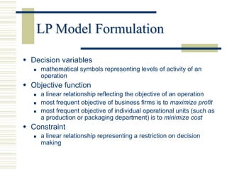
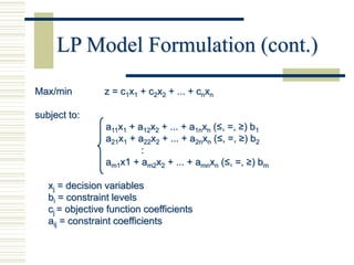
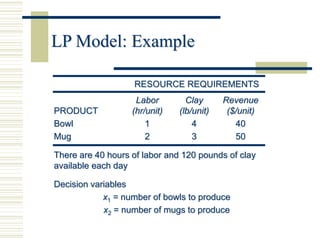
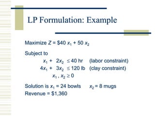
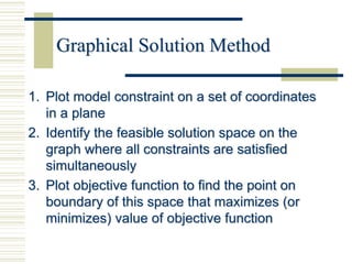
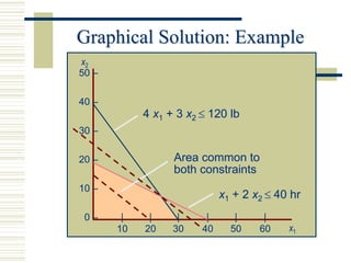
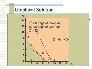
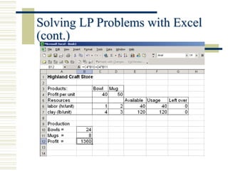
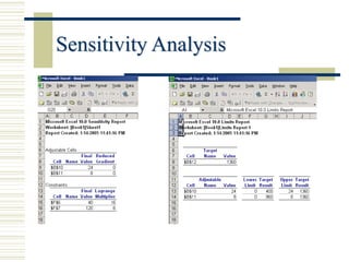
Linear programming (LP) is a mathematical modeling technique used to optimize operational activities by maximizing profit or minimizing costs under specific constraints. It involves decision variables, an objective function, and constraints which can be graphically represented to find feasible solutions. Excel can be used to solve LP problems through its solver tool, allowing for easy input of parameters and constraint management.

1. Linear Programming

2. A model consisting of linear relationships
representing a firm’s objective and resource
constraints
Linear Programming (LP)
LP is a mathematical modeling technique used to
determine a level of operational activity in order to
achieve an objective, subject to restrictions called
constraints

3. LP Model Formulation
 Decision variables
 mathematical symbols representing levels of activity of an
operation
 Objective function
 a linear relationship reflecting the objective of an operation
 most frequent objective of business firms is to maximize profit
 most frequent objective of individual operational units (such as
a production or packaging department) is to minimize cost
 Constraint
 a linear relationship representing a restriction on decision
making

4. LP Model Formulation (cont.)
Max/min z = c1x1 + c2x2 + ... + cnxn
subject to:
a11x1 + a12x2 + ... + a1nxn (≤, =, ≥) b1
a21x1 + a22x2 + ... + a2nxn (≤, =, ≥) b2
:
am1x1 + am2x2 + ... + amnxn (≤, =, ≥) bm
xj = decision variables
bi = constraint levels
cj = objective function coefficients
aij = constraint coefficients

5. LP Model: Example
Labor Clay Revenue
PRODUCT (hr/unit) (lb/unit) ($/unit)
Bowl 1 4 40
Mug 2 3 50
There are 40 hours of labor and 120 pounds of clay
available each day
Decision variables
x1 = number of bowls to produce
x2 = number of mugs to produce
RESOURCE REQUIREMENTS

6. LP Formulation: Example
Maximize Z = $40 x1 + 50 x2
Subject to
x1 + 2x2 40 hr (labor constraint)
4x1 + 3x2 120 lb (clay constraint)
x1 , x2 0
Solution is x1 = 24 bowls x2 = 8 mugs
Revenue = $1,360

7. Graphical Solution Method
1. Plot model constraint on a set of coordinates
in a plane
2. Identify the feasible solution space on the
graph where all constraints are satisfied
simultaneously
3. Plot objective function to find the point on
boundary of this space that maximizes (or
minimizes) value of objective function

8. Graphical Solution: Example
4 x1 + 3 x2 120 lb
x1 + 2 x2 40 hr
Area common to
both constraints
50 –
40 –
30 –
20 –
10 –
0 – |
10
|
60
|
50
|
20
|
30
|
40 x1
x2

9. Computing Optimal Values
x1 + 2x2 = 40
4x1 + 3x2 = 120
4x1 + 8x2 = 160
-4x1 - 3x2 = -120
5x2 = 40
x2 = 8
x1 + 2(8) = 40
x1 = 24
4 x1 + 3 x2 120 lb
x1 + 2 x2 40 hr
40 –
30 –
20 –
10 –
0 – |
10
|
20
|
30
|
40
x1
x2
Z = $50(24) + $50(8) = $1,360
24
8

10. Extreme Corner Points
x1 = 24 bowls
x2 = 8 mugs
Z = $1,360 x1 = 30 bowls
x2 = 0 mugs
Z = $1,200
x1 = 0 bowls
x2 = 20 mugs
Z = $1,000
A
B
C
|
20
|
30
|
40
|
10 x1
x2
40 –
30 –
20 –
10 –
0 –

11. 4x1 + 3x2 120 lb
x1 + 2x2 40 hr
40 –
30 –
20 –
10 –
0 –
B
|
10
|
20
|
30
|
40 x1
x2
C
A
Z = 70x1 + 20x2
Optimal point:
x1 = 30 bowls
x2 = 0 mugs
Z = $2,100
Objective Function

12. Minimization Problem
CHEMICAL CONTRIBUTION
Brand Nitrogen (lb/bag) Phosphate (lb/bag)
Gro-plus 2 4
Crop-fast 4 3
Minimize Z = $6x1 + $3x2
subject to
2x1 + 4x2  16 lb of nitrogen
4x1 + 3x2  24 lb of phosphate
x1, x2  0

13. 14 –
12 –
10 –
8 –
6 –
4 –
2 –
0 – |
2
|
4
|
6
|
8
|
10
|
12
|
14 x1
x2
A
B
C
Graphical Solution
x1 = 0 bags of Gro-plus
x2 = 8 bags of Crop-fast
Z = $24
Z = 6x1 + 3x2

14. Solving LP Problems with Excel
Click on “Tools”
to invoke “Solver.”
Objective function
Decision variables – bowls
(x1)=B10; mugs (x2)=B11
=C6*B10+D6*B11
=C7*B10+D7*B11
=E6-F6
=E7-F7

15. Solving LP Problems with Excel
(cont.)
After all parameters and constraints
have been input, click on “Solve.”
Objective function
Decision variables
C6*B10+D6*B11≤40
C7*B10+D7*B11≤120
Click on “Add” to
insert constraints

16. Solving LP Problems with Excel
(cont.)

17. Sensitivity Analysis