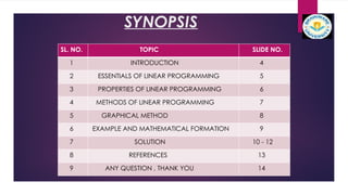
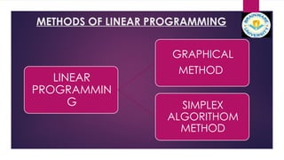
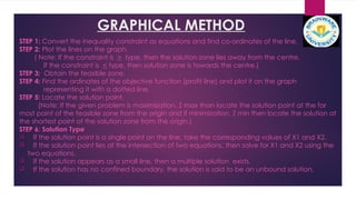
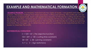
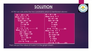
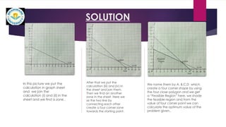
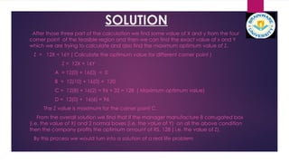
THE GRAPHICAL SOLUTION OF
LINEAR PROGRAMING PROBLEM
SUBMITTED BY
NAME: SUNITA KHAN
PROGRAM: MASTER OF LAW ( LL.M.)
SEMESTER: 1ST
STUDENT CODE: BWU/MLM/24/005
COURSE NAME : QUANTITATIVE ANALYSIS
COURSE CODE: LLM104
SUBMIITTED TO-
SUDIPTA ADHIKARY, ASST. PROFESSOR, DEPT, OF LAW
ACKNOWLEDGEMENT
I Would like to express my special thanks of gratitude to our professor, Dr. Sudipta Adhikary , Asst.
Professor, School of Law, Brainware University as well as to Dr. Kaushik Banerjee, Head of the
Department, School of Law, Brainware University who gave me the golden opportunity to do this
wonderful project on the topic The Graphical Solution of Linear Programming Problem, which also helped
me in doing a lot of research and I came to know about so many new things. I really thankful to them.
I am really indebted to my parents, who happens to be my backbone and for their untiring efforts
and the sleepless nights that they spent with me in accompanying me to carry out this project.
I also thankful to all my batch mates for their relentless support and co- operation.
Sunita Khan
LL.M, 1ST
Semester
Student Code: BWU/MLM/24/005
SYNOPSIS
SL. NO. TOPIC SLIDE NO.
1 INTRODUCTION 4
2 ESSENTIALS OF LINEAR PROGRAMMING 5
3 PROPERTIES OF LINEAR PROGRAMMING 6
4 METHODS OF LINEAR PROGRAMMING 7
5 GRAPHICAL METHOD 8
6 EXAMPLE AND MATHEMATICAL FORMATION 9
7 SOLUTION 10 - 12
8 REFERENCES 13
9 ANY QUESTION , THANK YOU 14
INTRODUCTION
Linear programming is a widely used mathematical modeling Technique to
determine the optimum allocation of scare resources among competing
demands. Resources typically include raw materials, manpower, machinery,
time, money and space.
The technique is very powerful and found especially useful because of its
application to many different types of real business problem in areas like
finance, production, sales and distribution, personnel, marketing and many
more areas of management.
As its name implies, the linear programming model consists of linear objectives
and linear constraints, which means that the variables in a model have a
proportionate relationship. For example, an increase in manpower resources will
result in increase in work output.
ESSENTIALS OF LINEAR PROGRAMMING
For a given problem situation, there are certain essential conditions that need to be solved by
using linear programming.
1. Limited Resources: Limited number of labour , material equipment and finance.
2. Objective: refers to the aim to optimize ( maximize the profits or minimize the costs).
3. Linearity: increase in labour input will have a proportionate increase in output.
4. Homogeneity: the products, workers efficiency, and machines are assumed to be
identical.
5. Divisibility: it is assumed that resources and products can be divided into fractions.
( in case the fraction are not possible, like production of one- third of a
computer, a modification of linear programming called integer
programming can be used.)
PROPERTIES OF LINEAR PROGRAMMING
THE FOLLOWING PROPERTIES FORM THE LINEAR PROGRAMING
MODEL:-
 RELATIONSHIP AMONG DECISION VARIABLES MUST BE LINEAR
IN NATURE.
 A MODEL MUST HAVE AN OBJECTIVE FUNCTION.
 RESOURCE CONSTRAINTS ARE ESSENTIAL.
 A MODEL MUST HAVE A NON- NEGATIVITY CONSTRAINTS.
METHODS OF LINEAR PROGRAMMING
LINEAR
PROGRAMMIN
G
GRAPHICAL
METHOD
SIMPLEX
ALGORITHOM
METHOD
GRAPHICAL METHOD
STEP 1: Convert the inequality constraint as equations and find co-ordinates of the line.
STEP 2: Plot the lines on the graph.
( Note: If the constraint is > type, then the solution zone lies away from the centre.
If the constraint is < type, then solution zone is towards the centre.)
STEP 3: Obtain the feasible zone.
STEP 4: Find the ordinates of the objective function (profit line) and plot it on the graph
representing it with a dotted line.
STEP 5: Locate the solution point.
(Note: If the given problem is maximization, Z max than locate the solution point at the far
most point of the feasible zone from the origin and if minimization, Z min then locate the solution at
the shortest point of the solution zone from the origin.)
STEP 6: Solution Type
 If the solution point is a single point on the line, take the corresponding values of X1 and X2.
 If the solution point lies at the intersection of two equations, then solve for X1 and X2 using the
two equations.
 If the solution appears as a small line, then a multiple solution exists.
 If the solution has no confined boundary, the solution is said to be an unbound solution.
EXAMPLE AND MATHEMATICAL FORMATION
EXAMPLE PROBLEM: A company manufacture two types of boxes, corrugated and ordinary
cartons . The boxes undergo two major processes: cutting and pinning. The profits per unit are
rs. 12 and rs.16 respectively. Each corrugated box requires 10 minutes for cutting and 8 minutes
for pinning operation, whereas each carton box requires 20 minutes for cutting and 8 minutes
for pinning. The available operating time is 120 minutes and 80 minutes for cutting and pinning
machines. The manager has to determine the optimum quantities to be manufacture the two
boxes to maximize the profits.
MATHEMATICAL FORMATION:
Z = 12X+ 16Y ( The objective function)
10X + 20Y < 120 ( cutting time constraint)
8X + 8Y < 80 ( pinning constraint)
X, Y > 0 ( Sign restrictions)
SOLUTION
At first we calculate the two constraints which is mentioned above:-
Then we put the value of X and Y in the graph sheet:-
10X + 20Y = 120
When, X= 0, Y = ?
10X + 20Y = 120
10 (0) + 20Y = 120
20Y = 120
Y = 120/ 20
Y = 6
(X = 0, Y = 6) ………… (i)
When, Y= 0, X= ?
10X + 20Y = 120
10X + 20(0) = 120
10X = 120
X = 120/ 10
X = 12
( X = 12, Y= 0) ………( ii)
8X + 8Y = 80
When, X= 0, Y= ?
8X + 8Y = 80
8(0) + 8Y = 80
8Y = 80
Y = 80/8
Y = 10
(X =0, Y = 10) ……….. (iii)
When, Y =0, X = ?
8X + 8Y = 80
8X + 8 (0) = 80
8X = 80
X = 80/8
X = 10
( X = 10, Y = 0)………..(iv)
SOLUTION
In this picture we put the
calculation in graph sheet
and we join the
calculation (i) and (ii) in the
sheet and we find a zone .
After that we put the
calculation (iii) and (iv) in
the sheet and join them.
Then we find an another
zone in the sheet. Here we
se the two line by
connecting each other
create a four corner zone
towards the starting point.
We name them by A, B,C,D which
create a four corner shape by using
the four close polygon and we get
a “Feasible Region” here. we shade
the feasible region and from the
value of four corner point we can
calculate the optimum value of the
problem given..
SOLUTION
After those three part of the calculation we find some value of X and y from the four
corner point of the feasible region and then we can find the exact value of x and Y
which we are trying to calculate and also find the maximum optimum value of Z.
Z = 12X + 16Y ( Calculate the optimum value for different corner point )
Z = 12X + 16Y
A = 12(0) + 16(0) = 0
B = 12(10) + 16(0) = 120
C = 12(8) + 16(2) = 96 + 32 = 128 ( Maximum optimum value)
D = 12(0) + 16(6) = 96
The Z value is maximum for the corner point C.
From the overall solution we find that if the manager manufacture 8 corrugated box
(i.e. the value of X) and 2 normal boxes (i.e. the value of Y) on all the above condition
then the company profits the optimum amount of RS. 128 ( i.e. the value of Z).
By this process we would turn into a solution of a real life problem
REFERENCES
 OPERATIONS RESEARCH BY V.K. KAPOOR .
 Https://www.Scribd.Com/doc/92371104/project-on-linear-programming-pr
oblems
last accessed on 17.09.2024 at 3.10 PM.
 https://www.slideteam.net/tag/linear-programming-powerpoint-templates-
ppt-slides-images-graphics-and-themes
last accessed on 18.09.2024 at 12.10 PM.
 https://youtu.be/wEkEihCorHw?si=V6ykPTYmi5JrfqTP last accessed on
18.09.2024 at 4.20 PM.
THANK YOU TO ALL

Graphical Solution in LPP along with graphs and formula

  • 1.
    THE GRAPHICAL SOLUTIONOF LINEAR PROGRAMING PROBLEM SUBMITTED BY NAME: SUNITA KHAN PROGRAM: MASTER OF LAW ( LL.M.) SEMESTER: 1ST STUDENT CODE: BWU/MLM/24/005 COURSE NAME : QUANTITATIVE ANALYSIS COURSE CODE: LLM104 SUBMIITTED TO- SUDIPTA ADHIKARY, ASST. PROFESSOR, DEPT, OF LAW
  • 2.
    ACKNOWLEDGEMENT I Would liketo express my special thanks of gratitude to our professor, Dr. Sudipta Adhikary , Asst. Professor, School of Law, Brainware University as well as to Dr. Kaushik Banerjee, Head of the Department, School of Law, Brainware University who gave me the golden opportunity to do this wonderful project on the topic The Graphical Solution of Linear Programming Problem, which also helped me in doing a lot of research and I came to know about so many new things. I really thankful to them. I am really indebted to my parents, who happens to be my backbone and for their untiring efforts and the sleepless nights that they spent with me in accompanying me to carry out this project. I also thankful to all my batch mates for their relentless support and co- operation. Sunita Khan LL.M, 1ST Semester Student Code: BWU/MLM/24/005
  • 3.
    SYNOPSIS SL. NO. TOPICSLIDE NO. 1 INTRODUCTION 4 2 ESSENTIALS OF LINEAR PROGRAMMING 5 3 PROPERTIES OF LINEAR PROGRAMMING 6 4 METHODS OF LINEAR PROGRAMMING 7 5 GRAPHICAL METHOD 8 6 EXAMPLE AND MATHEMATICAL FORMATION 9 7 SOLUTION 10 - 12 8 REFERENCES 13 9 ANY QUESTION , THANK YOU 14
  • 4.
    INTRODUCTION Linear programming isa widely used mathematical modeling Technique to determine the optimum allocation of scare resources among competing demands. Resources typically include raw materials, manpower, machinery, time, money and space. The technique is very powerful and found especially useful because of its application to many different types of real business problem in areas like finance, production, sales and distribution, personnel, marketing and many more areas of management. As its name implies, the linear programming model consists of linear objectives and linear constraints, which means that the variables in a model have a proportionate relationship. For example, an increase in manpower resources will result in increase in work output.
  • 5.
    ESSENTIALS OF LINEARPROGRAMMING For a given problem situation, there are certain essential conditions that need to be solved by using linear programming. 1. Limited Resources: Limited number of labour , material equipment and finance. 2. Objective: refers to the aim to optimize ( maximize the profits or minimize the costs). 3. Linearity: increase in labour input will have a proportionate increase in output. 4. Homogeneity: the products, workers efficiency, and machines are assumed to be identical. 5. Divisibility: it is assumed that resources and products can be divided into fractions. ( in case the fraction are not possible, like production of one- third of a computer, a modification of linear programming called integer programming can be used.)
  • 6.
    PROPERTIES OF LINEARPROGRAMMING THE FOLLOWING PROPERTIES FORM THE LINEAR PROGRAMING MODEL:-  RELATIONSHIP AMONG DECISION VARIABLES MUST BE LINEAR IN NATURE.  A MODEL MUST HAVE AN OBJECTIVE FUNCTION.  RESOURCE CONSTRAINTS ARE ESSENTIAL.  A MODEL MUST HAVE A NON- NEGATIVITY CONSTRAINTS.
  • 7.
    METHODS OF LINEARPROGRAMMING LINEAR PROGRAMMIN G GRAPHICAL METHOD SIMPLEX ALGORITHOM METHOD
  • 8.
    GRAPHICAL METHOD STEP 1:Convert the inequality constraint as equations and find co-ordinates of the line. STEP 2: Plot the lines on the graph. ( Note: If the constraint is > type, then the solution zone lies away from the centre. If the constraint is < type, then solution zone is towards the centre.) STEP 3: Obtain the feasible zone. STEP 4: Find the ordinates of the objective function (profit line) and plot it on the graph representing it with a dotted line. STEP 5: Locate the solution point. (Note: If the given problem is maximization, Z max than locate the solution point at the far most point of the feasible zone from the origin and if minimization, Z min then locate the solution at the shortest point of the solution zone from the origin.) STEP 6: Solution Type  If the solution point is a single point on the line, take the corresponding values of X1 and X2.  If the solution point lies at the intersection of two equations, then solve for X1 and X2 using the two equations.  If the solution appears as a small line, then a multiple solution exists.  If the solution has no confined boundary, the solution is said to be an unbound solution.
  • 9.
    EXAMPLE AND MATHEMATICALFORMATION EXAMPLE PROBLEM: A company manufacture two types of boxes, corrugated and ordinary cartons . The boxes undergo two major processes: cutting and pinning. The profits per unit are rs. 12 and rs.16 respectively. Each corrugated box requires 10 minutes for cutting and 8 minutes for pinning operation, whereas each carton box requires 20 minutes for cutting and 8 minutes for pinning. The available operating time is 120 minutes and 80 minutes for cutting and pinning machines. The manager has to determine the optimum quantities to be manufacture the two boxes to maximize the profits. MATHEMATICAL FORMATION: Z = 12X+ 16Y ( The objective function) 10X + 20Y < 120 ( cutting time constraint) 8X + 8Y < 80 ( pinning constraint) X, Y > 0 ( Sign restrictions)
  • 10.
    SOLUTION At first wecalculate the two constraints which is mentioned above:- Then we put the value of X and Y in the graph sheet:- 10X + 20Y = 120 When, X= 0, Y = ? 10X + 20Y = 120 10 (0) + 20Y = 120 20Y = 120 Y = 120/ 20 Y = 6 (X = 0, Y = 6) ………… (i) When, Y= 0, X= ? 10X + 20Y = 120 10X + 20(0) = 120 10X = 120 X = 120/ 10 X = 12 ( X = 12, Y= 0) ………( ii) 8X + 8Y = 80 When, X= 0, Y= ? 8X + 8Y = 80 8(0) + 8Y = 80 8Y = 80 Y = 80/8 Y = 10 (X =0, Y = 10) ……….. (iii) When, Y =0, X = ? 8X + 8Y = 80 8X + 8 (0) = 80 8X = 80 X = 80/8 X = 10 ( X = 10, Y = 0)………..(iv)
  • 11.
    SOLUTION In this picturewe put the calculation in graph sheet and we join the calculation (i) and (ii) in the sheet and we find a zone . After that we put the calculation (iii) and (iv) in the sheet and join them. Then we find an another zone in the sheet. Here we se the two line by connecting each other create a four corner zone towards the starting point. We name them by A, B,C,D which create a four corner shape by using the four close polygon and we get a “Feasible Region” here. we shade the feasible region and from the value of four corner point we can calculate the optimum value of the problem given..
  • 12.
    SOLUTION After those threepart of the calculation we find some value of X and y from the four corner point of the feasible region and then we can find the exact value of x and Y which we are trying to calculate and also find the maximum optimum value of Z. Z = 12X + 16Y ( Calculate the optimum value for different corner point ) Z = 12X + 16Y A = 12(0) + 16(0) = 0 B = 12(10) + 16(0) = 120 C = 12(8) + 16(2) = 96 + 32 = 128 ( Maximum optimum value) D = 12(0) + 16(6) = 96 The Z value is maximum for the corner point C. From the overall solution we find that if the manager manufacture 8 corrugated box (i.e. the value of X) and 2 normal boxes (i.e. the value of Y) on all the above condition then the company profits the optimum amount of RS. 128 ( i.e. the value of Z). By this process we would turn into a solution of a real life problem
  • 13.
    REFERENCES  OPERATIONS RESEARCHBY V.K. KAPOOR .  Https://www.Scribd.Com/doc/92371104/project-on-linear-programming-pr oblems last accessed on 17.09.2024 at 3.10 PM.  https://www.slideteam.net/tag/linear-programming-powerpoint-templates- ppt-slides-images-graphics-and-themes last accessed on 18.09.2024 at 12.10 PM.  https://youtu.be/wEkEihCorHw?si=V6ykPTYmi5JrfqTP last accessed on 18.09.2024 at 4.20 PM.
  • 14.