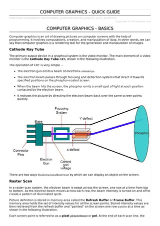
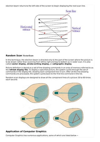
This document provides a brief overview of computer graphics. It discusses how computer graphics works by rendering images through programming computations and data manipulation. It describes the cathode ray tube as the primary output device for early graphical systems. It also summarizes two common scanning techniques - raster scan and random scan/vector scan. Additional topics covered include line generation algorithms like DDA, Bresenham's, and mid-point algorithms. It concludes with some common applications of computer graphics like GUIs, business presentations, mapping, and medical imaging.
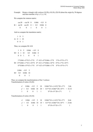


![Chapter 3 - Part 1 [Autosaved].pptx](https://cdn.slidesharecdn.com/ss_thumbnails/chapter3-part1autosaved-230109040832-9344385c-thumbnail.jpg?width=640&height=640&fit=bounds)