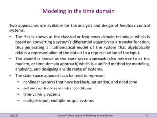
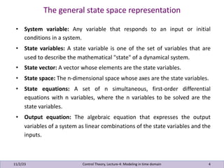
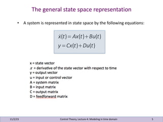
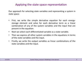
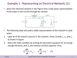
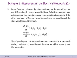
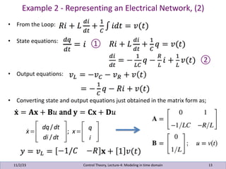
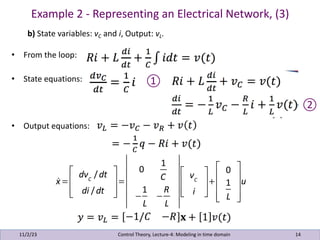
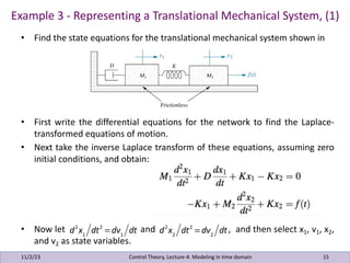
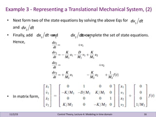
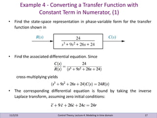
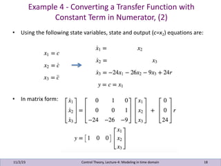
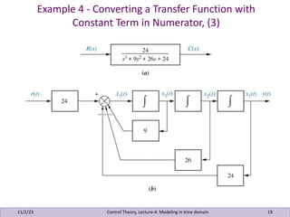
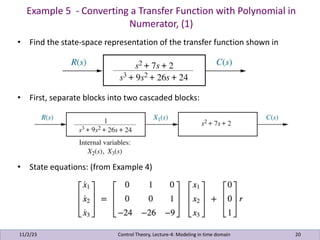
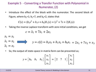
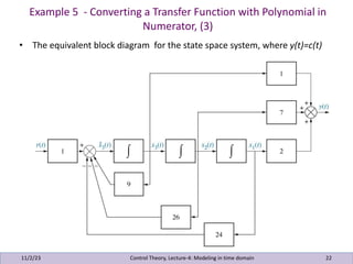
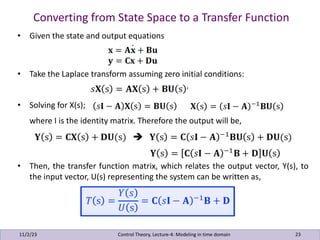
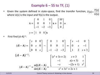
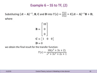
Control Theory Lecture 4: State-Space Representation

Control Theory
11/2/23 Control Theory, Lecture-4: Modeling in time domain 1
Fatma Yildiz Tascikaraoglu
Mugla Sitki Kocman Univeristy
Electrical and Electronics Engineering
fatmayildiz@mu.edu.tr,
2023-2024 / Fall semester

Lecture-4
Modeling in the time domain
11/2/23 2
Control Theory, Lecture-4: Modeling in time domain

Modeling in the time domain
11/2/23 3
Two approaches are available for the analysis and design of feedback control
systems.
• The first is known as the classical or frequency-domain technique which is
based on converting a system’s differential equation to a transfer function,
thus generating a mathematical model of the system that algebraically
relates a representation of the output to a representation of the input.
• The second is known as the state-space approach (also referred to as the
modern, or time-domain approach) which is a unified method for modeling,
analyzing, and designing a wide range of systems.
• The state-space approach can be used to represent
• nonlinear systems that have backlash, saturation, and dead zone
• systems with nonzero initial conditions
• time-varying systems
• multiple-input, multiple-output systems

The general state space representation
11/2/23 4
• System variable: Any variable that responds to an input or initial
conditions in a system.
• State variables: A state variable is one of the set of variables that are
used to describe the mathematical "state" of a dynamical system.
• State vector: A vector whose elements are the state variables.
• State space: The n-dimensional space whose axes are the state variables.
• State equations: A set of n simultaneous, first-order differential
equations with n variables, where the n variables to be solved are the
state variables.
• Output equation: The algebraic equation that expresses the output
variables of a system as linear combinations of the state variables and the
inputs.

The general state space representation
11/2/23 5
• A system is represented in state space by the following equations:
!
x(t)= Ax(t)+Bu(t)
y = Cx(t)+Du(t)

Applying the state space representation
11/2/23 6
Our approach for selecting state variables and representing a system in
state space:
• First, we write the simple derivative equation for each energy-
storage element and solve for each derivative term as a linear
combination of any of the system variables and the input that are
present in the equation.
• Next we select each differentiated variable as a state variable.
• Then we express all other system variables in the equations in terms
of the state variables and the input.
• Finally, we write the output variables as linear combinations of the
state variables and the input.

Example 1 - Representing an Electrical Network, (1)
11/2/23 7
• Given the electrical network in the Figure find a state-space representation
if the output is the current through the resistor.
• The following steps will yield a viable representation of the network in state
space.
1. Label all of the branch currents in the network. These include iL, iR, and iC,
as shown in Figure.
2. Select the state variables by writing the derivative equation for all energy
storage elements, that is, the inductor and the capacitor. Thus,
C
dVC
dt
= iC
; L
diL
dt
= vL
(1)

11/2/23 8
3. From Equations, choose the state variables as the quantities that
are differentiated, namely vC and iL. Using following equations as a
guide, we see that the state-space representation is complete if the
right-hand sides of Eqs. can be written as linear combinations of the
state variables and the input.
Since iC and vL are not state variables, our next step is to express iC
and vL as linear combinations of the state variables, vC and iL, and
the input, v(t).
dx1
(t)
dt
= a11
x1
+a12
x2
+b1
v(t)
dx2
(t)
dt
= a21
x1
+a22
x2
+b2
v(t)

11/2/23 9
4. Apply network theory, such as Kirchhoff’s voltage and current laws,
to obtain iC and vL in terms of the state variables, vC and iL. At Node
1,
(2)
which yields iC in terms of the state variables, vC and iL. Around the
outer loop,
(3)
which yields vL in terms of the state variable, vC, and the source,
v(t).
vL
= −vC
+v(t)

11/2/23 10
5. Substitute the results of Eqs. (2) and (3) into Eq. (1) to obtain the
following state equations:
(4)
6. Find the output equation. Since the output is iR(t),
(5)

11/2/23 11
• The final result for the state-space representation is found by representing
Eqs. (4) and (5) in vector-matrix form as follows:
where the dot indicates differentiation with respect to time.

11/2/23 12
• Given the electrical network in the following figure, obtain a state space
representation if the state variables are
a) Charge q(t) and current i(t)
b) Voltage accross the capacitor, vC(t) and i(t)
Select the output as the voltage accross the inductor, vL(t).
a) State variables: q and i, Output: vL.

11/2/23 13
• From the Loop:
• State equations:
• Output equations:
• Converting state and output equations just obtained in the matrix form as;
①
②
!
x =
dq/dt
di /dt
⎡
⎣
⎢
⎢
⎤
⎦
⎥
⎥
; x =
q
i
⎡
⎣
⎢
⎢
⎤
⎦
⎥
⎥

11/2/23 14
b) State variables: vC and i, Output: vL.
• From the loop:
• State equations:
• Output equations:
①
②
!
x =
dvC
/dt
di /dt
⎡
⎣
⎢
⎢
⎤
⎦
⎥
⎥
=
0
1
C
−
1
L
−
R
L
⎡
⎣
⎢
⎢
⎢
⎢
⎤
⎦
⎥
⎥
⎥
⎥
vC
i
⎡
⎣
⎢
⎢
⎤
⎦
⎥
⎥
+
0
1
L
⎡
⎣
⎢
⎢
⎢
⎤
⎦
⎥
⎥
⎥
u

• Find the state equations for the translational mechanical system shown in
• First write the differential equations for the network to find the Laplace-
transformed equations of motion.
• Next take the inverse Laplace transform of these equations, assuming zero
initial conditions, and obtain:
• Now let and , and then select x1, v1, x2,
and v2 as state variables.
Example 3 - Representing a Translational Mechanical System, (1)
11/2/23 15
d2
x1
dt2
= dv1
dt d2
x2
dt2
= dv2
dt

Example 3 - Representing a Translational Mechanical System, (2)
11/2/23 16
• Next form two of the state equations by solving the above Eqs for
and
• Finally, add and to complete the set of state equations.
Hence,
• In matrix form,
dv1
dt
dv2
dt
dx1
dt = v1
dx2
dt = v2

Example 4 - Converting a Transfer Function with
Constant Term in Numerator, (1)
11/2/23 17
• Find the state-space representation in phase-variable form for the transfer
function shown in
• Find the associated differential equation. Since
cross-multiplying yields
• The corresponding differential equation is found by taking the inverse
Laplace transform, assuming zero initial conditions:

11/2/23 18
• Using the following state variables, state and output (c=x1) equations are:
• In matrix form:

11/2/23 19

Example 5 - Converting a Transfer Function with Polynomial in
Numerator, (1)
11/2/23 20
• Find the state-space representation of the transfer function shown in
• First, separate blocks into two cascaded blocks:
• State equations: (from Example 4)

Numerator, (2)
11/2/23 21
• Introduce the effect of the block with the numerator. The second block of
Figure, where b2=1; b1=7, and b0=2, states that
• Taking the inverse Laplace transform with zero initial conditions, we get
• So, the output of state-space in matrix form can be presented as;

Numerator, (3)
11/2/23 22
• The equivalent block diagram for the state space system, where y(t)=c(t)

Converting from State Space to a Transfer Function
11/2/23 23
• Given the state and output equations
• Take the Laplace transform assuming zero initial conditions:
• Solving for X(s);
where I is the identity matrix. Therefore the output will be,
• Then, the transfer function matrix, which relates the output vector, Y(s), to
the input vector, U(s) representing the system can be written as,

Example 6 – SS to TF, (1)
11/2/23 24
• Given the system defined in state-space, find the transfer function,
where U(s) is the input and Y(s) is the output.
• First find (sI-A)-1:
T(s)=
Y(s)
U(s)

Example 6 – SS to TF, (2)
11/2/23 25

Control Theory Lecture 4: State-Space Representation

More Related Content

Similar to Control Theory Lecture 4: State-Space Representation

Recently uploaded

Control Theory Lecture 4: State-Space Representation