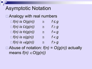
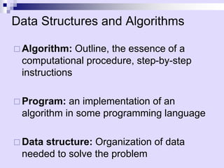
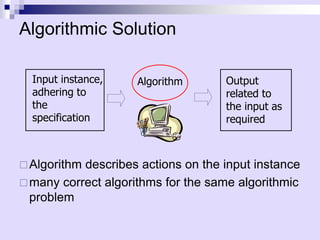
Asymptotic analysis allows the comparison of algorithms based on how their running time grows with input size rather than experimental testing. It involves analyzing an algorithm's pseudo-code to count primitive operations and expressing the running time using asymptotic notation like O(f(n)) which ignores constants. Common time complexities include constant O(1), logarithmic O(log n), linear O(n), quadratic O(n^2), and exponential O(2^n). Faster algorithms have lower asymptotic complexity.

1. Asymptotic Analysis

2. Data Structures and Algorithms
 Algorithm: Outline, the essence of a
computational procedure, step-by-step
instructions
 Program: an implementation of an
algorithm in some programming language
 Data structure: Organization of data
needed to solve the problem

3. Algorithmic problem
Infinite number of input instances satisfying the
specification.
 For eg: A sorted, non-decreasing sequence of natural
numbers of non-zero, finite length:
 1, 20, 908, 909, 100000, 1000000000.
 3.
Specification
of input
?
Specification
of output as
a function of
input

4. Algorithmic Solution
Algorithm describes actions on the input instance
many correct algorithms for the same algorithmic
problem
Input instance,
adhering to
the
specification
Algorithm Output
related to
the input as
required

5. What is a Good Algorithm?
 Efficient:
Running time
Space used
 Efficiency as a function of input size:
The number of bits in an input number
Number of data elements (numbers, points)

6. Measuring the Running Time
Experimental Study
 Write a program that implements the algorithm
 Run the program with data sets of varying size
and composition.
 Use a system call to get an accurate measure of
the actual running time.
50 100
0
t (ms)
n
10
20
30
40
50
60
How should we measure the
running time of an algorithm?

7. Limitations of Experimental Studies
It is necessary to implement and test the
algorithm in order to determine its running time.
Experiments done only on a limited set of inputs,
 may not be indicative of the running time on other
inputs not included in the experiment.
In order to compare two algorithms, the same
hardware and software environments needed

8. Beyond Experimental Studies
We will develop a general methodology for
analyzing running time of algorithms. This
approach
Uses a high-level description of the algorithm
instead of testing one of its implementations.
Takes into account all possible inputs.
Allows one to evaluate the efficiency of any
algorithm in a way that is independent of the
hardware and software environment.

9. Example
 Algorithm arrayMax(A, n):
Input: An array A storing n integers.
Output: The maximum element in A.

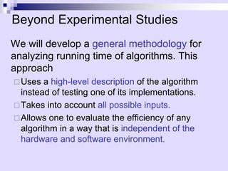
10. Pseudo-code (Functional / Recursive)
algorithm arrayMax(A[0..n-1])
{
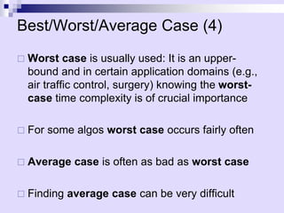
A[0] if n=1
max(arrayMax(A[0..n-2]), A[n-1]) o.w.
}

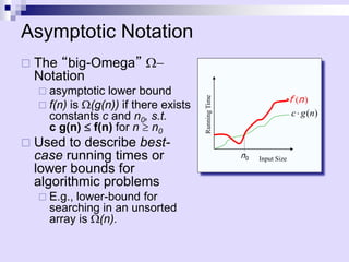
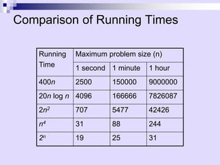
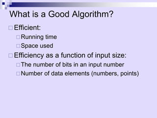
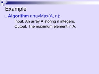
11. Pseudo-Code (imperative)
 A mixture of natural language and high-level
programming concepts that describes the main
ideas behind a generic implementation of a data
structure or algorithm.
 Eg: algorithm arrayMax(A, n):
Input: An array A storing n integers.
Output: The maximum element in A.
currentMax  A[0]
for i  1 to n-1 do
if currentMax < A[i] then currentMax  A[i]
return currentMax

12. Pseudo-Code
It is more structured than usual prose but
less formal than a programming language
 Expressions:
 use standard mathematical symbols to
describe numeric and boolean expressions
 use  for assignment (“=” in Java)
 use = for equality relationship (“==” in Java)
 Method Declarations:
 algorithm name(param1, param2)

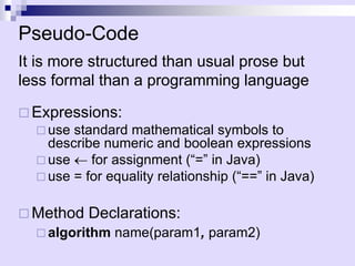
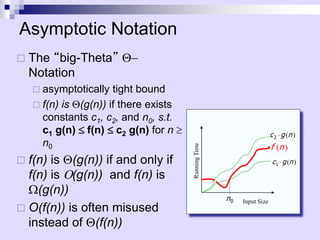
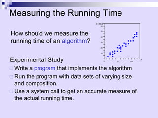
13. Pseudo Code
 Programming Constructs:
decision structures: if ... then ... [else ... ]
while-loops: while ... do
repeat-loops: repeat ... until ...
for-loop: for ... do
array indexing: A[i], A[i,j]
 Methods:
calls: object method(args)
returns: return value

14. Analysis of Algorithms
 Primitive Operation: Low-level operation
independent of programming language.
Can be identified in pseudo-code. For eg:
Data movement (assign)
Control (branch, subroutine call, return)
arithmetic an logical operations (e.g. addition,
comparison)
 By inspecting the pseudo-code, we can
count the number of primitive operations
executed by an algorithm.

15. Sort
Example: Sorting
INPUT
sequence of numbers
a1, a2, a3,….,an
b1,b2,b3,….,bn
OUTPUT
a permutation of the
sequence of numbers
2 5 4 10 7 2 4 5 7 10
Correctness (requirements for the
output)
For any given input the algorithm
halts with the output:
• b1 < b2 < b3 < …. < bn
• b1, b2, b3, …., bn is a
permutation of a1, a2, a3,….,an
Running time
Depends on
• number of elements (n)
• how (partially) sorted
they are
• algorithm

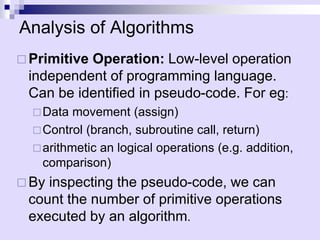
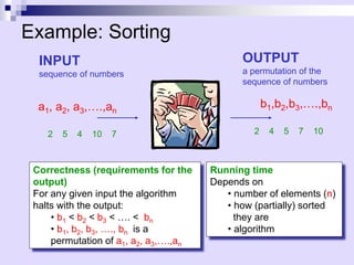
16. Insertion Sort
A
1 n
j
3 6 8
4 9 7 2 5 1
i
Strategy
• Start “empty handed”
• Insert a card in the right
position of the already sorted
hand
• Continue until all cards are
inserted/sorted
INPUT: A[0..n-1] – an array of integers
OUTPUT: a permutation of A such that
A[0]A[1]…A[n-1]

17. Pseudo-code (Functional / Recursive)
algorithm insertionSort(A[0..n-1])
{
A[0] if n=1
insert(insertionSort(A[0..n-2]), A[n-1]) o.w.
}
algorithm insert(A[0..n-1], key)
{
append(A[0..n-1], key) if key>=A[n-1]
append(newarray(key), A[0]) if n=1&key<A[0]
append(insert(A[0..n-2],key), A[n-1]) o.w.
}

18. Insertion Sort
A
1 n
j
3 6 8
4 9 7 2 5 1
i
Strategy
• Start “empty handed”
• Insert a card in the right
position of the already sorted
hand
• Continue until all cards are
inserted/sorted
INPUT: A[0..n-1] – an array of integers
OUTPUT: a permutation of A such that
A[0]A[1]…A[n-1]
for j1 to n-1 do
key A[j]
//insert A[j] into the sorted sequence
A[0..j-1]
ij-1
while i>=0 and A[i]>key
do A[i+1]A[i]
i--
A[i+1]key

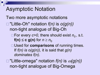
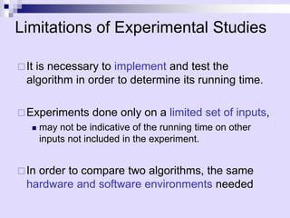
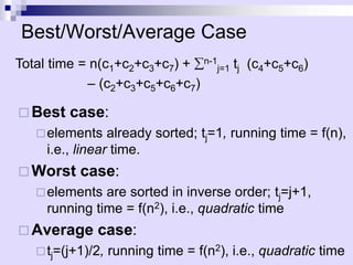
19. Analysis of Insertion Sort
for j1 to n-1 do
keyA[j]
//insert A[j] into the sorted
sequence A[0..j-1]
ij-1
while i>=0 and A[i]>key
do A[i+1]A[i]
i--
A[i+1]  key
cost
c1
c2
0
c3
c4
c5
c6
c7
Times
n
n-1
n-1
n-1
n-1
Total time = n(c1+c2+c3+c7) + n-1
j=1 tj (c4+c5+c6)
– (c2+c3+c5+c6+c7)
𝒋=𝟏
𝒏−𝟏
𝒕𝒋
𝒋=𝟏
𝒏−𝟏
(𝒕𝒋 − 𝟏)
𝒋=𝟏
𝒏−𝟏
(𝒕𝒋 − 𝟏)

20. Best/Worst/Average Case
 Best case:
elements already sorted; tj=1, running time = f(n),
i.e., linear time.
 Worst case:
elements are sorted in inverse order; tj=j+1,
running time = f(n2), i.e., quadratic time
 Average case:
tj=(j+1)/2, running time = f(n2), i.e., quadratic time
Total time = n(c1+c2+c3+c7) + n-1
j=1 tj (c4+c5+c6)
– (c2+c3+c5+c6+c7)

21. Best/Worst/Average Case (2)
 For a specific size of input n, investigate
running times for different input instances:

22. Best/Worst/Average Case (3)
For inputs of all sizes:
1n
2n
3n
4n
5n
6n
Input instance size
Running
time
1 2 3 4 5 6 7 8 9 10 11 12 …..
best-case
average-case
worst-case

23. Best/Worst/Average Case (4)
 Worst case is usually used: It is an upper-
bound and in certain application domains (e.g.,
air traffic control, surgery) knowing the worst-
case time complexity is of crucial importance
 For some algos worst case occurs fairly often
 Average case is often as bad as worst case
 Finding average case can be very difficult

24. Asymptotic Analysis
 Goal: to simplify analysis of running time by
getting rid of ”details”, which may be affected by
specific implementation and hardware
 like “rounding”: 1,000,001  1,000,000
 3n2  n2
 Capturing the essence: how the running time of
an algorithm increases with the size of the input
in the limit.
 Asymptotically more efficient algorithms are best for
all but small inputs

25. Asymptotic Notation
 The “big-Oh” O-Notation
asymptotic upper bound
f(n) is O(g(n)), if there exists constants c and n0,
s.t. f(n)  c g(n) for all n  n0
f(n) and g(n) are functions over non-negative
integers
 Used for worst-case
analysis
)
(n
f
( )
c g n

0
n Input Size
Running
Time

26. Example
f(n) =2n +6
For functions f(n) and g(n) there are positive
constants c and n0 such that: f(n) ≤ c g(n) for n ≥ n0
conclusion:
2n+6 is O(n).

27. Another Example
On the other hand…
n2 is not O(n) because there is
no c and n0 such that:
n2 ≤ cn for n ≥ n0
The graph to the right
illustrates that no matter how
large a c is chosen there is an n
big enough that n2 > cn ) .

28. Asymptotic Notation
 Simple Rule: Drop lower order terms and
constant factors.
50 n log n is O(n log n)
7n - 3 is O(n)
8n2 log n + 5n2 + n is O(n2 log n)
 Note: Even though (50 n log n) is O(n5), it
is expected that such an approximation be
of as small an order as possible

29. Asymptotic Analysis of Running Time
 Use O-notation to express number of primitive
operations executed as function of input size.
 Comparing asymptotic running times
an algorithm that runs in O(n) time is better
than one that runs in O(n2) time
similarly, O(log n) is better than O(n)
hierarchy of functions: log n < n < n2 < n3 < 2n
 Caution! Beware of very large constant factors.
An algorithm running in time 1,000,000 n is still
O(n) but might be less efficient than one running
in time 2n2, which is O(n2)

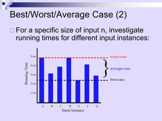
30. Example of Asymptotic Analysis
Algorithm prefixAverages1(X):
Input: An n-element array X of numbers.
Output: An n-element array A of numbers such that
A[i] is the average of elements X[0], ... , X[i].
for i  0 to n-1 do
a  0
for j  0 to i do
a  a + X[j]
A[i]  a/(i+1)
return array A
Analysis: running time is O(n2)
1 step
i iterations
with
i=0,1,2...n-1
n iterations

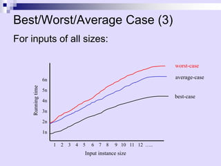
31. A Better Algorithm
Algorithm prefixAverages2(X):
Input: An n-element array X of numbers.
Output: An n-element array A of numbers such
that A[i] is the average of elements X[0], ... , X[i].
s  0
for i  0 to n do
s  s + X[i]
A[i]  s/(i+1)
return array A
Analysis: Running time is O(n)

32. Asymptotic Notation (terminology)
 Special classes of algorithms:
 Logarithmic: O(log n)
 Linear: O(n)
 Quadratic: O(n2)
 Polynomial: O(nk), k ≥ 1
 Exponential: O(an), a > 1
 “Relatives” of the Big-Oh
  (f(n)): Big Omega -asymptotic lower bound
  (f(n)): Big Theta -asymptotic tight bound

33.  The “big-Omega” -
Notation
 asymptotic lower bound
 f(n) is (g(n)) if there exists
constants c and n0, s.t.
c g(n)  f(n) for n  n0
 Used to describe best-
case running times or
lower bounds for
algorithmic problems
 E.g., lower-bound for
searching in an unsorted
array is (n).
Input Size
Running
Time
)
(n
f
( )
c g n

0
n
Asymptotic Notation

34.  The “big-Theta” -
Notation
 asymptotically tight bound
 f(n) is (g(n)) if there exists
constants c1, c2, and n0, s.t.
c1 g(n)  f(n)  c2 g(n) for n 
n0
 f(n) is (g(n)) if and only if
f(n) is O(g(n)) and f(n) is
(g(n))
 O(f(n)) is often misused
instead of (f(n))
Asymptotic Notation
Input Size
Running
Time
)
(n
f
0
n
)
(n
g
c 
2
)
(n
g
c 
1

35. Asymptotic Notation
Two more asymptotic notations
 "Little-Oh" notation f(n) is o(g(n))
non-tight analogue of Big-Oh
For every c>0, there should exist n0 , s.t.
f(n)  c g(n) for n  n0
Used for comparisons of running times.
If f(n) is o(g(n)), it is said that g(n)
dominates f(n).
 "Little-omega" notation f(n) is w(g(n))
non-tight analogue of Big-Omega

36. Asymptotic Notation
 Analogy with real numbers
f(n) is O(g(n)) @ f g
f(n) is (g(n)) @ f  g
f(n) is (g(n)) @ f =g
f(n) is o(g(n)) @ f <g
f(n) is w(g(n)) @ f >g
 Abuse of notation: f(n) = O(g(n)) actually
means f(n) O(g(n))

37. Comparison of Running Times
Running
Time
Maximum problem size (n)
1 second 1 minute 1 hour
400n 2500 150000 9000000
20n log n 4096 166666 7826087
2n2 707 5477 42426
n4 31 88 244
2n 19 25 31