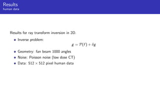
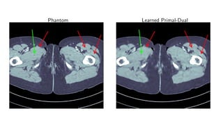
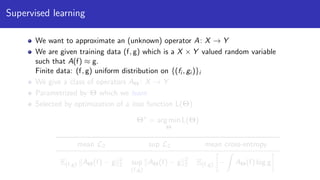
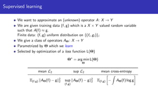
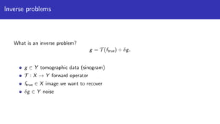
1) Machine learning techniques can be used to learn priors for solving inverse problems like image reconstruction from limited data.
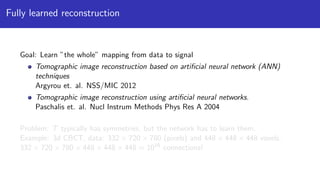
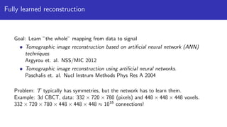
2) Fully learned reconstruction is infeasible due to the large number of parameters needed. Learned post-processing and learned iterative reconstruction methods provide better results.
3) Learned iterative reconstruction formulates the problem as learning updating operators in an iterative optimization scheme, but is computationally challenging due to the need to differentiate through the whole solver. Future work includes methods to address this issue.


![Example: L2 loss
Example: L2-loss of reconstruction
L(Θ) = E(f,g)∼µ
1
2
T †
Θ(g) − f
2
X
.
(g, f)-µ distributed training data (e.g. high dose CTs, simulation)
”Learning” by Stochastic Gradient Descent (SGD):
Θi+1 = Θi − α L(Θi )
With the above loss:
L(Θ) = E(f,g)∼µ [∂Θ T †
Θ(g)]∗
T †
Θ(g) − f
Observation: The reconstruction operator must be differentiable w.r.t Θ!](https://image.slidesharecdn.com/presentationen-171006141758/85/Learning-to-Reconstruct-20-320.jpg)
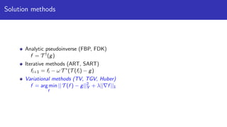
![Learned iterative reconstruction
Problem: Data g ∈ Y , reconstruction f ∈ X
How to include data in each iteration?
Inspiration from iterative optimization methods
f = arg min || T (f ) − g||2
Y
Algorithm 1 Generic gradient based optimization algorithm
1: for i = 1, . . . do
2: fi+1 ← BetterGuess fi , [∂ T (fi )]∗
(T (f ) − g)
Gradient descent:
BetterGuess fi , [∂ T (fi )]∗
(T (fi ) − g) = fi − α[∂ T (fi )]∗
(T (fi ) − g)](https://image.slidesharecdn.com/presentationen-171006141758/85/Learning-to-Reconstruct-29-320.jpg)
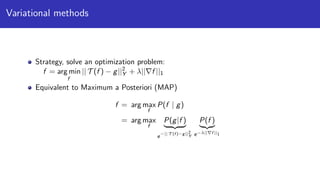
![Learned gradient descent
Set a stopping criteria (fixed number of steps)
Learn the function BetterGuess
Algorithm 2 Learned gradient descent
1: for i = 1, . . . , I do
2: f i+1
← ΛΘ fi , [∂ T (fi )]∗
(T (fi ) − g)
3: T †
Θ(g) ← fI
We separate problem dependent (and possibly global) into [∂ T (fi )]∗
(T (fi ) − g), and
local into ΛΘ!](https://image.slidesharecdn.com/presentationen-171006141758/85/Learning-to-Reconstruct-30-320.jpg)
![Structure of updating operators
What is a natural structure of ΛΘ?
Requirements:
Fast to compute
Span a rich set of functions
Easy to evaluate [∂ΘΛΘ]∗
Standard answer:
ΛΘ = WΘ1 ◦ ρ ◦ WΘ2 ◦ ρ · · · ◦ ρ ◦ WΘn
ρ pointwise nonlinearity
WΘi
affine operator](https://image.slidesharecdn.com/presentationen-171006141758/85/Learning-to-Reconstruct-31-320.jpg)
![Structure of updating operators
What class of affine operators should we use?
Some options:
Any affine operator X → X: ”Fully connected layer”
Any translational invariant operator X → X: ”Convolutional layer”
Fully connected layers are ”stronger” but require far more parameters.
In several (CT, MRI) applications, [∂ T (fi )]∗
◦ T is (approximately) translation
invariant!](https://image.slidesharecdn.com/presentationen-171006141758/85/Learning-to-Reconstruct-32-320.jpg)

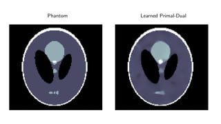
![Learned Primal-Dual algorithm
Algorithm 3 Learned Primal-Dual
1: for i = 1, . . . , I do
2: hi ← ΓΘd
i
hi−1, K(f
(2)
i−1), g
3: fi ← ΛΘp
i
fi−1, [∂ K(f
(1)
i−1)]∗
(h
(1)
i )
4: T †
Θ(g) ← f
(1)
I
Learning:
L(Θ) = Eµ T †
Θ(g) − f
2
X
.](https://image.slidesharecdn.com/presentationen-171006141758/85/Learning-to-Reconstruct-34-320.jpg)