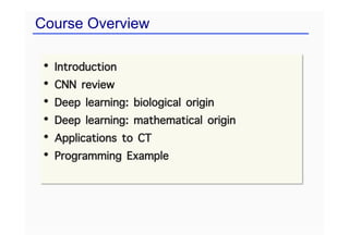
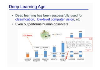
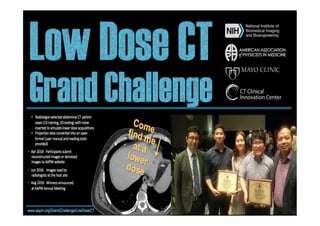
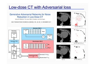
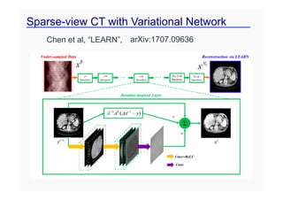
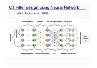
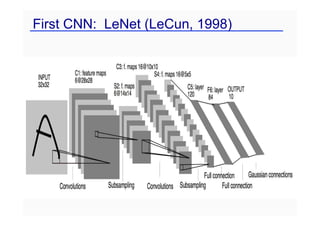
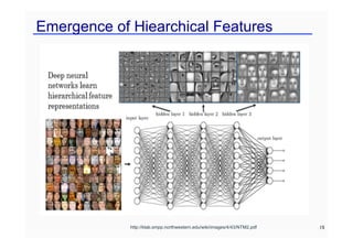
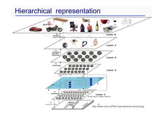
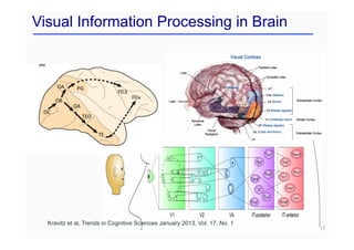
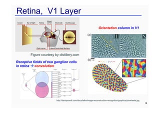
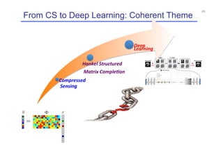
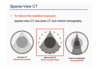
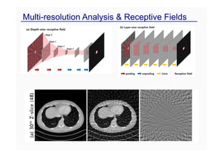
This document provides an overview of a refresher course on deep learning for CT reconstruction. The course covers an introduction to CNNs, the biological and mathematical origins of deep learning, and various applications of deep learning to CT reconstruction problems like low-dose CT, sparse-view CT, and interior tomography. Successful demonstrations of deep learning approaches for these image reconstruction problems are highlighted from recent works. The role of convolutional and pooling layers in CNNs is discussed. Reasons for why deep learning works well for reconstruction problems are explored, including the mathematical understanding of CNNs in terms of deep convolutional framelets and the lifting of signals to higher dimensional spaces using Hankel matrices. The document concludes by discussing some open problems and providing information on datasets

1. Jong Chul Ye
Bio-Imaging & Signal Processing Lab.
Dept. Bio & Brain Engineering
Dept. Mathematical Sciences
KAIST, Korea
Refresher Course
Deep Learning for CT Reconstruction:
From Concept to Practices
This can be downloaded from http://bispl.weebly.com

2. Course Overview
• Introduction
• CNN review
• Deep learning: biological origin
• Deep learning: mathematical origin
• Applications to CT
• Programming Example

3. Deep Learning Age
• Deep learning has been successfully used for
classification, low-level computer vision, etc
• Even outperforms human observers

4. 3

5. Low-dose CT with Adversarial loss

6. Sparse-view CT with Variational Network
Chen et al, “LEARN”, arXiv:1707.09636

7. CT Filter design using Neural Network
Würfl, Tobias, et al. 2016.

8. • Successful demonstra5on of deep learning for various image
reconstruc5on problems
– Low-dose x-ray CT (Kang et al, Chen et al, Wolterink et al)
– Sparse view CT (Jin et al, Han et al, Adler et al)
– Interior tomography (Han et al)
– Stationary CT for baggage inspection (Han et al)
– CS-MRI (Hammernik et al, Yang et al, Lee et al, Zhu et al)
– US imaging (Yoon et al )
– Diffuse optical tomography (Yoo et al)
– Elastic tomography (Yoo et al)
– etc
• Advantages
– Very fast reconstruction time
– Significantly improved results
Other works

9. WHY DEEP LEARNING WORKS
FOR RECON ?
DOES IT CREATE ANY
ARTIFICIAL FEATURES ?

10. First CNN: LeNet (LeCun, 1998)

11. Convolutional Layer

12. Pooling Layer
Figure from Leonardo Araujo Aantos

13. Too Simple to Analyze..
Convolution & pooling à stone age tools of signal processing
What do they do ?

14. Dark Age of Applied Mathematics ?

15. CNN – BIOLOGICAL ORIGIN
A LAYMAN’S EXPLANATION

16. 15
http://klab.smpp.northwestern.edu/wiki/images/4/43/NTM2.pdf
Emergence of Hiearchical Features

17. 16
http://www.vicos.si/File:Lhop-hierarchy-second.jpg
• LeCun et al, Nature, 2015
Hierarchical representation

18. Visual Information Processing in Brain
17
Kravitz et al, Trends in Cognitive Sciences January 2013, Vol. 17, No. 1

19. Retina, V1 Layer
18
Receptive fields of two ganglion cells
in retina à convolution
Orientation column in V1
http://darioprandi.com/docs/talks/image-reconstruction-recognition/graphics/pinwheels.jpg
Figure courtesy by distillery.com

20. “The Jennifer Anniston Cell”
19
Quiroga et al, Nature, Vol 435, 24, June 2005

21. 20

22. CNN – MATHEMATICAL
UNDERSTANDING

23. Why Deep Learning works for recon ?
Existing views 1: unfolded iteration
• Most prevailing views
• Direct connec5on to sparse recovery
– Cannot explain the filter channels
Jin, arXiv:1611.03679

24. Why Deep Learning works for recon ?
Existing views 2: generative model
• Image reconstruc5on as a distribu5on matching
– However, difficult to explain the role of black-box network
Bora et al, Compressed Sensing using Generative Models, arXiv:1703.03208

25. Our Proposal:
Deep Learning == Deep Convolutional
Framelets
• Ye et al, “Deep convolutional framelets: A general deep
learning framework for inverse problems”, SIAM Journal
Imaging Sciences, 11(2), 991-1048, 2018.

26. Matrix Representation of CNN
Figure courtesy of Shoieb et al, 2016

27. Hankel Matrix:
Lifting to Higher Dimensional Space

28. Why we are excited about Hankel matrix ?
T
-T 0
n1
-n1 0
* FRI Sampling theory (VeEerlie et al) and compressed sensing

29. ︙
︙
1
2
3
4
5
6
7
8
9
-1
0 1
2
3
4
5
6
7
8
9
1
2
3
4
5
6
7
8
9
12
2
3
4
5
6
7
8
9
12
13
3
4
5
6
7
8
9
10
10
10
10
0
11
11
11
1
2
3
4
5
Finite length convolution
Matrix
Representation
* ALOHA : Annihilating filter based LOw rank Hankel matrix Approach
* Jin KH et al. IEEE TCI, 2016 * Jin KH et al.,IEEE TIP, 2015
* Ye JC et al. IEEE TIT, 2016
Annihilating filter-based low-rank Hankel matrix

30. Missing elements can be found by low rank Hankel structured matrix comple5on
Nuclear norm Projec5on on sampling posi5ons
min
m
kH(m)k⇤
subject to P⌦(b) = P⌦(f)
RankH(f) = k
* Jin KH et al IEEE TCI, 2016
* Jin KH et al.,IEEE TIP, 2015
* Ye JC et al., IEEE TIT, 2016
m
Annihilating filter-based low-rank Hankel matrix

31. Algorithmic Flow

32. 18. APR. 2015. 31
*
Image Inpainting Results

33. 32

34. Low-rank Hankel matrix in Image

35. 18. APR. 2015. 34
Algorithmic Flow
ALOHA
Computationally
Heavy

36. Key Observation
Data-Driven Hankel matrix decomposition
=> Deep Learning
• Ye et al, “Deep convolutional framelets: A general deep
learning framework for inverse problems”, SIAM Journal
Imaging Sciences, 11(2), 991-1048, 2018.

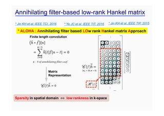
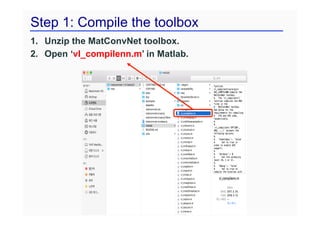
37. Hd(f) Hd(f)
= ˜T
˜ T C
C = T
Hd(f)
C = T
(f ~ )
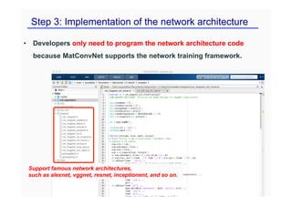
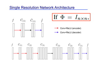
Encoder:
˜ T
= I
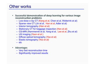
˜ = PR(V )
Hd(f) = U⌃V T
Unlifting: f = (˜C) ~ ⌧(˜)
: Non-local basis
: Local basis
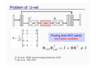
: Frame condition
: Low-rank condition
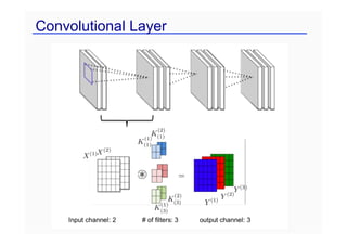
convolution
pooling
un-pooling
convolution
: User-defined pooling
: Learnable filters
Hpi
(gi) =
X
k,l
[Ci]kl
e
Bkl
i
Decoder:
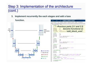
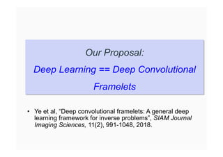
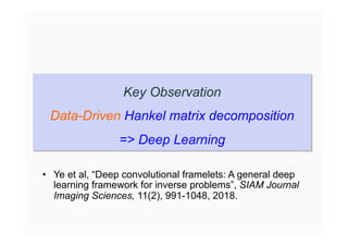
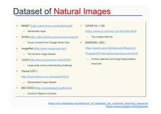
Deep Convolutional Framelets (Y, Han, Cha; 2018)

38. Single Resolution Network Architecture

39. Multi-Resolution Network Architecture

40. Role of ReLU: Conic encoding
D. D. Lee and H. S. Seung, Nature, 1999
ReLU: positive framelet
coefficients
Conic encoding à part by
representation similar to visual
cortex

41. https://www.youtube.com/watch?v=DdC0QN6f3G4
Relativity:
Lifting to the Space-time
à linear trajectory
High Dimensional Lifting in Relativity
Falling apple
Apple at rest
Universal law of gravity:
3-D Space
à curved trajectory
Falling apple
Apple at rest

42. Compressed
Sensing
Hankel Structured
Matrix Comple7on
Deep
Learning
49
From CS to Deep Learning: Coherent Theme

43. DEEP NETWORKS FOR CT

44. Low-Dose CT
• To reduce the radiation exposure,
sparse-view CT, low-dose CT and interior tomography.
Sparse-view CT
(Down-sampled View)
Low-dose CT
(Reduced X-ray dose)
Interior Tomography
(Truncated FOV)

45. 52
Wavelet
transform
level 2
level 1 level 3 level 4
Wavelet
recomposition
+
Residual learning
: Low-resolution image bypass
High SNR band
CNN
(Kang, et al, Medical Physics 44(10))

46. Routine dose Quarter dose
(Kang, et al, Medical Physics 44(10) 2017)

47. Routine dose AAPM-Net results
(Kang, et al, Medical Physics 44(10) 2017)

48. WavResNet results
(Kang et al, TMI, 2018)

49. WavResNet results
(Kang et al, TMI, 2018)

50. MBIR Our latest Result
C D WavResNet results

51. Full dose Quarter dose

52. Full dose Quarter dose

53. Sparse-View CT
• To reduce the radiation exposure,
sparse-view CT, low-dose CT and interior tomography.
Sparse-view CT
(Down-sampled View)
Low-dose CT
(Reduced X-ray dose)
Interior Tomography
(Truncated FOV)

54. Multi-resolution Analysis & Receptive Fields

55. Problem of U-net
Pooling does NOT satisfy
the frame condition
JC Ye et al, SIAM Journal Imaging Sciences, 2018
Y. Han et al, TMI, 2018.
ext
>
ext = I + >
6= I

56. Improving U-net using Deep Conv Framelets
• Dual Frame U-net
• Tight Frame U-net
JC Ye et al, SIAM Journal Imaging Sciences, 2018
Y. Han and J. C. Ye, TMI, 2018

57. U-Net versus Dual Frame U-Net

58. Tight-Frame U-Net
JC Ye et al, SIAM Journal Imaging Sciences, 2018
Han et al, TMI, 2018

59. 90 view recon
U-Net vs. Tight-Frame U-Net
• JC Ye et al, SIAM Journal
Imaging Sciences, 2018
• Y. Han and J. C. Ye, TMI,
2018

62. • Figures from internet
9 View CT for Baggage Screening

63. 9 View CT for Baggage Screening

64. 1st view 2nd view 3rd view
4th view 5th view 6th view
7th view 8th view 9th view

65. FBP

66. TV

67. Ours

68. ROI Reconstruction
• To reduce the radiation exposure,
sparse-view CT, low-dose CT and interior tomography.
Sparse-view CT
(Down-sampled View)
Low-dose CT
(Reduced X-ray dose)
Interior Tomography
(Truncated FOV)

69. Deep Learning Interior Tomography
Han et al, arXiv preprint arXiv:1712.10248, (2017): CT meeting 2018.

70. Ground
Truth
FBP

71. TV
Chord
Line
Ours
8~10 dB
gain

72. Ground
Truth
Chord
Line
TV
Ours

73. Still Unresolved Problems..
• Cascaded geometry of deep neural network
• Generalization capability
• Optimization landscape
• Training procedure
• Extension to classification problems

74. DEEP LEARNING - PRACTICES

75. Dataset of Natural Images
• MNIST (http://yann.lecun.com/exdb/mnist/)
– Handwritten digits.
• SVHN (http://ufldl.stanford.edu/housenumbers/)
– House numbers from Google Street View.
• ImageNet (http://www.image-net.org/)
– The de-facto image dataset.
• LSUN (http://lsun.cs.princeton.edu/2016/)
– Large-scale scene understanding challenge.
• Pascal VOC (
http://host.robots.ox.ac.uk/pascal/VOC/)
– Standardized image dataset.
• MS COCO (http://cocodataset.org/#home)
– Common Objects in Context.
• CIFAR-10 / -100
(https://www.cs.utoronto.ca/~kriz/cifar.html)
– Tiny images data set.
• BSDS300 / 500 (
https://www2.eecs.berkeley.edu/Research/
Projects/CS/vision/grouping/resources.html)
– Contour detection and image Segmentation
resources.
https://en.wikipedia.org/wiki/List_of_datasets_for_machine_learning_research
https://www.kaggle.com/datasets

76. Dataset for Medical Images
• HCP (https://www.humanconnectome.org/)
– Behavioral and 3T / 7T MR imaging dataset.
• MRI Data (http://mridata.org/)
– Raw k-space dataset acquired on
a GE clinical 3T scanner.
• LUNA (https://luna16.grand-challenge.org/data/)
– Lung Nodule analysis dataset acquired on a CT scanner.
• Data Science Bowl
(https://www.kaggle.com/c/data-science-bowl-2017)
– A thousand low-dose CT images.
• NIH Chest X-rays
(https://nihcc.app.box.com/v/ChestXray-NIHCC)
– X-ray images with disease labels.
http://www.cancerimagingarchive.net/
https://www.kaggle.com/datasets
• TCIA Collections
(http://www.cancerimagingarchive.net/)
• De-identifies and hosts a large archive of medical
images of
cancer accessible for public download.
• The data are organized as “Collections”, typically
patients related
by a common disease, image modality (MRI, CT,
etc).

77. Libraries for Deep learning
• TensorFlow (https://www.tensorflow.org/)
– Python
• Theano (
http://deeplearning.net/software/theano/)
– Python
• Keras (https://keras.io/)
– Python
• Caffe (http://caffe.berkeleyvision.org/)
– Python
• Torch (or PyTorch) (http://torch.ch/)
– C / C++ (or Python)
• Deeplearning4J (
https://deeplearning4j.org/)
– Java
• Microsoft Cognitive Toolkit (CNTK)
(
https://www.microsoft.com/en-us/cognitive-
toolkit/)
– Python / C / C++
• MatConvNet (
http://www.vlfeat.org/matconvnet/)
– Matlab

78. Implementation on MatConvNet
Download
the
MatConvNet
Provide the
pre-trained
models

79. Step 1: Compile the toolbox
1. Unzip the MatConvNet toolbox.
2. Open ‘vl_compilenn.m’ in Matlab.

80. Step 1: Compile the toolbox (cont.)
3. Check the options such as enableGpu and enableCudnn.
4. Run the ‘vl_compilenn.m’.
* To use GPU processing (false true),
you must have CUDA installed.
( https://developer.nvidia.com/cuda-90-download-archive )
** To use cuDNN library (false true),
you must have cuDNN installed.
( https://developer.nvidia.com/cudnn )

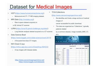
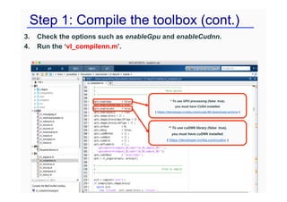
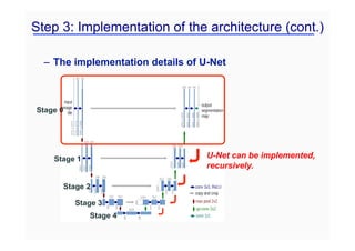
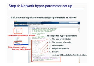
81. Step 2: Prepare dataset
As a classification example, MNIST consists of as follows,
Images % struct-type
Data % handwritten digit image
labels % [1, …, 10]
set % [1, 2, 3],
1, 2, and 3 indicate
train, valid, and test set, respectively.
Data Labels
6

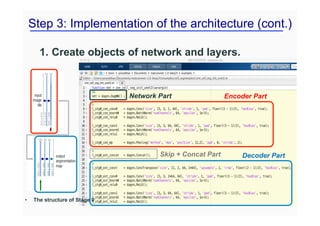
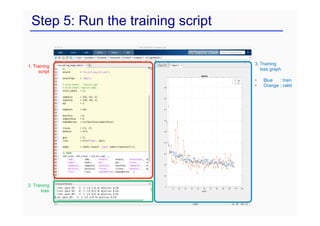
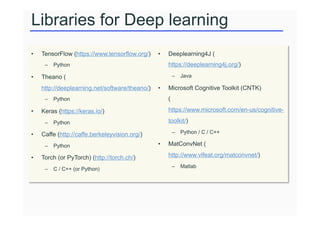
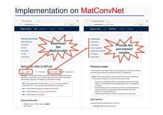
82. Step 2: Prepare dataset (cont.)
• As a segmentation example, U-Net dataset consists of as follows,
– Images % struct-type
Ø data % Cell image
Ø labels % [1, 2], Mask image.
1 and 2 indicate
back- and for-ground, respectively.
Ø set % [1, 2, 3]
Data Labels

83. Step 3: Implementation of the network architecture
• Developers only need to program the network architecture code
because MatConvNet supports the network training framework.
Support famous network architectures,
such as alexnet, vggnet, resnet, inceptionent, and so on.

84. Step 3: Implementation of the architecture (cont.)
– The implementation details of U-Net
U-Net can be implemented,
recursively.
Stage 0
Stage 1
Stage 2
Stage 3
Stage 4

85. Step 3: Implementation of the architecture (cont.)
1. Create objects of network and layers.
Encoder Part
Skip + Concat Part Decoder Part
• The structure of Stage 0
Network Part

86. Step 3: Implementation of the architecture (cont.)
2. Connect each layers.
• The structure of Stage 0
Layer Name
( string-type )
Layer object
( object )
Input Name
( string-type )
Output Name
( string-type )
Parameters Name
( string-type )
All objects and names must be unique.

87. Step 3: Implementation of the architecture
(cont.)
3. Implement recurrently the each stages and add a loss
function.
Previous parts (3.1 and 3.2)
become functional as
‘add_block_unet’.

88. Step 4: Network hyper-parameter set up
• MatConvNet supports the default hyper-parameters as follows,
Refer the cnn_train.m
( or cnn_train_dag.m )
The supported hyper-parameters
1. The size of mini-batch
2. The number of epochs
3. Learning rate
4. Weight decay factor
5. Solvers
such as SGD, AdaDelta, AdaGrad, Adam, and RMS
The kind of Optimization Solvers

89. Step 5: Run the training script
1. Training
script
2. Training
loss
3. Training
loss graph
• Blue : train
• Orange : valid

90. Acknowledgements
CT Team
• Yoseob Han
• Eunhee Kang
• Jawook Goo
US Team
• Shujaat Khan
• Jaeyong Hur
MR Team
• Dongwook Lee
• Juyoung Lee
• Eunju Cha
• Byung-hoon Kim
Image Analysis Team
• Boa Kim
• Junyoung Kim
Optics Team
• Sungjun Lim
• Junyoung Kim
• Jungsol Kim
• Taesung Kwon

91. THANK YOU
This presentation material can be downloaded from
http://bispl.weebly.com