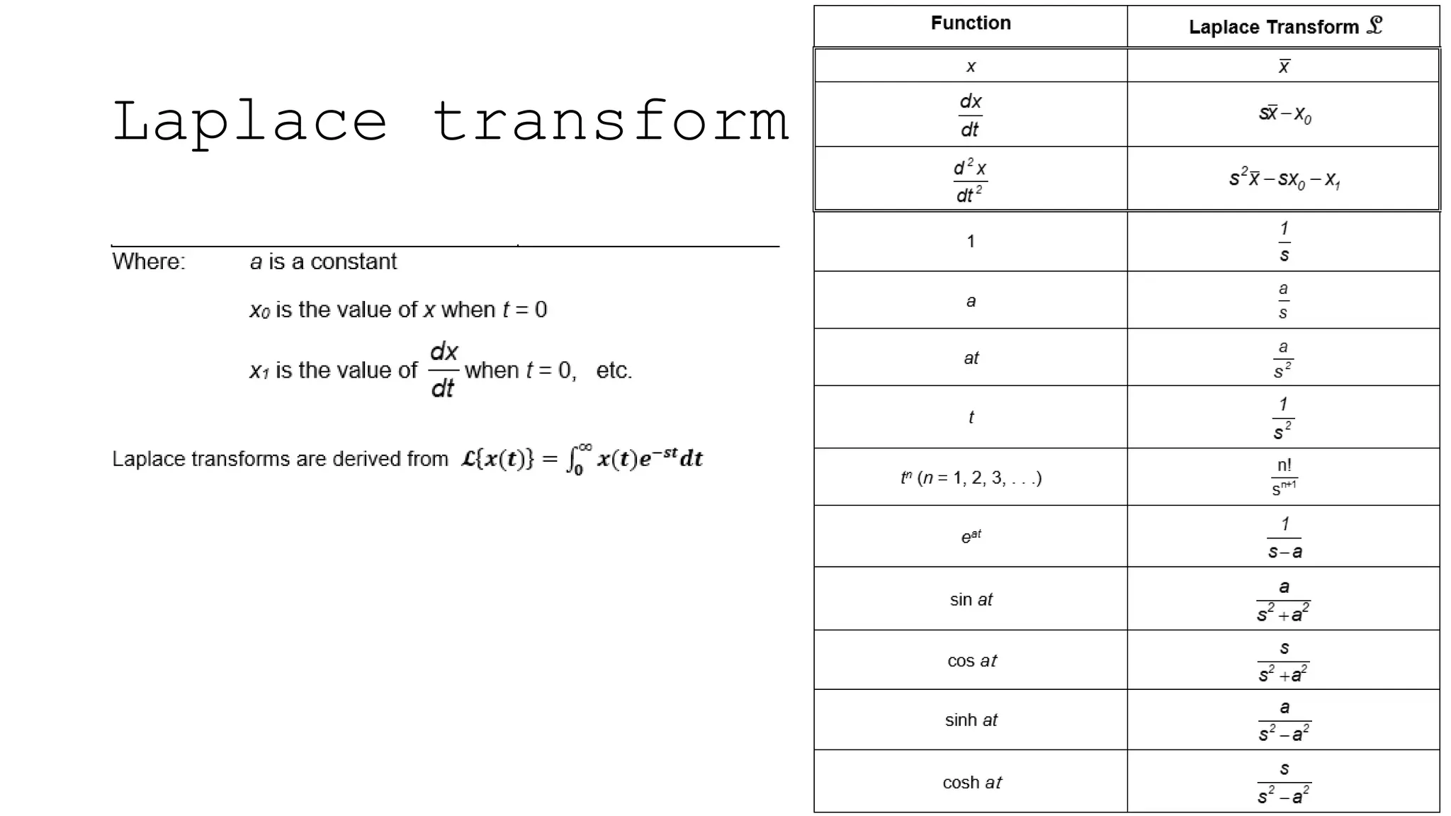
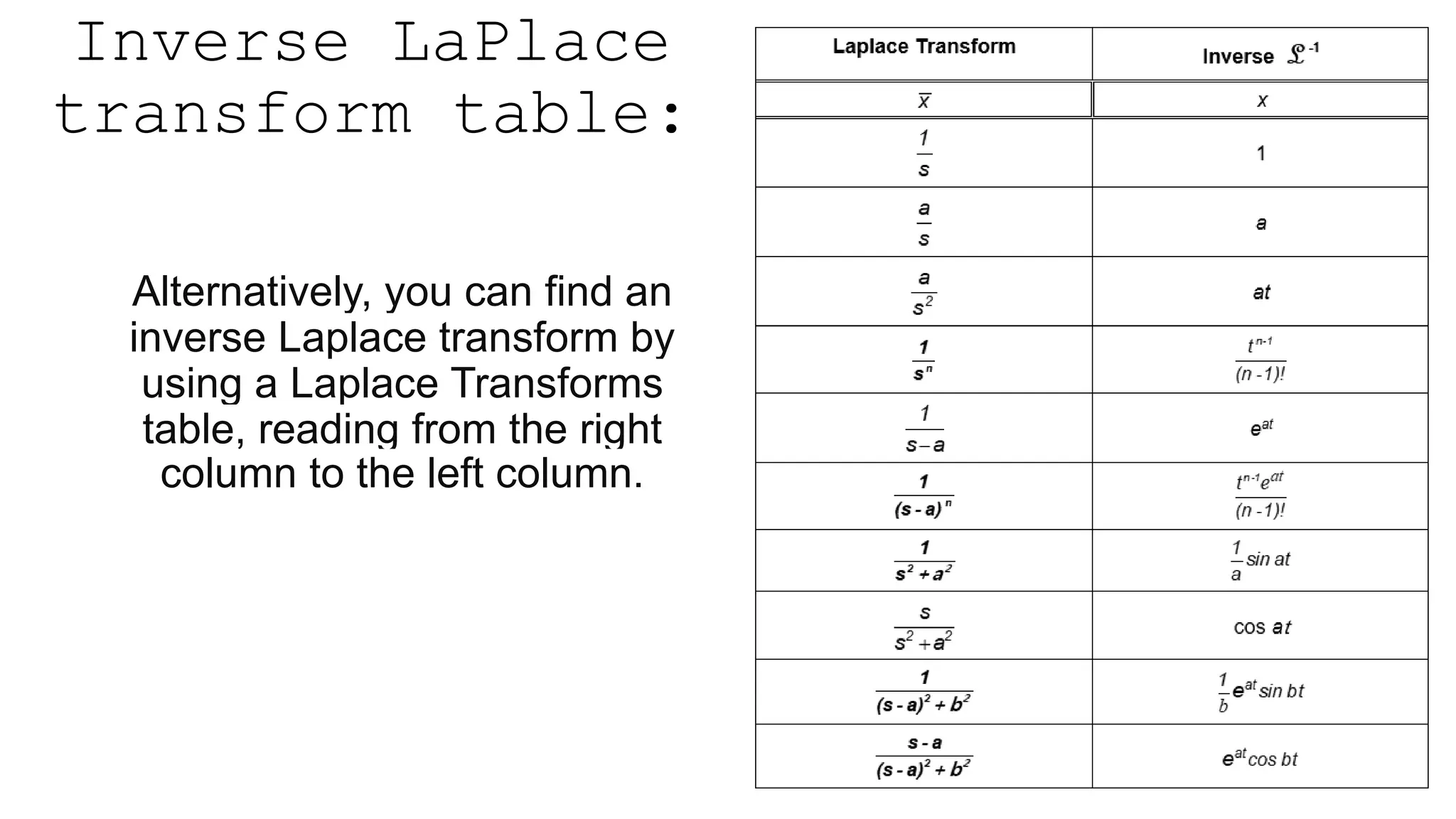
The document discusses key concepts in Laplace transforms including:
1) The Laplace transform is defined as an integral transform that transforms a function of time into a function of a complex variable, simplifying analysis of differential equations.
2) Important properties include the Laplace transforms of derivatives and integrals, which allow transforming differential equations into algebraic equations.
3) The existence theorem guarantees a unique solution to initial value problems under certain conditions on the function.
The document discusses the Laplace transform, which takes a function of time and transforms it into a function of complex frequency. This transformation converts differential equations into algebraic equations, simplifying solving problems involving systems. The Laplace transform has many applications in fields like engineering, physics, and astronomy by allowing analysis of linear time-invariant systems through properties like derivatives becoming multiplications in the frequency domain.
This document discusses applying the Laplace transform to modeling the vocal tract. It begins with an abstract discussing the Laplace transform and its properties. It then discusses a generalized acoustic tube model of the vocal tract that includes the oral cavity, nasal cavity, and main vocal tract. The model considers a branch section where the three branches meet. The document discusses obtaining the transfer function from this generalized model and using it to formulate a pole-zero type linear prediction algorithm. It will evaluate the prediction coefficients and reflection coefficients by analyzing voiced and nasal sounds.
The document discusses the Laplace transform and its applications. The Laplace transform maps functions defined in the time domain to functions defined in the complex frequency domain. It makes solving differential equations easier by converting calculus operations into algebra. Some key properties include: the Laplace transform of derivatives can be obtained algebraically instead of using calculus rules, and the transform allows shifting between time and complex frequency domains. Examples are provided to illustrate definitions, properties, and how to use Laplace transforms to solve initial value problems for ordinary differential equations.
The document discusses Laplace transforms, which convert functions of time into functions of frequency to make differential equations easier to solve. Laplace transforms are useful for solving complex differential equations by converting them into simpler polynomial equations. The document also outlines several applications of Laplace transforms in fields like control systems, signal processing, physics, and circuit analysis.
This document provides an overview of analog control systems and Laplace transforms. It introduces key concepts like Laplace transforms, common time domain inputs, transfer functions, and modeling electrical, mechanical and electromechanical systems using block diagrams and mathematical models. Examples are provided to illustrate Laplace transforms, transfer functions, and analyzing system response using poles, zeros and stability analysis.
The document presents information about Laplace transforms including:
- The definition and properties of the Laplace transform. It transforms differential equations into algebraic equations.
- Examples of applications in solving ordinary and partial differential equations, electrical circuits, and other fields.
- Limitations in that it can only be used to solve differential equations with known constants.
- Conclusion that the Laplace transform is a powerful mathematical tool used across many areas of science and engineering.
This document discusses the Laplace transformation, which converts a function into another function through mathematical manipulation. Specifically, it transforms a differential equation into an algebraic expression that can be easily solved. The document outlines the key topics that will be covered, including the definition of the Laplace transform, using tables of transforms to solve problems, inverse transforms, step functions, and using Laplace transforms to solve initial value problems, especially those involving step functions. It aims to illustrate how Laplace transforms simplify solving differential equations.
Using Laplace Transforms to Solve Differential EquationsGeorge Stevens
This document discusses using Laplace transforms to solve differential equations. It begins with an introduction to Laplace transforms and their inventor Pierre-Simon Laplace. The author then explains that Laplace transforms can be used to transform differential equations into simpler algebraic equations that are easier to solve. As an example, the document walks through using Laplace transforms to solve a first order differential equation. It concludes that Laplace transforms are an important mathematical tool for solving differential equations.
The document discusses the simplex algorithm for solving linear programming problems. It begins with an introduction and overview of the simplex algorithm. It then describes the key steps of the algorithm, which are: 1) converting the problem into slack format, 2) constructing the initial simplex tableau, 3) selecting the pivot column and calculating the theta ratio to determine the departing variable, 4) pivoting to create the next tableau. The document provides examples to illustrate these steps. It also briefly discusses cycling issues, software implementations, efficiency considerations and variants of the simplex algorithm.
The Laplace transform is an integral transform that converts a function of time (often a function that represents a signal) into a function of complex frequency. It has various applications in engineering for solving differential equations and analyzing linear systems. The key aspect is that it converts differential operators into algebraic operations, allowing differential equations to be solved as algebraic equations. This makes the equations much easier to manipulate and solve compared to the original differential form.
This document describes the method of multiple scales for extracting the slow time dependence of patterns near a bifurcation. The key aspects are:
1) Introducing scaled space and time coordinates (multiple scales) to capture slow modulations to the pattern, treating these as separate variables.
2) Expanding the solution as a power series in a small parameter near threshold.
3) Equating terms at each order in the expansion to derive amplitude equations for the slowly varying amplitudes, using solvability conditions to constrain the equations.
4) The solvability conditions arise because the linear operator has a null space, requiring the removal of components in this null space for finite solutions.
The document discusses the Laplace transform and its applications. Specifically:
- The Laplace transform was developed by mathematicians including Euler, Lagrange, and Laplace to solve differential equations.
- It transforms a function of time to a function of complex frequencies, allowing differential equations to be written as algebraic equations.
- For a function to have a Laplace transform, it must be at least piecewise continuous and bounded above by an exponential function.
- The Laplace transform can reduce the dimension of partial differential equations and is used in applications including semiconductor mobility, wireless networks, vehicle vibrations, and electromagnetic fields.
1) The document describes using the Laplace transform method to derive equations for receptor-ligand binding kinetics models.
2) The Laplace transform allows time-dependent differential equations to be solved using simple algebra by transforming them into another mathematical domain.
3) Four binding models are presented: ligand association, dissociation, unlabeled ligand pre-incubation and washout, and competition kinetics. The method is applied step-by-step to derive the analytic equations for each model.
1) The document describes using the Laplace transform method to derive equations for receptor-ligand binding kinetics models.
2) The Laplace transform allows time-dependent differential equations to be solved using simple algebra by transforming them into another mathematical domain.
3) Four binding models are used as examples: ligand association, dissociation, unlabeled ligand pre-incubation and washout, and competition kinetics. Through taking the Laplace transform, substituting terms, and taking the inverse transform, analytical solutions are obtained for each model.
This document discusses applications of Taylor series and partial differential equations. Taylor series can be used to represent complicated functions as infinite polynomials, making their properties easier to study. They also allow differential equations to be solved more easily. Some applications discussed include using Taylor series to evaluate definite integrals of functions without anti-derivatives, study the asymptotic behavior of electric fields, and solve partial differential equations like the heat equation. Taylor series provide a way to approximate functions with polynomials.
The document discusses techniques for calculating derivatives of functions, including:
- Using formulas and theorems to calculate derivatives more efficiently than using the definition of a derivative.
- Applying rules like the power rule, product rule, and quotient rule to take derivatives.
- Using derivatives to find equations of tangent lines and instantaneous rates of change.
The Laplace transform is a mathematical tool that is useful for solving differential equations. It was developed by Pierre-Simon Laplace in the late 18th century. The Laplace transform takes a function of time and transforms it into a function of complex quantities. This transformation allows differential equations to be converted into algebraic equations that are easier to solve. Some common applications of the Laplace transform include modeling problems in semiconductors, wireless networks, vibrations, and electromagnetic fields.
The Laplace transform is an integral transform that converts a function of time into a function of complex frequency. It is defined as the integral of the function multiplied by e-st from 0 to infinity. The Laplace transform is used to solve differential equations by converting them to algebraic equations. Some key properties of the Laplace transform include linearity, shifting theorems, differentiation and integration formulas, and methods for periodic and anti-periodic functions.
Laplace Transformation & Its ApplicationChandra Kundu
This document presents an overview of the Laplace transform and its applications. It begins with an introduction to Laplace transforms as a mathematical tool to convert differential equations into algebraic expressions. It then provides definitions and properties of both the Laplace transform and its inverse. Examples are given of how Laplace transforms can be used to solve ordinary and partial differential equations, as well as applications in electrical circuits and other fields. The document concludes by noting some limitations of the Laplace transform method and references additional resources.
The document provides an introduction to the Laplace transform and its applications in engineering analysis. It discusses key topics including:
- The history and development of the Laplace transform by mathematician Pierre-Simon Laplace.
- How the Laplace transform is used to transform a variable like time or position into a parameter to solve differential equations.
- Examples of using Laplace transform properties like linearity, shifting, and change of scale to calculate transforms of functions.
- How Laplace transforms can be used to solve ordinary and partial differential equations that model physical systems.
- Tables of common Laplace transforms to help with transforming functions.
The document provides an overview of the simplex algorithm for solving linear programming problems. It begins with an introduction and defines the standard format for representing linear programs. It then describes the key steps of the simplex algorithm, including setting up the initial simplex tableau, choosing the pivot column and pivot row, and pivoting to move to the next basic feasible solution. It notes that the algorithm terminates when an optimal solution is reached where all entries in the objective row are non-negative. The document also briefly discusses variants like the ellipsoid method and cycling issues addressed by Bland's rule.
This document outlines the contents and structure of a course on Mathematics-I. It covers topics such as ordinary differential equations, linear differential equations, functions of several variables, vector calculus, and Laplace transforms. It lists textbooks and references for the course. It provides an overview of the 12 lectures in the Laplace transforms unit, covering definitions, properties, and applications of the Laplace transform to solve differential equations.
This document discusses the inverse Laplace transform, which finds the original function given its Laplace transform. It defines the inverse Laplace transform and proves it is unique. The key points are:
1. The inverse Laplace transform of a function F(s) is the function f(t) whose Laplace transform is F(s).
2. The uniqueness theorem proves there is only one function f(t) that corresponds to a given F(s).
3. The inverse is only defined for t ≥ 0, as the Laplace transform only uses information from the positive t-axis.
Partial fraction decomposition for inverse laplace transformVishalsagar657
This document discusses partial fraction decomposition for inverse Laplace transforms. It begins with an introduction to partial fraction decomposition and why it is useful for integration. It then covers various cases for partial fraction decomposition of inverse Laplace transforms, including when the denominator is a quadratic with two real roots, a double root, or complex conjugate roots. It also covers the case when the denominator is a cubic with one real and two complex conjugate roots. The goal is to decompose the function into simpler forms that can be easily inverted using the Laplace transform table.
Similar to Laplace Transforms.pptxhhhhhhhhhhhhhhhhh (20)
Epcon is One of the World's leading Manufacturing Companies.EpconLP
Epcon is One of the World's leading Manufacturing Companies. With over 4000 installations worldwide, EPCON has been pioneering new techniques since 1977 that have become industry standards now. Founded in 1977, Epcon has grown from a one-man operation to a global leader in developing and manufacturing innovative air pollution control technology and industrial heating equipment.
ENVIRONMENT~ Renewable Energy Sources and their future prospects.tiwarimanvi3129
This presentation is for us to know that how our Environment need Attention for protection of our natural resources which are depleted day by day that's why we need to take time and shift our attention to renewable energy sources instead of non-renewable sources which are better and Eco-friendly for our environment. these renewable energy sources are so helpful for our planet and for every living organism which depends on environment.
Kinetic studies on malachite green dye adsorption from aqueous solutions by A...Open Access Research Paper
Water polluted by dyestuffs compounds is a global threat to health and the environment; accordingly, we prepared a green novel sorbent chemical and Physical system from an algae, chitosan and chitosan nanoparticle and impregnated with algae with chitosan nanocomposite for the sorption of Malachite green dye from water. The algae with chitosan nanocomposite by a simple method and used as a recyclable and effective adsorbent for the removal of malachite green dye from aqueous solutions. Algae, chitosan, chitosan nanoparticle and algae with chitosan nanocomposite were characterized using different physicochemical methods. The functional groups and chemical compounds found in algae, chitosan, chitosan algae, chitosan nanoparticle, and chitosan nanoparticle with algae were identified using FTIR, SEM, and TGADTA/DTG techniques. The optimal adsorption conditions, different dosages, pH and Temperature the amount of algae with chitosan nanocomposite were determined. At optimized conditions and the batch equilibrium studies more than 99% of the dye was removed. The adsorption process data matched well kinetics showed that the reaction order for dye varied with pseudo-first order and pseudo-second order. Furthermore, the maximum adsorption capacity of the algae with chitosan nanocomposite toward malachite green dye reached as high as 15.5mg/g, respectively. Finally, multiple times reusing of algae with chitosan nanocomposite and removing dye from a real wastewater has made it a promising and attractive option for further practical applications.
Presented by The Global Peatlands Assessment: Mapping, Policy, and Action at GLF Peatlands 2024 - The Global Peatlands Assessment: Mapping, Policy, and Action
Evolving Lifecycles with High Resolution Site Characterization (HRSC) and 3-D...Joshua Orris
The incorporation of a 3DCSM and completion of HRSC provided a tool for enhanced, data-driven, decisions to support a change in remediation closure strategies. Currently, an approved pilot study has been obtained to shut-down the remediation systems (ISCO, P&T) and conduct a hydraulic study under non-pumping conditions. A separate micro-biological bench scale treatability study was competed that yielded positive results for an emerging innovative technology. As a result, a field pilot study has commenced with results expected in nine-twelve months. With the results of the hydraulic study, field pilot studies and an updated risk assessment leading site monitoring optimization cost lifecycle savings upwards of $15MM towards an alternatively evolved best available technology remediation closure strategy.
Improving the viability of probiotics by encapsulation methods for developmen...Open Access Research Paper
The popularity of functional foods among scientists and common people has been increasing day by day. Awareness and modernization make the consumer think better regarding food and nutrition. Now a day’s individual knows very well about the relation between food consumption and disease prevalence. Humans have a diversity of microbes in the gut that together form the gut microflora. Probiotics are the health-promoting live microbial cells improve host health through gut and brain connection and fighting against harmful bacteria. Bifidobacterium and Lactobacillus are the two bacterial genera which are considered to be probiotic. These good bacteria are facing challenges of viability. There are so many factors such as sensitivity to heat, pH, acidity, osmotic effect, mechanical shear, chemical components, freezing and storage time as well which affects the viability of probiotics in the dairy food matrix as well as in the gut. Multiple efforts have been done in the past and ongoing in present for these beneficial microbial population stability until their destination in the gut. One of a useful technique known as microencapsulation makes the probiotic effective in the diversified conditions and maintain these microbe’s community to the optimum level for achieving targeted benefits. Dairy products are found to be an ideal vehicle for probiotic incorporation. It has been seen that the encapsulated microbial cells show higher viability than the free cells in different processing and storage conditions as well as against bile salts in the gut. They make the food functional when incorporated, without affecting the product sensory characteristics.
Optimizing Post Remediation Groundwater Performance with Enhanced Microbiolog...Joshua Orris
Results of geophysics and pneumatic injection pilot tests during 2003 – 2007 yielded significant positive results for injection delivery design and contaminant mass treatment, resulting in permanent shut-down of an existing groundwater Pump & Treat system.
Accessible source areas were subsequently removed (2011) by soil excavation and treated with the placement of Emulsified Vegetable Oil EVO and zero-valent iron ZVI to accelerate treatment of impacted groundwater in overburden and weathered fractured bedrock. Post pilot test and post remediation groundwater monitoring has included analyses of CVOCs, organic fatty acids, dissolved gases and QuantArray® -Chlor to quantify key microorganisms (e.g., Dehalococcoides, Dehalobacter, etc.) and functional genes (e.g., vinyl chloride reductase, methane monooxygenase, etc.) to assess potential for reductive dechlorination and aerobic cometabolism of CVOCs.
In 2022, the first commercial application of MetaArray™ was performed at the site. MetaArray™ utilizes statistical analysis, such as principal component analysis and multivariate analysis to provide evidence that reductive dechlorination is active or even that it is slowing. This creates actionable data allowing users to save money by making important site management decisions earlier.
The results of the MetaArray™ analysis’ support vector machine (SVM) identified groundwater monitoring wells with a 80% confidence that were characterized as either Limited for Reductive Decholorination or had a High Reductive Reduction Dechlorination potential. The results of MetaArray™ will be used to further optimize the site’s post remediation monitoring program for monitored natural attenuation.
Climate Change All over the World .pptxsairaanwer024
Climate change refers to significant and lasting changes in the average weather patterns over periods ranging from decades to millions of years. It encompasses both global warming driven by human emissions of greenhouse gases and the resulting large-scale shifts in weather patterns. While climate change is a natural phenomenon, human activities, particularly since the Industrial Revolution, have accelerated its pace and intensity
Microbial characterisation and identification, and potability of River Kuywa ...Open Access Research Paper
Water contamination is one of the major causes of water borne diseases worldwide. In Kenya, approximately 43% of people lack access to potable water due to human contamination. River Kuywa water is currently experiencing contamination due to human activities. Its water is widely used for domestic, agricultural, industrial and recreational purposes. This study aimed at characterizing bacteria and fungi in river Kuywa water. Water samples were randomly collected from four sites of the river: site A (Matisi), site B (Ngwelo), site C (Nzoia water pump) and site D (Chalicha), during the dry season (January-March 2018) and wet season (April-July 2018) and were transported to Maseno University Microbiology and plant pathology laboratory for analysis. The characterization and identification of bacteria and fungi were carried out using standard microbiological techniques. Nine bacterial genera and three fungi were identified from Kuywa river water. Clostridium spp., Staphylococcus spp., Enterobacter spp., Streptococcus spp., E. coli, Klebsiella spp., Shigella spp., Proteus spp. and Salmonella spp. Fungi were Fusarium oxysporum, Aspergillus flavus complex and Penicillium species. Wet season recorded highest bacterial and fungal counts (6.61-7.66 and 3.83-6.75cfu/ml) respectively. The results indicated that the river Kuywa water is polluted and therefore unsafe for human consumption before treatment. It is therefore recommended that the communities to ensure that they boil water especially for drinking.
4. Step 1 – Laplace transform the
whole differential equation:
Use the transform table to
convert everything in the
differential equation into
LaPlace form. Some examples
are:
initial values – i.e. Replace
x0 and x1 with values (often 0)
Step 2 – Insert initial
values:
5. Step 3 -Rearrange to make the
subject of the equation
Factorise with outside a bracket on LHS
initially, then rearrange to make
the subject of the equation. This put all s on
the RHS.
Make RHS a single fraction. If required
multiply RHS by the Step function 1/s
Factorise the denominator of the resulting
fraction (this will reveal the poles).
6. Step 4 -Partial Fractions –
Split the fraction and find
Residues values A, B, etc.
Several types of factor in the denominator are shown below. Rewrite these as shown, then find A, B,
C, etc. This can also be done in MATLAB using the residue function.
Step 5 - Inverse Laplace Transform of the whole
equation = ANSWER!
7. Why use LaPlace transforms?
The Laplace transform is a method used to solve differential equations
and model engineering systems. It helps derive both the
complementary function (transient response) and the particular
integral (steady-state response). Initial or boundary conditions can be
applied to find a complete solution, though they are often set to zero
for simplicity.
Deriving over time?
8. Notation:
The Laplace variable, s, is a complex variable,
which replaces time, t, (time domain).
s consists of a real and imaginary part.
Where σ is the real part related to stability of
system
ω is the imaginary part related to frequency
Often only the steady state response is required so
we set σ = 0 and s = jω is used, where and ω is
the frequency (in rad/s).
X bar or X(s) - When the variable x is transformed
by a Laplace transform it is renamed x bar , or
X(s)