Simulation

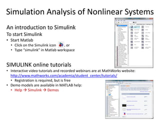
1. Simulation Analysis of Nonlinear Systems
An introduction to Simulink
To start Simulink
• Start Matlab
• Click on the Simulink icon , or
• Type “simulink” in Matlab workspace
SIMULINK online tutorials
• Interactive video tutorials and recorded webinars are at MathWorks website:
http://www.mathworks.com/academia/student_center/tutorials/
• Registration is required, but is free
• Demo models are available in MATLAB help:
• Help  Simulink  Demos

2. Example-1:
• Start Simulink
• Select File  New  Model (to open a new model window)
• Or, click on the ‘New Model’ icon
• Drag and drop blocks from the Library Browser in the new model window
• Connect the blocks appropriately
• Double-click blocks and set their parameters
• Select simulation solver and set parameters
• Simulation > Configuration Parameters…
• Start simulation and see results on scope
• Click ‘Start Simulation’ icon or press ‘Ctrl+T’
• Double-click on scope to see plots
Modeling with Simulink…

3. Modeling Nonlinear Systems
Example-2:
• Block diagram of a nonlinear system
• Equivalent Simulink model of the system
0.707
1
𝑠
𝑠+1
𝑠2+4𝑠+3
+
-
0.4
0.4
v=u+u3/6
+ -+ -
v u

4. Specifying Simulation Algorithm and
Solver Parameters
Example-2 continued:
Click on the “Simulation” tab
• In the “Configuration Parameters” window
specify
• Start and stop times
• Solver algorithm and options
• Variable or fixed step
• Ode45 (Dormand-Prince)
• Ode25s (stiff/NDF)
• Simulation accuracy
• Absolute and relative tolerance
• Minimum and maximum step size
• Warning and error messages

5. Simulating Nonlinear Systems
Example-2 continued
• Create subsystem
• Highlight system blocks
• Select: Edit > Create Subsystem, or press ‘Ctrl+G’
• Add ‘Signal Generator’ and ‘Scope’ (double-axis)
• Add a ‘To Workspace’ block to export signals to Matlab workspace
• The exported vector is named ‘simout’ (can be re-named)
• Start simulation () and observe results on scope
• You can also start simulation using sim() function
• [t,x,y]=sim(model_name,tf,options)
where options can be set as:
options=simset(property1,parameter1,property2,parameter2,…)

6. Modeling Hybrid Systems
Example-3:
• Block diagram of a hybrid (continuous + discrete) system
• Equivalent Simulink model of the system
G(s)D(z)
+
-
ZOH ZOH
R
T T T
Y(z)
T=0.2 
T=1 

7. Nonlinear Elements Modeling
• Modeling piecewise linear nonlinearities
– The one-dimensional “Look-up Table” block can be used
to represent piecewise-linear nonlinearities
– Other smooth nonlinearities can also be represented
• For example: y=tanh(x)
– Also “2-D Look-up Table” and “n-D Look-up Table” blocks
• User-defined functions
– “Fcn” block can define mathematical operations
– “Matlab Fcn” block embeds Matlab functions in Simulink
– “S-Function” is to embed “C” programs in Simulink

8. Linearization of nonlinear systems at an equilibrium point
Equilibrium point of a system
• Consider the system:
𝑥 = 𝑓 𝑥, 𝑢, 𝑡
𝑦 = ℎ 𝑥, 𝑢, 𝑡
where
𝑥 =
𝑥1
⋮
𝑥 𝑛
, 𝑢 =
𝑢1
⋮
𝑢 𝑚
, 𝑦 =
𝑦1
⋮
𝑦𝑝
, 𝑓 𝑥, 𝑢, 𝑡 =
𝑓1 𝑥1 … 𝑥 𝑛, 𝑢1 … 𝑢 𝑚, 𝑡
⋮
𝑓𝑛 𝑥1 … 𝑥 𝑛, 𝑢1 … 𝑢 𝑚, 𝑡
, and ℎ 𝑥, 𝑢, 𝑡 =
ℎ1 𝑥1 … 𝑥 𝑛, 𝑢1 … 𝑢 𝑚, 𝑡
⋮
ℎ 𝑝 𝑥1 … 𝑥 𝑛, 𝑢1 … 𝑢 𝑚, 𝑡
• An equilibrium-point is a point (𝑥 𝑒, 𝑢 𝑒) where 𝑥 = 0
• To find the equilibrium-points / operating-points (OP) of a system:
– Solve 𝑓 𝑥, 𝑢, 𝑡 = 0 for (𝑥, 𝑢)
In Matlab use the command ‘trim()’
Syntax: [x,u,y,z]=trim(model_name,x0,u0)
• x0,u0 are the initial guess
• x,u,y are the returned operating points
• z is the returned value of dx/dt at the estimated OP
Linearization of Nonlinear Models

9. Linearizing system model at an OP (𝑥 𝑒, 𝑢 𝑒)
• Expand 𝑓 𝑥, 𝑢, 𝑡 and ℎ 𝑥, 𝑢, 𝑡 about (𝑥 𝑒, 𝑢 𝑒)
‒ Use Taylor series expansion
‒ For time-invariant systems, t is not considered
𝑓 𝑥, 𝑢 = 𝑓 𝑥 𝑒, 𝑢 𝑒
0
+
𝜕𝑓
𝜕𝑥 𝑥=𝑥 𝑒
𝑢=𝑢 𝑒
𝑥 − 𝑥 𝑒 +
𝜕𝑓
𝜕𝑢 𝑥=𝑥 𝑒
𝑢=𝑢 𝑒
𝑢 − 𝑢 𝑒 + …
ℎ.𝑜.𝑡.
ℎ 𝑥, 𝑢 = ℎ 𝑥 𝑒, 𝑢 𝑒
0
+
𝜕ℎ
𝜕𝑥 𝑥=𝑥 𝑒
𝑢=𝑢 𝑒
𝑥 − 𝑥 𝑒 +
𝜕ℎ
𝜕𝑢 𝑥=𝑥 𝑒
𝑢=𝑢 𝑒
𝑢 − 𝑢 𝑒 + …
ℎ.𝑜.𝑡.
Let 𝑥 = 𝑥 − 𝑥 𝑒, 𝑢 = 𝑢 − 𝑢 𝑒, and 𝑥 = 𝑥 − 𝑥 𝑒
0
. Then, neglecting the h.o.t.’s, we get:
𝑥 =
𝜕𝑓
𝜕𝑥 𝑥=𝑥 𝑒
𝑢=𝑢 𝑒
𝐴
𝑥 +
𝜕𝑓
𝜕𝑢 𝑥=𝑥 𝑒
𝑢=𝑢 𝑒
𝐵
𝑢
𝑦 =
𝜕ℎ
𝜕𝑥 𝑥=𝑥 𝑒
𝑢=𝑢 𝑒
𝐶
𝑥 +
𝜕ℎ
𝜕𝑢 𝑥=𝑥 𝑒
𝑢=𝑢 𝑒
𝐷
𝑢

𝑥 = 𝐴 𝑥 + 𝐵 𝑢
𝑦 = 𝐶 𝑥 + 𝐷 𝑢
• In MATLAB, use the command ‘linmod()’
Linearization of Nonlinear Systems

10. Linear Approximation with Matlab/Simulink
Example
Consider the nonlinear system shown (chapter 4, example 1)
How can we find the transfer function of this system?
• A transfer function exists only for LTI systems, so we must find a linear
approximation of this model

11. Given a model in Simulink
• Use Matlab commands trim and linmod to find the operating point (OP) and
linearize the system model at that OP
• The linearized model can then be manipulated and analyzed in MATLAB
MATLAB code:
[xe,ue,ye,dxe]=trim('lect7',[],1);
[A,B,C,D]=linmod('lect7',xe,ue);
sys=ss(A,B,C,D);
G=tf(sys);
stepplot(G);
System Linearization of Simulink Models

12. • From the step response, it
appears that the system is
stable
• This could also be verified
using isstable() command or by
checking if the real parts of all
its eigenvalues are negative.
>> isstable(sys)
ans =
1
>> eig(sys)
ans =
-1.8535 + 0.8329i
-1.8535 - 0.8329i
-1.0000
System Linearization …

13. Example (same as example 3):
• Block diagram of the system
• Add other blocks for input and output collection
Linear Identification of Nonlinear Systems
G(s)D(z)
+
-
ZOH ZOH
R
T T T
Y(z)
Subsystem

14. Linear Identification of Nonlinear Systems
Example continued
• Simulate system with a ‘sufficiently rich’ input
• Export sampled I/O data to Matlab workspace
• Use ‘To Workspace’ block and set its sample-time, T=0.01
• In Matlab, from simout, construct uk and yk
• Use ‘ident’ to find a linear model of the system
• Verify the accuracy of the approximate linear model
Identified linear model:
𝐺 𝑠 ≅
0.4
𝑠2+3.707𝑠+3.121
Verify linear model accuracy: 0 1 2 3 4 5 6 7 8 9 10
-0.03
-0.02
-0.01
0
0.01
0.02
0.03
0.04
0.05
tk=simout(:,1);
uk=simout(:,2);
yk=simout(:,3);
% Run ident and find
% System model arx221
G221=tf(arx221);
Ghz=G221(1);
Ghs=d2c(Ghz)
yhk=lsim(Ghs,uk,tk);
plot(tk,yk,'r'), hold on,
plot(tk,yhk,'bo'); hold off,