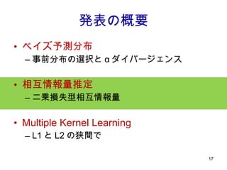
Mutual Information Commonstrategy : Find W which makes as independent as possible. Mutual Information is a good independence measure. are mutually independent. ⇔ : joint distribution of : marginal distribution of
20.
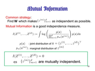
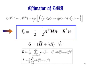
Our Proposal Squared-lossMutual Information (SMI) are mutually independent. ⇔ We propose a non-parametric estimator of I s thanks to squared loss, analytic solution is available Gradient of I s w.r.t. W is also analytically available gradient descent method for ICA and Dim. Reduction.
21.
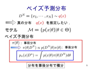
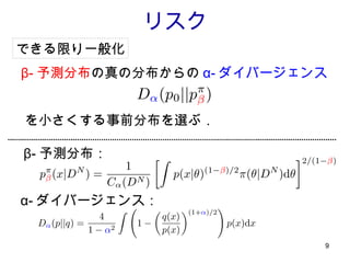
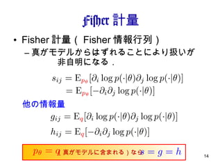
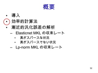
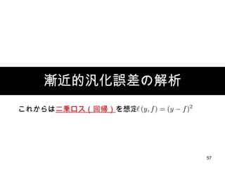
Estimation Method Estimatethe density ratio : (Legendre-Fenchel convex duality [Nguyen et al. 08] ) Define , then we can write where sup is taken over all measurable functions . the optimal function is the density ratio
22.
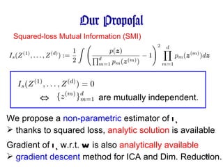
The problem isreduced to solving Empirical Approximation The objective function is empirically approximated as V-statistics (Decoupling) Assume we have n samples:
23.
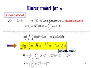
Linear model for g Linear model is basis function, e.g., Gaussian kernel penalty term
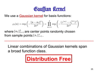
Gaussian Kernel Weuse a Gaussian kernel for basis functions: where are center points randomly chosen from sample points: . Linear combinations of Gaussian kernels span a broad function class. Distribution Free
26.
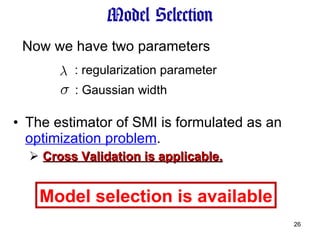
Model Selection Theestimator of SMI is formulated as an optimization problem . Cross Validation is applicable. Model selection is available Now we have two parameters : regularization parameter : Gaussian width
27.
Asymptotic Analysis Regularizationparameter : Theorem : Complexity of the model ( large:complex, small:simple ) Theorem Nonarametric Parametric : matrices like Fisher Information matrix (bracketing entropy condition)
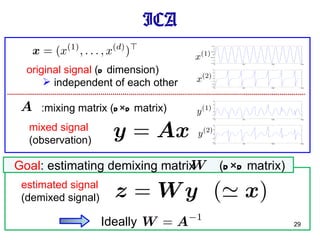
ICA mixed signal(observation) original signal ( d dimension) independent of each other estimated signal (demixed signal) :mixing matrix ( d × d matrix) Goal : estimating demixing matrix ( d × d matrix) Ideally
30.
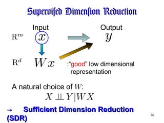
Supervised Dimension ReductionInput Output :“ good ” low dimensional representation -> Sufficient Dimension Reduction (SDR) A natural choice of W :
31.
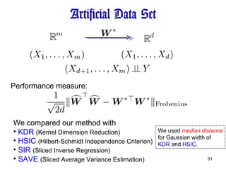
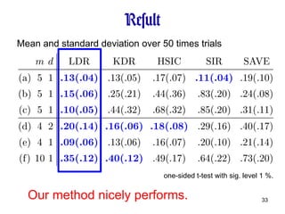
Artificial Data SetWe compared our method with KDR (Kernel Dimension Reduction) HSIC (Hilbert-Schmidt Independence Criterion) SIR (Sliced Inverse Regression) SAVE (Sliced Average Variance Estimation) Performance measure: We used median distance for Gaussian width of KDR and HSIC .
Result one-sided t-testwith sig. level 1 %. Mean and standard deviation over 50 times trials Our method nicely performs.
34.
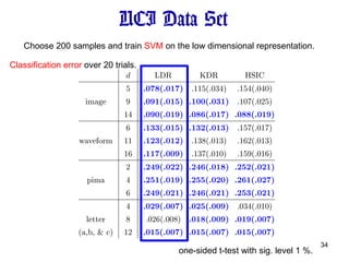
UCI Data Setone-sided t-test with sig. level 1 %. Choose 200 samples and train SVM on the low dimensional representation. Classification error over 20 trials.
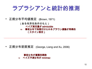
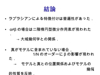
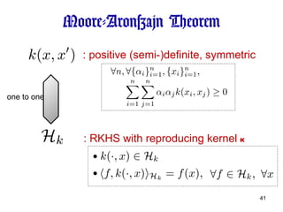
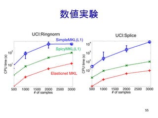
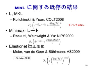
Sparse Learning :n samples : Convex loss ( hinge, square, logistic ) L 1 -regularization-> sparse Lasso Group Lasso I : subset of indices [Yuan&Lin:JRSS2006] [Tibshirani :JRSS1996]
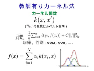
Reproducing Kernel HilbertSpace (RKHS) : Hilbert space of real valued functions : map to the Hilbert space such that Reproducing kernel Representer theorem
41.
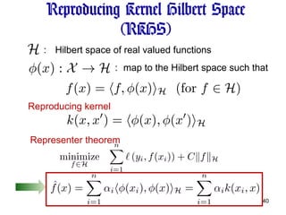
Moore-Aronszajn Theorem :positive (semi-)definite, symmetric : RKHS with reproducing kernel k one to one


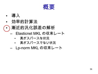
![結果 : を事前分布としたときの β- ベイズ予測分布 漸近的なリスクの差 [Suzuki&Komaki,2010] 二階微分作用素 ← 補正項 (α=β で 0) A 優調和関数であれば良い α=β の時,ラプラシアンによる特徴付けが現われる A に付随した拡散過程 が存在](https://image.slidesharecdn.com/jokyokai-110425221600-phpapp02/85/Jokyokai-10-320.jpg)

![Estimation Method Estimate the density ratio : (Legendre-Fenchel convex duality [Nguyen et al. 08] ) Define , then we can write where sup is taken over all measurable functions . the optimal function is the density ratio](https://image.slidesharecdn.com/jokyokai-110425221600-phpapp02/85/Jokyokai-21-320.jpg)

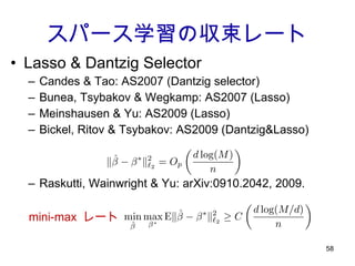
![Applications ICA (Independent Component Analysis) [Suzuki&Sugiyama, 2011] SDR (Sufficient Dimension Reduction) [Suzuki&Sugiyama, 2010] Independence Test [Sugiyama&Suzuki, 2011] Causal Inference [Yamada&Sugiyama, 2010]](https://image.slidesharecdn.com/jokyokai-110425221600-phpapp02/85/Jokyokai-28-320.jpg)
![Sparse Learning : n samples : Convex loss ( hinge, square, logistic ) L 1 -regularization-> sparse Lasso Group Lasso I : subset of indices [Yuan&Lin:JRSS2006] [Tibshirani :JRSS1996]](https://image.slidesharecdn.com/jokyokai-110425221600-phpapp02/85/Jokyokai-38-320.jpg)
![MKL: Multiple Kernel Learning : M 個のカーネル関数 : カーネル関数 k m に付随した RKHS [ Lanckriet et al. 2004 ] L1 正則化: スパース Gourp Lasso の無限次元への拡張 [Bach, Lanchriet, Jordan:ICML 2004 ]](https://image.slidesharecdn.com/jokyokai-110425221600-phpapp02/85/Jokyokai-43-320.jpg)
![カーネル重みとの関係 [Micchelli & Pontil: JMLR2005] 目的関数をカーネル関数の凸結合の中で最小化 : given k は k m らの凸結合 Young の不等式](https://image.slidesharecdn.com/jokyokai-110425221600-phpapp02/85/Jokyokai-44-320.jpg)
![L 1 と L 2 の橋渡し Elasticnet MKL Lp-norm MKL (1≦p≦2) [Marius et al.: NIPS2009] [Shawe-Taylor: NIPS workshop 2008, Tomioka & Suzuki: NIPS workshop 2009] cf. elastic-net: [Zou & Hastie: JRSS, 2005]](https://image.slidesharecdn.com/jokyokai-110425221600-phpapp02/85/Jokyokai-47-320.jpg)
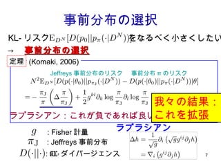
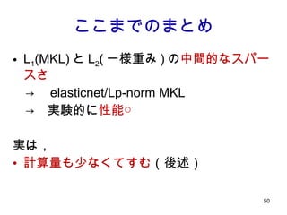
![Best Medium density dense [Tomioka & Suzuki: NIPS 2009 Workshop ] Elasticnet MKL: caltech 101 dataset L1 L2 中間的なスパースさが良い](https://image.slidesharecdn.com/jokyokai-110425221600-phpapp02/85/Jokyokai-48-320.jpg)
![[Cortes, Mohri, and Rostamizadeh: UAI 2009] MKL (sparse) 一様重み (dense) 中間 (p=4/3) Lp-norm MKL # of features](https://image.slidesharecdn.com/jokyokai-110425221600-phpapp02/85/Jokyokai-49-320.jpg)


![[DL輪読会]Neural Ordinary Differential Equations](https://cdn.slidesharecdn.com/ss_thumbnails/nnasode1-190111001755-thumbnail.jpg?width=640&height=640&fit=bounds)
![[DL輪読会]ICLR2020の分布外検知速報](https://cdn.slidesharecdn.com/ss_thumbnails/iclr2020ood-190927011524-thumbnail.jpg?width=640&height=640&fit=bounds)


![[DL輪読会]Meta Reinforcement Learning](https://cdn.slidesharecdn.com/ss_thumbnails/metarl-190201005548-thumbnail.jpg?width=640&height=640&fit=bounds)


![Infinite SVM [改] - ICML 2011 読み会](https://cdn.slidesharecdn.com/ss_thumbnails/isvm-icml11a-110719050617-phpapp02-thumbnail.jpg?width=640&height=640&fit=bounds)

![[ICLR2021 (spotlight)] Benefit of deep learning with non-convex noisy gradien...](https://cdn.slidesharecdn.com/ss_thumbnails/iclr2021-210331133549-thumbnail.jpg?width=640&height=640&fit=bounds)
![[NeurIPS2020 (spotlight)] Generalization bound of globally optimal non convex...](https://cdn.slidesharecdn.com/ss_thumbnails/neurips2020spotlight-210331133014-thumbnail.jpg?width=640&height=640&fit=bounds)