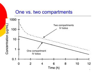
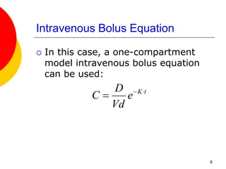
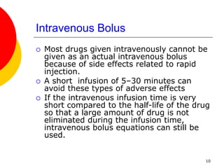
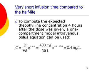
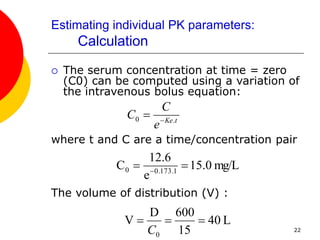
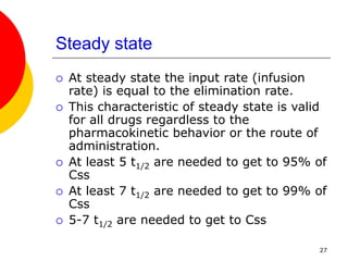
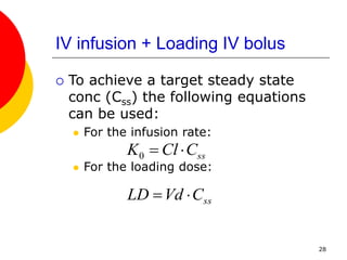
1
Clinical pharmacokinetic
equations and calculations
Mohammad Issa Saleh
2
One vs. two compartments
3
One vs. two compartments
Two compartments
IV bolus
One compartment
IV bolus
4
One vs. two compartments
 In many cases, the drug distributes
from the blood into the tissues
quickly, and a pseudoequilibrium of
drug movement between blood and
tissues is established rapidly. When
this occurs, a one-compartment
model can be used to describe the
serum concentrations of a drug.
5
One vs. two compartments
 In some clinical situations, it is
possible to use a one-compartment
model to compute doses for a drug
even if drug distribution takes time
to complete. In this case, drug
serum concentrations are not
obtained in a patient until after the
distribution phase is over.
6
One-compartment model equations
 IV bolus
 IV infusion
 Extravascular
7
Intravenous Bolus Equation
 When a drug is given as an
intravenous bolus and the drug
distributes from the blood into the
tissues quickly, the serum
concentrations often decline in a
straight line when plotted on
semilogarithmic axes (Figure next
slide).
8
Intravenous Bolus Equation
 In this case, a one-compartment
model intravenous bolus equation
can be used:
t
K
e
Vd
D
C 


9
Intravenous Bolus Equation
t
K
e
Vd
D
C 


10
Intravenous Bolus
 Most drugs given intravenously cannot be
given as an actual intravenous bolus
because of side effects related to rapid
injection.
 A short infusion of 5–30 minutes can
avoid these types of adverse effects
 If the intravenous infusion time is very
short compared to the half-life of the drug
so that a large amount of drug is not
eliminated during the infusion time,
intravenous bolus equations can still be
used.
11
Very short infusion time compared to
the half-life
 For example, a patient is given a
theophylline loading dose of 400 mg
intravenously over 20 minutes.
Because the patient received
theophylline during previous
hospitalizations, it is known that the
volume of distribution is 30 L, the
elimination rate constant equals
0.116 h−1, and the half-life (t1/2) is
6 hours (t1/2 = 0.693/ke =
0.693/0.115 h−1 = 6 h).
12
Very short infusion time compared to
the half-life
 To compute the expected
theophylline concentration 4 hours
after the dose was given, a one-
compartment model intravenous
bolus equation can be used:
mg/L
8.4
e
L
30
mg
400
e
Vd
D
C 4
0.115
t
K


 



13
Slow infusion and/or distribution
 If drug distribution is not rapid, it is
still possible to use a one
compartment model intravenous
bolus equation if the duration of the
distribution phase and infusion time
is small compared to the half-life of
the drug and only a small amount of
drug is eliminated during the
infusion and distribution phases
14
Slow infusion and/or distribution
 For instance, vancomycin must be infused
slowly over 1 hour in order to avoid
hypotension and red flushing around the
head and neck areas. Additionally,
vancomycin distributes slowly to tissues
with a 1/2–1 hour distribution phase.
Because the half-life of vancomycin in
patients with normal renal function is
approximately 8 hours, a one
compartment model intravenous bolus
equation can be used to compute
concentrations in the postinfusion,
postdistribution phase without a large
amount of error.
15
Slow infusion and/or distribution
 As an example of this approach (previous slide), a
patient is given an intravenous dose of
vancomycin 1000 mg. Since the patient has
received this drug before, it is known that the
volume of distribution equals 50 L, the elimination
rate constant is 0.077 h−1, and the half-life
equals 9 h (t1/2 = 0.693/ke = 0.693/0.077 h−1
= 9 h).
 To calculate the expected vancomycin
concentration 12 hours after the dose was given,
a one compartment model intravenous bolus
equation can be used:
mg/L
7.9
e
L
50
mg
1000
e
Vd
D
C 12
0.077
t
K


 



16
Estimating individual Pharmacokinetic
parameters: IV bolus
1. Plotting
2. Simple fitting (will not be
discussed)
3. Calculation
17
Estimating individual PK parameters:
plotting
 For example, a patient was given an
intravenous loading dose of phenobarbital
600 mg over a period of about an hour.
One day and four days after the dose was
administered phenobarbital serum
concentrations were 12.6 mg/L and 7.5
mg/L, respectively.
 By plotting the serum concentration/time
data on semilogarithmic axes, the time it
takes for serum concentrations to
decrease by one-half can be determined
and is equal to 4 days.
18
Estimating individual PK parameters:
plotting
19
Estimating individual PK parameters:
plotting
 The elimination rate constant can be
computed using the following
relationship:
 The extrapolated concentration at
time = 0 (C0 = 15 mg/L in this
case) can be used to calculate the
volume of distribution:
1
-
2
/
1
day
173
.
0
4
0.693
t
0.693



Ke
L
40
15
600
D
V
0



C
20
Estimating individual PK parameters:
Calculation
 Alternatively, these parameters could be
obtained by calculation without plotting
the concentrations.
 The elimination rate constant can be
computed using the following equation:
where t1 and C1 are the first
time/concentration pair and t2 and C2 are
the second time/concentration pair
day
0.173
4
-
1
ln(7.5)
-
ln(12.6)
-
t
-
t
)
ln(C
-
)
ln(C
-
Ke 1
-
2
1
2
1

















21
Estimating individual PK parameters:
Calculation
 The elimination rate constant can be
converted into the half-life using the
following equation:
days
4
173
.
0
0.693
0.693
t 2
/
1 


Ke
22
Estimating individual PK parameters:
Calculation
 The serum concentration at time = zero
(C0) can be computed using a variation of
the intravenous bolus equation:
where t and C are a time/concentration pair
The volume of distribution (V) :
t
Ke
e
C
C .
0 

mg/L
15.0
e
12.6
C 0.173.1
0 
 
L
40
15
600
D
V
0



C
23
Continuous intravenous infusion
(one-compartment model)
Dr Mohammad Issa
24
IV infusion
0
5
10
15
20
25
30
35
0 5 10 15 20 25 30 35 40
Time
Concentration
During infusion Post infusion
25
IV infusion: during infusion
0
5
10
15
20
25
30
35
0 5 10 15 20 25 30 35 40
Time
Concentration
where K0 is the infusion
rate, K is the elimination
rate constant, and Vd is
the volume of distribution
)
1
( e
Kt
o
K
K
X



)
1
( e
Kt
o
p
KVd
K
C



26
Steady state
0
5
10
15
20
25
30
35
0 5 10 15 20 25 30 35 40
Time
Concentration
≈ steady state
concentration (Css)
KVd
K
C
o
ss 
27
Steady state
 At steady state the input rate (infusion
rate) is equal to the elimination rate.
 This characteristic of steady state is valid
for all drugs regardless to the
pharmacokinetic behavior or the route of
administration.
 At least 5 t1/2 are needed to get to 95% of
Css
 At least 7 t1/2 are needed to get to 99% of
Css
 5-7 t1/2 are needed to get to Css
28
IV infusion + Loading IV bolus
 To achieve a target steady state
conc (Css) the following equations
can be used:
 For the infusion rate:
 For the loading dose:
ss
C
Cl
K 

0
ss
C
Vd
LD 

29
Concentration
Concentration
Concentration
Concentration
Half-lives
Half-lives
Half-lives
Half-lives
Case A
Infusion alone
(K0= Css∙Cl)
Case B
Infusion (K0= Css∙Cl)
loading bolus (LD= Css∙Vd)
Case D
Infusion (K0= Css∙Cl)
loading bolus (LD< Css∙Vd)
Case C
Infusion (K0= Css∙Cl)
loading bolus (LD > Css∙Vd)
Scenarios with different LD
30
Post infusion phase
0
5
10
15
20
25
30
35
0 5 10 15 20 25 30 35 40
Time
Concentration
During infusion Post infusion
Cend
(Concentration
at the end of
the infusion)
e
Kt
end
postinf C
C



)
1
( e
KT
o
end
KVd
K
C



t is the post infusion time
T is the infusion duration
31
Post infusion phase data
 Half-life and elimination rate
constant calculation
 Volume of distribution estimation
32
Elimination rate constant calculation
using post infusion data
 K can be estimated using post
infusion data by:
 Plotting log(Conc) vs. time
 From the slope estimate K:
303
.
2
k
Slope 

33
Volume of distribution calculation using
post infusion data
 If you reached steady state conc
(C* = CSS):
 where k is estimated as described in
the previous slide
ss
ss
C
K
K
Vd
Vd
K
K
C




 0
0
34
Volume of distribution calculation using
post infusion data
 If you did not reached steady state
(C* = CSS(1-e-kT)):
)
1
(
*
)
1
(
* 0
0 kT
kT
e
C
k
k
Vd
e
Vd
k
k
C 








35
Example 1
Following a two-hour infusion of 100
mg/hr plasma was collected and
analysed for drug concentration.
Calculate kel and V.
Time relative
to infusion
cessation
(hr)
1 3 7 10 16 22
Cp (mg/L) 12 9 8 5 3.9 1.7
36
Post infusion data
y = -0.0378x + 1.1144
R2
= 0.9664
0
0.2
0.4
0.6
0.8
1
1.2
0 5 10 15 20 25
Time (hr)
Log(Conc)
mg/L
Time is the time after stopping the infusion
37
Example 1
 From the slope, K is estimated to
be:
 From the intercept, C* is estimated
to be:
1/hr
0.087
0.0378
2.303
Slope
2.303
k 







mg/L
13
10
C*
1.1144
intercept
log(C*)
1.1144




38
Example 1
 Since we did not get to steady
state:
L
14.1
)
e
(1
(13)
(0.087)
100
Vd
)
e
(1
*
C
k
k
Vd
2
0.087*
kT
0









39
Example 2
 Estimate the volume of distribution
(22 L), elimination rate constant
(0.28 hr-1), half-life (2.5 hr), and
clearance (6.2 L/hr) from the data in
the following table obtained on
infusing a drug at the rate of 50
mg/hr for 16 hours.
Time
(hr)
0 2 4 6 10 12 15 16 18 20 24
Conc
(mg/L)
0 3.48 5.47 6.6 7.6 7.8 8 8 4.6 2.62 0.85
40
Example 2
41
Example 2
1. Calculating clearance:
It appears from the data that the
infusion has reached steady state:
(CP(t=15) = CP(t=16) = CSS)
L/hr
25
.
6
mg/L
8
mg/hr
50
0
0





SS
SS
C
K
Cl
Cl
K
C
42
Example 2
2. Calculating elimination rate constant
and half life:
From the post infusion data, K and t1/2 can
be estimated. The concentration in the
post infusion phase is described
according to:
where t1 is the time after stopping the
infusion. Plotting log(Cp) vs. t1 results
in the following:
1
303
.
2
)
log(
)
log(
1
t
K
C
C
e
C
C SS
P
t
K
SS
P 



 

43
Example 2
y = -0.1218x + 0.9047
R2
= 1
-0.2
0
0.2
0.4
0.6
0.8
1
0 1 2 3 4 5 6 7 8 9
Post infusion time (hr)
log(Conc)
(mg/L)
44
Example 2
K=-slope*2.303=0.28 hr-1
Half life = 0.693/K=0.693/0.28=
2.475 hr
3. Calculating volume of distribution:
L
3
.
22
hr
28
.
0
L/hr
25
.
6
1
-



K
Cl
VD
45
Example 3
 For prolonged surgical procedures,
succinylcholine is given by IV
infusion for sustained muscle
relaxation. A typical initial dose is 20
mg followed by continuous infusion
of 4 mg/min. the infusion must be
individualized because of variation in
the kinetics of metabolism of
suucinylcholine. Estimate the
elimination half-lives of
succinylcholine in patients requiring
0.4 mg/min and 4 mg/min,
respectively, to maintain 20 mg in the
body. (35 and 3.5 min)
46
Example 3
For the patient requiring 0.4 mg/min:
For the patient requiring 4 mg/min:
0
2
/
1
2
/
1
0
693
.
0
693
.
0 K
A
t
t
K
K
K
A SS
o
ss






min
65
.
34
4
.
0
)
693
.
0
)(
20
(
693
.
0
0
2
/
1 



K
A
t SS
min
465
.
3
4
)
693
.
0
)(
20
(
693
.
0
0
2
/
1 



K
A
t SS
47
Example 4
A drug is administered as a short
term infusion. The average
pharmacokinetic parameters for
this
drug are:
K = 0.40 hr-1
Vd = 28 L
This drug follows a one-
compartment body model.
48
Example 4
1) A 300 mg dose of this drug is given
as a short-term infusion over 30
minutes. What is the infusion rate?
What will be the plasma
concentration at the end of the
infusion?
2) How long will it take for the plasma
concentration to fall to 5.0 mg/L?
3) If another infusion is started 5.5
hours after the first infusion was
stopped, what will the plasma
concentration be just before the
second infusion?
49
Example 4
1) The infusion rate (K0) =
Dose/duration = 300 mg/0.5 hr =
600 mg/hr.
Plasma concentration at the end of
the infusion:
Infusion phase:
 
mg/L
71
.
9
)
1
(
L)
28
)(
hr
4
.
0
(
mg/hr
600
hr)
5
.
0
(
1
C
)
5
.
0
)(
4
.
0
(
1
-
0
P










e
t
C
e
V
K
K
P
t
K
D
50
Example 4
2) Post infusion phase:
The concentration will fall to 5.0 mg/L
1.66 hr after the infusion was
stopped.
hr
1.66
0.4
ln(5)
ln(9.71)
K
)
ln(C
-
infusion))
of
end
(at the
ln(C
t
t
K
-
infusion))
of
end
(at the
ln(C
)
ln(C
e
infusion)
of
end
(at the
C
C
P
P
2
2
P
P
t
k
P
P
2









 

51
Example 4
3) Post infusion phase (conc 5.5 hrs
after stopping the infusion):
mg/L
08
.
1
9.71)e
(
hr)
5.5
(t
C
e
infusion)
of
end
(at the
C
C
-.4)(5.5)
(-0
p
t
k
P
P
2




 

52

IV-Bolus-and-Infusion.ppt

  • 1.
    1 Clinical pharmacokinetic equations andcalculations Mohammad Issa Saleh
  • 2.
    2 One vs. twocompartments
  • 3.
    3 One vs. twocompartments Two compartments IV bolus One compartment IV bolus
  • 4.
    4 One vs. twocompartments  In many cases, the drug distributes from the blood into the tissues quickly, and a pseudoequilibrium of drug movement between blood and tissues is established rapidly. When this occurs, a one-compartment model can be used to describe the serum concentrations of a drug.
  • 5.
    5 One vs. twocompartments  In some clinical situations, it is possible to use a one-compartment model to compute doses for a drug even if drug distribution takes time to complete. In this case, drug serum concentrations are not obtained in a patient until after the distribution phase is over.
  • 6.
    6 One-compartment model equations IV bolus  IV infusion  Extravascular
  • 7.
    7 Intravenous Bolus Equation When a drug is given as an intravenous bolus and the drug distributes from the blood into the tissues quickly, the serum concentrations often decline in a straight line when plotted on semilogarithmic axes (Figure next slide).
  • 8.
    8 Intravenous Bolus Equation In this case, a one-compartment model intravenous bolus equation can be used: t K e Vd D C   
  • 9.
  • 10.
    10 Intravenous Bolus  Mostdrugs given intravenously cannot be given as an actual intravenous bolus because of side effects related to rapid injection.  A short infusion of 5–30 minutes can avoid these types of adverse effects  If the intravenous infusion time is very short compared to the half-life of the drug so that a large amount of drug is not eliminated during the infusion time, intravenous bolus equations can still be used.
  • 11.
    11 Very short infusiontime compared to the half-life  For example, a patient is given a theophylline loading dose of 400 mg intravenously over 20 minutes. Because the patient received theophylline during previous hospitalizations, it is known that the volume of distribution is 30 L, the elimination rate constant equals 0.116 h−1, and the half-life (t1/2) is 6 hours (t1/2 = 0.693/ke = 0.693/0.115 h−1 = 6 h).
  • 12.
    12 Very short infusiontime compared to the half-life  To compute the expected theophylline concentration 4 hours after the dose was given, a one- compartment model intravenous bolus equation can be used: mg/L 8.4 e L 30 mg 400 e Vd D C 4 0.115 t K       
  • 13.
    13 Slow infusion and/ordistribution  If drug distribution is not rapid, it is still possible to use a one compartment model intravenous bolus equation if the duration of the distribution phase and infusion time is small compared to the half-life of the drug and only a small amount of drug is eliminated during the infusion and distribution phases
  • 14.
    14 Slow infusion and/ordistribution  For instance, vancomycin must be infused slowly over 1 hour in order to avoid hypotension and red flushing around the head and neck areas. Additionally, vancomycin distributes slowly to tissues with a 1/2–1 hour distribution phase. Because the half-life of vancomycin in patients with normal renal function is approximately 8 hours, a one compartment model intravenous bolus equation can be used to compute concentrations in the postinfusion, postdistribution phase without a large amount of error.
  • 15.
    15 Slow infusion and/ordistribution  As an example of this approach (previous slide), a patient is given an intravenous dose of vancomycin 1000 mg. Since the patient has received this drug before, it is known that the volume of distribution equals 50 L, the elimination rate constant is 0.077 h−1, and the half-life equals 9 h (t1/2 = 0.693/ke = 0.693/0.077 h−1 = 9 h).  To calculate the expected vancomycin concentration 12 hours after the dose was given, a one compartment model intravenous bolus equation can be used: mg/L 7.9 e L 50 mg 1000 e Vd D C 12 0.077 t K       
  • 16.
    16 Estimating individual Pharmacokinetic parameters:IV bolus 1. Plotting 2. Simple fitting (will not be discussed) 3. Calculation
  • 17.
    17 Estimating individual PKparameters: plotting  For example, a patient was given an intravenous loading dose of phenobarbital 600 mg over a period of about an hour. One day and four days after the dose was administered phenobarbital serum concentrations were 12.6 mg/L and 7.5 mg/L, respectively.  By plotting the serum concentration/time data on semilogarithmic axes, the time it takes for serum concentrations to decrease by one-half can be determined and is equal to 4 days.
  • 18.
    18 Estimating individual PKparameters: plotting
  • 19.
    19 Estimating individual PKparameters: plotting  The elimination rate constant can be computed using the following relationship:  The extrapolated concentration at time = 0 (C0 = 15 mg/L in this case) can be used to calculate the volume of distribution: 1 - 2 / 1 day 173 . 0 4 0.693 t 0.693    Ke L 40 15 600 D V 0    C
  • 20.
    20 Estimating individual PKparameters: Calculation  Alternatively, these parameters could be obtained by calculation without plotting the concentrations.  The elimination rate constant can be computed using the following equation: where t1 and C1 are the first time/concentration pair and t2 and C2 are the second time/concentration pair day 0.173 4 - 1 ln(7.5) - ln(12.6) - t - t ) ln(C - ) ln(C - Ke 1 - 2 1 2 1                 
  • 21.
    21 Estimating individual PKparameters: Calculation  The elimination rate constant can be converted into the half-life using the following equation: days 4 173 . 0 0.693 0.693 t 2 / 1    Ke
  • 22.
    22 Estimating individual PKparameters: Calculation  The serum concentration at time = zero (C0) can be computed using a variation of the intravenous bolus equation: where t and C are a time/concentration pair The volume of distribution (V) : t Ke e C C . 0   mg/L 15.0 e 12.6 C 0.173.1 0    L 40 15 600 D V 0    C
  • 23.
  • 24.
    24 IV infusion 0 5 10 15 20 25 30 35 0 510 15 20 25 30 35 40 Time Concentration During infusion Post infusion
  • 25.
    25 IV infusion: duringinfusion 0 5 10 15 20 25 30 35 0 5 10 15 20 25 30 35 40 Time Concentration where K0 is the infusion rate, K is the elimination rate constant, and Vd is the volume of distribution ) 1 ( e Kt o K K X    ) 1 ( e Kt o p KVd K C   
  • 26.
    26 Steady state 0 5 10 15 20 25 30 35 0 510 15 20 25 30 35 40 Time Concentration ≈ steady state concentration (Css) KVd K C o ss 
  • 27.
    27 Steady state  Atsteady state the input rate (infusion rate) is equal to the elimination rate.  This characteristic of steady state is valid for all drugs regardless to the pharmacokinetic behavior or the route of administration.  At least 5 t1/2 are needed to get to 95% of Css  At least 7 t1/2 are needed to get to 99% of Css  5-7 t1/2 are needed to get to Css
  • 28.
    28 IV infusion +Loading IV bolus  To achieve a target steady state conc (Css) the following equations can be used:  For the infusion rate:  For the loading dose: ss C Cl K   0 ss C Vd LD  
  • 29.
    29 Concentration Concentration Concentration Concentration Half-lives Half-lives Half-lives Half-lives Case A Infusion alone (K0=Css∙Cl) Case B Infusion (K0= Css∙Cl) loading bolus (LD= Css∙Vd) Case D Infusion (K0= Css∙Cl) loading bolus (LD< Css∙Vd) Case C Infusion (K0= Css∙Cl) loading bolus (LD > Css∙Vd) Scenarios with different LD
  • 30.
    30 Post infusion phase 0 5 10 15 20 25 30 35 05 10 15 20 25 30 35 40 Time Concentration During infusion Post infusion Cend (Concentration at the end of the infusion) e Kt end postinf C C    ) 1 ( e KT o end KVd K C    t is the post infusion time T is the infusion duration
  • 31.
    31 Post infusion phasedata  Half-life and elimination rate constant calculation  Volume of distribution estimation
  • 32.
    32 Elimination rate constantcalculation using post infusion data  K can be estimated using post infusion data by:  Plotting log(Conc) vs. time  From the slope estimate K: 303 . 2 k Slope  
  • 33.
    33 Volume of distributioncalculation using post infusion data  If you reached steady state conc (C* = CSS):  where k is estimated as described in the previous slide ss ss C K K Vd Vd K K C      0 0
  • 34.
    34 Volume of distributioncalculation using post infusion data  If you did not reached steady state (C* = CSS(1-e-kT)): ) 1 ( * ) 1 ( * 0 0 kT kT e C k k Vd e Vd k k C         
  • 35.
    35 Example 1 Following atwo-hour infusion of 100 mg/hr plasma was collected and analysed for drug concentration. Calculate kel and V. Time relative to infusion cessation (hr) 1 3 7 10 16 22 Cp (mg/L) 12 9 8 5 3.9 1.7
  • 36.
    36 Post infusion data y= -0.0378x + 1.1144 R2 = 0.9664 0 0.2 0.4 0.6 0.8 1 1.2 0 5 10 15 20 25 Time (hr) Log(Conc) mg/L Time is the time after stopping the infusion
  • 37.
    37 Example 1  Fromthe slope, K is estimated to be:  From the intercept, C* is estimated to be: 1/hr 0.087 0.0378 2.303 Slope 2.303 k         mg/L 13 10 C* 1.1144 intercept log(C*) 1.1144    
  • 38.
    38 Example 1  Sincewe did not get to steady state: L 14.1 ) e (1 (13) (0.087) 100 Vd ) e (1 * C k k Vd 2 0.087* kT 0         
  • 39.
    39 Example 2  Estimatethe volume of distribution (22 L), elimination rate constant (0.28 hr-1), half-life (2.5 hr), and clearance (6.2 L/hr) from the data in the following table obtained on infusing a drug at the rate of 50 mg/hr for 16 hours. Time (hr) 0 2 4 6 10 12 15 16 18 20 24 Conc (mg/L) 0 3.48 5.47 6.6 7.6 7.8 8 8 4.6 2.62 0.85
  • 40.
  • 41.
    41 Example 2 1. Calculatingclearance: It appears from the data that the infusion has reached steady state: (CP(t=15) = CP(t=16) = CSS) L/hr 25 . 6 mg/L 8 mg/hr 50 0 0      SS SS C K Cl Cl K C
  • 42.
    42 Example 2 2. Calculatingelimination rate constant and half life: From the post infusion data, K and t1/2 can be estimated. The concentration in the post infusion phase is described according to: where t1 is the time after stopping the infusion. Plotting log(Cp) vs. t1 results in the following: 1 303 . 2 ) log( ) log( 1 t K C C e C C SS P t K SS P       
  • 43.
    43 Example 2 y =-0.1218x + 0.9047 R2 = 1 -0.2 0 0.2 0.4 0.6 0.8 1 0 1 2 3 4 5 6 7 8 9 Post infusion time (hr) log(Conc) (mg/L)
  • 44.
    44 Example 2 K=-slope*2.303=0.28 hr-1 Halflife = 0.693/K=0.693/0.28= 2.475 hr 3. Calculating volume of distribution: L 3 . 22 hr 28 . 0 L/hr 25 . 6 1 -    K Cl VD
  • 45.
    45 Example 3  Forprolonged surgical procedures, succinylcholine is given by IV infusion for sustained muscle relaxation. A typical initial dose is 20 mg followed by continuous infusion of 4 mg/min. the infusion must be individualized because of variation in the kinetics of metabolism of suucinylcholine. Estimate the elimination half-lives of succinylcholine in patients requiring 0.4 mg/min and 4 mg/min, respectively, to maintain 20 mg in the body. (35 and 3.5 min)
  • 46.
    46 Example 3 For thepatient requiring 0.4 mg/min: For the patient requiring 4 mg/min: 0 2 / 1 2 / 1 0 693 . 0 693 . 0 K A t t K K K A SS o ss       min 65 . 34 4 . 0 ) 693 . 0 )( 20 ( 693 . 0 0 2 / 1     K A t SS min 465 . 3 4 ) 693 . 0 )( 20 ( 693 . 0 0 2 / 1     K A t SS
  • 47.
    47 Example 4 A drugis administered as a short term infusion. The average pharmacokinetic parameters for this drug are: K = 0.40 hr-1 Vd = 28 L This drug follows a one- compartment body model.
  • 48.
    48 Example 4 1) A300 mg dose of this drug is given as a short-term infusion over 30 minutes. What is the infusion rate? What will be the plasma concentration at the end of the infusion? 2) How long will it take for the plasma concentration to fall to 5.0 mg/L? 3) If another infusion is started 5.5 hours after the first infusion was stopped, what will the plasma concentration be just before the second infusion?
  • 49.
    49 Example 4 1) Theinfusion rate (K0) = Dose/duration = 300 mg/0.5 hr = 600 mg/hr. Plasma concentration at the end of the infusion: Infusion phase:   mg/L 71 . 9 ) 1 ( L) 28 )( hr 4 . 0 ( mg/hr 600 hr) 5 . 0 ( 1 C ) 5 . 0 )( 4 . 0 ( 1 - 0 P           e t C e V K K P t K D
  • 50.
    50 Example 4 2) Postinfusion phase: The concentration will fall to 5.0 mg/L 1.66 hr after the infusion was stopped. hr 1.66 0.4 ln(5) ln(9.71) K ) ln(C - infusion)) of end (at the ln(C t t K - infusion)) of end (at the ln(C ) ln(C e infusion) of end (at the C C P P 2 2 P P t k P P 2            
  • 51.
    51 Example 4 3) Postinfusion phase (conc 5.5 hrs after stopping the infusion): mg/L 08 . 1 9.71)e ( hr) 5.5 (t C e infusion) of end (at the C C -.4)(5.5) (-0 p t k P P 2       
  • 52.