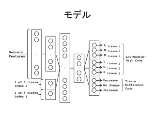
This document summarizes an experiment using deep neural networks (DNNs) to predict alternative splicing patterns in mouse tissues from RNA-seq data. The DNN model contains three hidden layers and jointly represents genomic sequence features and tissue types to predict splicing percentages and changes across tissues. Hyperparameters were optimized using 5-fold cross-validation on AUC. The trained DNN was able to accurately predict splicing patterns for 11,019 exons in 5 mouse tissues, outperforming previous models like Bayesian neural networks and multinomial logistic regression.

1. ISMB2014読み会
2014年9月11日
於：産総研CBRC

2. What
is
ISMB?
• FAQから引用
– Intelligent
Systems
for
Molecular
Biology
(ISMB)
is
the
annual
meeDng
of
the
InternaDonal
Society
for
ComputaDonal
Biology
(ISCB).
Over
the
past
eighteen
years
the
ISMB
conference
has
grown
to
become
the
largest
bioinformaDcs
conference
in
the
world.
The
ISMB
conferences
provide
a
mulDdisciplinary
forum
for
disseminaDng
the
latest
developments
in
bioinformaDcs.
ISMB
brings
together
scienDsts
from
computer
science,
molecular
biology,
mathemaDcs,
and
staDsDcs.
Its
principal
focus
is
on
the
development
and
applicaDon
of
advanced
computaDonal
methods
for
biological
problems.

3. ISMB
2014
• 開催地：米国ボストン
• 日程：7月11日-­‐15日
• プロシーディング：BioinformaDcs誌の特別号
• 採択率：
37/191
≒
19.4%
– accept
at
1st
round：
29
papers
– invite
to
2nd
round:
16
papers
– accept
at
2nd
round:
9
papers
– withdraw
aVer
acceptance:
1
paper

4. 来年は？
• ECCBと共催
⇒
ISMB/ECCB
2015
• 開催地：ダブリン＠アイルランド
• 日程：
7月10日-­‐14日
• 投稿締切：
1月9日（正月休めない！）
• 再来年以降は？
– 2016
オーランド＠米国
– 2017
プラハ＠チェコ
– 2018
シカゴ＠米国

5. ISMB2014読み会＠産総研CBRC
Vol. 30 ISMB 2014, pages i121–i129 BIOINFORMATICS doi:10.1093/bioinformatics/btu277
Deep learning of the tissue-regulated splicing code
Michael K. K. Leung1,2, Hui Yuan Xiong1,2, Leo J. Lee1,2 and Brendan J. Frey1,2,3,*
1Department of Electrical and Computer Engineering, University of Toronto, Toronto, Ontario M5S 3G4, 2Banting and
Best Department of Medical Research, University of Toronto, Toronto, Ontario M5S 3E1, Canada and 3Canadian
Institute for Advanced Research, Toronto, Ontario M5G 1Z8, Canada
ABSTRACT
Motivation: Alternative splicing (AS) is a regulated process that directs
the generation of different transcripts from single genes. A computa-tional
Previously, a ‘splicing code’ that uses a Bayesian neural net-work
慶應義塾大学理工学部
(BNN) was developed to infer a model that can predict the
outcome of AS from sequence information in different cellular
contexts (Xiong et al., 2011). One advantage of Bayesian meth-ods
佐藤健吾
model that can accurately predict splicing patterns based on
genomic features and cellular context is highly desirable, both in
understanding this widespread phenomenon, and in exploring the
effects of genetic variations on AS.
Methods: Using a deep neural network, we developed a model
inferred from mouse RNA-Seq data that can predict splicing patterns
in individual tissues and differences in splicing patterns across tissues.
Our architecture uses hidden variables that jointly represent features in
genomic sequences and tissue types when making predictions.
A graphics processing unit was used to greatly reduce the training
time of our models with millions of parameters.
is that they protect against overfitting by integrating over
models. When the training data are sparse, as is the case for
many datasets in the life sciences, the Bayesian approach can
be beneficial. It was shown that the BNN outperforms several
common machine learning algorithms, such as multinomial lo-gistic
satoken@bio.keio.ac.jp
regression (MLR) and support vector machines, for AS
prediction in mouse trained using microarray data.
There are several practical considerations when using BNNs.
They often rely on methods like Markov Chain Monte Carlo
(MCMC) to sample models from a posterior distribution,

6. AlternaDve
splicing
• ヒトにおいては、少なくとも95%の遺伝子に選
択的スプライシングが起こっている。
(wikipedia)

7. Deep
Neural
Networks
(DNN)
• 深いニューラルネットワークによる表現力
• 学習が極めて困難
Deep Neural Networks
construct
nonlinearity for hidden layers
the output layer
backpropagation does not
randomly initialized)
trained with
backpropagation (without
pretraining) perform
shallow networks

8. Deep
Neural
Networks
(DNN)
• いくつかのブレークスルー
– Autoencoderによるpre-­‐training
[Hinton
et
al.,
2006]
– Dropoutによる学習の安定化 [Srivastava
et
al.,
2014]
• 様々な分野のコンテストで圧倒的な成績
– 画像認識、音声認識、化合物の活性予測、…
• バイオインフォマティクス分野での応用はまだ
それほど多くない
– タンパク質コンタクトマップ予測 [Eickholt
et
al.,
2012]

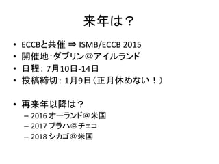
9. DNNのプレトレーニング
Stacked
Autoencoder
‡ 層ごとにオートエンコーダを学習→ 過学習を克服
± “greedy layerwise pretraining” [Hinton06]
スパースオートエンコーダ
‡ 入力サンプルをよく再現するように
± BPでor ボルツマンマシンとして学習
± 中間層がスパースに活性化するように正則化を行う
[岡谷,
2013]
• 層ごとに教師なし学習
• 各層は入力をよく再現するように学習

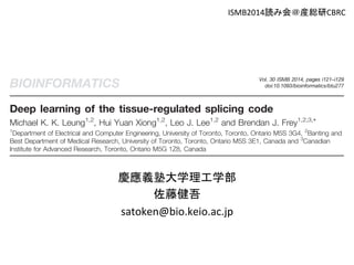
10. Dropout
• ランダムに隠れユニットを取り除いて学習
Srivastava, Hinton, Krizhevsky, Sutskever and Salakhutdinov
• アンサンブル学習と同じ効果
(a) Standard Neural Net (b) After applying dropout.
Figure 1: Dropout Neural Net Model. Left: A standard neural net with 2 hidden layers. Right:
[Srivastava
et
al.,
2014]
An example of a thinned net produced by applying dropout to the network on the left.
Crossed units have been dropped.

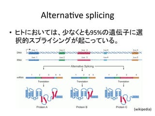
11. Deep
Neural
Networks
(DNN)
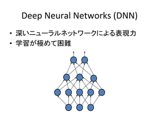
• 深いニューラルネットワークによる表現力
Neural Networks
hidden layers
not
initialized)
perform
Different Levels of Abstraction
• Hierarchical Learning
– Natural progression from low
level to high level structure as
seen in natural complexity
– Easier to monitor what is being
learnt and to guide the machine
to better subspaces
– A good lower level
representation can be used for
many distinct tasks
[Lee,
2010]

12. 問題設定
ARTICLES • エクソンがスプライシングを受けるかどうかを
予測する
features, active Information We use theory31 about the code. better than improved To assemble the compendium, parameters 300 nt 300 nt 300 nt 300 nt
RNA feature
extraction
Splicing code
5). The but diminished (Fig. 1b, code contained,a
Tissue type
Alternatively spliced exon
Feature set
Predicted change in
exon inclusion Code assembly
b
[Barash
et
al.,
2010]

13. モデル
Deep learning of of the DNN used to predict AS patterns. It contains three hidden layers, with hidden variables that jointly context (tissue types)

14. 特徴量
• 前後のエクソン・イントロンに関する1392個の特
徴量[Barash
et
al.,
2010]
300 nt 300 nt 300 nt 300 nt
ARTICLES – k-­‐mer
– 翻訳可能性
– 長さ
– 保存度
– モチーフ配列（転写因子結合部位）
– …
features, thresholds active feature Information We use a measure theory31 (see Methods). about genome-the code. A code better than guessing, improved prediction To assemble a the compendium, parameters to maximize 5). The code but diminished gains (Fig. 1b, c, based code Splicing code
contained,compendium plus did not exceed 1 a
Tissue type
Alternatively spliced exon
Feature set
Predicted change in
exon inclusion bits)
400
Final
assembled
(code
d
b
RNA feature
extraction
Code assembly

15. 出力
• PSI
(Percentage
of
Splicing
In)
[Katz
et
al.,
2010]を離
散化
– LMH
code
• Low:
0-­‐0.33,
Medium:
0.33-­‐0.66,
High:
0.66-­‐1
– DNI
code
• Decrease:
部位i
>
部位j
• No
change:
部位i
≒
部位j
（PSIの差の絶対値<0.15）
• Increase:
部位i
<
部位j
• 複数の出力を同時に学習
– 学習が安定化
1. Deep learning Architecture of the DNN used to predict AS patterns. It contains three hidden layers, with hidden variables that jointly

16. DNNの学習
• 重みは正規分布でランダムに初期化
• Stacked
Autoencoder
+
Dropout
• 細かい工夫
– 通常の確率的勾配法ではなく、部位間で差が大
きいエクソンから学習していく

17. perform well on both tasks. The optimal set of hyperparameters were then used model using both training and validation data. Five models were trained this different folds of data. Predictions made for the corresponding test data from all then evaluated and reported.
The hyperparameters that were optimized and their search ranges are: (1) the learning each of the two tasks (0.1 to 2.0), (2) the number of hidden units in each layer (30 the L1 penalty (0.0 to 0.25), (4) the standard deviation of the normal distribution initialize the weights (0.001 to 0.200), (5) the momentum schedule defined as epochs to linearly increase the momentum from 0.50 to 0.99 (50 to 1500), and (6) size (500 to 8500). The number of training epoch was fixed to 1500. In our experience, set of hyperparameters were generally found in approximately 2 days, where experiments ran on a single GPU (Nvidia GTX Titan). The selected set of hyperparameters Table S2. There is a large range of acceptable values for the number hidden units layer.
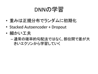
ハイパーパラメータの最適化
• 5-­‐fold
cross
validaDon：
AUCに基づき最適化
– training:
3
folds
（DNNの学習）
– validaDon:
1
fold
（ハイパーパラメータの最適化）
– test:
1
fold
（評価）
Table S2. The hyperparameters selected to train the deep neural network. Some ranges to reflect the variations from the different folds as well as hyperparameters performing runs within a given fold.
• ガウス過程に基づく
spearmint
[Snoek
et
al.,
2012]
という手法を適用
Range Selected
Hidden Units (layer 1) 450 - 650
Hidden Units (layer 2) 4500 - 6000
Hidden Units (layer 3) 400 - 600
L1 Regularization 0 - 0.05
Learning Rate (LMH code) 1.40 - 1.50
Learning Rate (DNI code) 1.80 - 2.00
Momentum Rate 1250
Minibatch Size 1500
Weight Initialization 0.05 - 0.09

18. Toronto, ON, Canada M5S 3G4
実験
• 実験環境
– Python
with
Gnumpy
[Tieleman,
2010]
で実装
– Nvidia
GTX
Titan上で実験
• データ
– マウスの５部位RNA-­‐seqデータ [Brawand
et
al.,
2011]
か
ら得た
11,019個のエクソンのスプライシングパ
ターン
1
S1 Dataset Description
The dataset consists of 11,019 mouse alternative exons in five tissue types profiled from RNA-Seq
data prepared by (Brawand et al., 2011). As explained in the main text, a distribution of
percent-spliced-in (PSI) was estimated for each exon and tissue. From this distribution, three
real-values were calculated by summing the probability mass over equally split intervals of 0 to
0.33 (low), 0.33 to 0.66 (medium), and 0.66 to 1 (high). They represent the probability that the
given exon within a tissue type has PSI value ranging from these intervals, hence are soft
assignments into each category. The models were trained using these soft labels. Table S1
shows the distribution of exons in each category, counted by selecting the label with the largest
value.
Table S1. The number of exons classified as low, medium, and high for each mouse tissue.
Exons with large tissue variability (TV) are displayed in a separate column. The proportion of
medium category exons that have large tissue variability is higher than the other two categories.
Brain Heart Kidney Liver Testis
All TV All TV All TV All TV All TV
Low 1782 579 1191 460 1287 528 1001 413 1216 452
Medium 669 456 384 330 345 294 254 220 346 270
High 5229 1068 4060 919 4357 941 3606 757 4161 887
Total 7680 2103 5635 1709 5989 1763 4861 1390 5723 1609

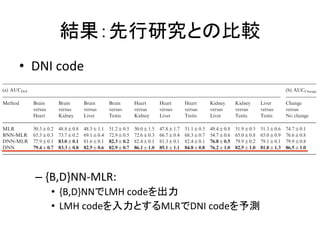
19. Heart MLR 84.6"0.1 73.1"0.3 83.6"0.1
Downloaded from http://bioinformatics.oxfordjournals.3 We present three sets of results that compare the test perform-ance
BNN 89.2"0.4 75.2"0.3 88.0"0.4
DNN 89.3"0.5 79.4"0.9 88.3"0.6
BNN 91.1"0.3 74.7"0.3 89.5"0.2
DNN 90.7"0.6 79.7"1.2 89.4"1.1
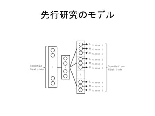
結果：先行研究との比較
RESULTS
of the BNN, DNN and MLR for splicing pattern predic-tion.
The first is the PSI prediction from the LMH code tested on
all exons. The second is the PSI prediction evaluated only on
targets where there are large Deep variations learning across of the tissues splicing for a code
given
exon. These are events where "PSI!"0.15 for at least one pair
of tissues, third result • LMH
to evaluate the tissue specificity of the model. The
shows how code
well the code (all)
can classify "PSI between
the five tissue types. Hyperparameter tuning was used in all
methods. The averaged predictions from all partitions and
folds are used to evaluate the model’s performance on their cor-responding
Kidney MLR 86.7"0.1 75.6"0.2 86.3"0.1
BNN 92.5"0.4 78.3"0.4 91.6"0.4
DNN 91.9"0.6 82.6"1.1 91.2"0.9
Liver MLR 86.5"0.2 75.6"0.2 86.5"0.1
BNN 92.7"0.3 77.9"0.6 92.3"0.5
DNN 92.2"0.5 80.5"1.0 91.1"0.8
• LMH
code
(high
Dssue
Testis MLR 85.6"0.1 72.3"0.4 85.2"0.1
BNN 91.1"0.3 75.5"0.6 90.4"0.3
DNN 90.7"0.6 76.6"0.7 89.7"0.7
variability)
Table 1. Comparison of the LMH code’s AUC performance on different
methods
(a) AUCLMH_All
test dataset. Similar to training, we tested on exons
and tissues that have at least 10 junction reads.
For the LMH code, as the same prediction target can be gen-erated
Tissue Method Low Medium High
by different input configurations, and there are two LMH
Brain MLR 81.3"0.1 72.4"0.3 81.5"0.1
outputs, we BNN compute the 89.2predictions "0.4 for 75.2all "input 0.3 combinations
88.0"0.4
containing DNN the particular 89.3tissue "0.5 and average 79.4"them 0.9 into 88.3a single
"0.6
prediction for testing. To assess the stability of the LMH predic-tions,
Heart MLR 84.6"0.1 73.1"0.3 83.6"0.1
BNN 91.1"0.3 74.7"0.3 89.5"0.2
DNN 90.7"0.6 79.7"1.2 89.4"1.1
we calculated the percentage of instances in which there is
a prediction from one tissue input configuration that does not
agree with another tissue input configuration in terms of class
membership, for all exons and tissues. Of all predictions, 91.0%
agreed with each other, 4.2% have predictions that are in adja-cent
Kidney MLR 86.7"0.1 75.6"0.2 86.3"0.1
BNN 92.5"0.4 78.3"0.4 91.6"0.4
DNN 91.9"0.6 82.6"1.1 91.2"0.9
Liver MLR 86.5"0.2 75.6"0.2 86.5"0.1
classes (i.e. low and medium, or medium and high), and 4.8%
BNN 92.7"0.3 77.9"0.6 92.3"0.5
DNN 92.2"0.5 80.5"1.0 91.1"0.8
otherwise. Of those predictions that agreed with each other,
85.9% correspond to the correct class label on test data,
51.2% for the predictions with adjacent classes and 53.8% for
the remaining predictions. This information can be used to assess
the confidence of the predicted class labels. Note that predictions
spanning adjacent classes may be indicative that the PSI value is
somewhere between the two classes, and the above analysis using
hard class labels can underestimate the confidence of the model.
Testis MLR 85.6"0.1 72.3"0.4 85.2"0.1
BNN 91.1"0.3 75.5"0.6 90.4"0.3
DNN 90.7"0.6 76.6"0.7 89.7"0.7
(b) AUCLMH_TV
BNN：Bayeisian
NN
[Xiong
et
al.,
2011],
MLR:
MulDnomial
LogisDc
Regression
Tissue Method Low Medium High
(b) AUCLMH_TV
Tissue Method Low Medium High
Brain MLR 71.1"0.2 58.8"0.2 70.8"0.1
BNN 77.9"0.5 61.1"0.5 76.5"0.7
DNN 82.8"1.0 69.5"1.1 81.1"0.4
Heart MLR 73.9"0.3 58.6"0.4 72.7"0.1
BNN 78.1"0.3 58.9"0.3 75.7"0.3
DNN 82.0"1.1 67.4"1.3 79.7"1.2
Kidney MLR 79.7"0.3 64.3"0.2 79.4"0.2
BNN 83.9"0.5 66.4"0.5 83.3"0.6
DNN 86.2"0.6 73.2"1.3 85.3"1.2
Liver MLR 80.1"0.5 63.7"0.3 79.4"0.3
BNN 84.9"0.7 65.4"0.7 84.4"0.7
DNN 87.7"0.6 69.4"1.2 84.8"0.8
Testis MLR 77.3"0.2 60.8"0.3 77.0"0.1
BNN 81.1"0.5 63.9"0.9 81.0"0.5
DNN 84.6"1.1 67.8"0.9 83.5"0.9
Notes: " indicates 1 standard deviation; top performances are shown in bold.
subset of events that exhibit large tissue variability. Here, the
DNN significantly outperforms the BNN in all categories and

20. 先行研究のモデル
S3 Model Architectures
Genomic
Features
…
…
L tissue 1
M tissue 1
H tissue 1
L tissue 2
M tissue 2
H tissue 2
L tissue 5
M tissue 5
H tissue 5
…
Low-Medium-
High Code
Fig. S3. Architecture of the Bayesian neural network (Xiong et al., 2011) used for comparison,
where low-medium-high predictions are made separately for each tissue.
L tissue i

21. 結果：先行研究との比較
• DNI
code
Table 2. Comparison of the DNI code’s performance in terms of the AUC for decrease versus increase (AUCDvI) and change versus no change
(AUCChange)
(a) AUCDvI (b) AUCChange
– {B,D}NN-­‐MLR:
Table 2a shows the AUCDvI for classifying decrease versus
increase inclusion for all and DNN outperform • {pairs of tissue. Both the B,D}BNN-NNMLR でLMH
the DNN-MLR
by a good margin.
Comparing the DNN with DNN-MLR, the DNN shows some
gain in differentiating brain and heart AS patterns from other
tissues. The performance of differentiating the remaining tissues
(kidney, liver and testis) with each other is similar between the
DNN and DNN-MLR. We note that the similarity between the
DNN and DNN-MLR in terms of performance can be due to
the use of soft labels for training. Using MLR directly on the
codeを出力
• LMH
codeを入力とするMLRでDNI
codeを予測
Method Brain
versus
Heart
Brain
versus
Kidney
Brain
versus
Liver
Brain
versus
Testis
Heart
versus
Kidney
Heart
versus
Liver
Heart
versus
Testis
Kidney
versus
Liver
Kidney
versus
Testis
Liver
versus
Testis
Change
versus
No change
MLR 50.3"0.2 48.8"0.8 48.3"1.1 51.2"0.5 50.0"1.5 47.8"1.7 51.1"0.5 49.4"0.8 51.9"0.5 51.3"0.6 74.7"0.1
BNN-MLR 65.3"0.3 73.7"0.2 69.1"0.4 72.9"0.5 72.6"0.3 66.7"0.4 68.3"0.7 54.7"0.6 65.0"0.8 65.0"0.9 76.6"0.8
DNN-MLR 77.9"0.1 83.0"0.1 81.6"0.1 82.3"0.2 82.4"0.1 81.3"0.1 82.4"0.1 76.8"0.5 79.9"0.2 79.1"0.1 79.9"0.8
DNN 79.4"0.7 83.3"0.8 82.5"0.6 82.9"0.7 86.1"1.0 85.1"1.1 84.8"0.8 76.2"1.0 82.5"1.0 81.8"1.3 86.5"1.0
Note: " indicates 1 standard deviation; top performances are shown in bold.
Table 3. Performance of the DNN evaluated on a different RNA-Seq
experiment
(a) AUCLMH_All
Tissue Low Medium High
Brain 88.1"0.5 76.1"1.0 87.0"0.6
Heart 90.7"0.5 78.4"1.3 89.0"1.0
M.K.K.Leung et al.

22. 結果：重要な特徴量
K.K.Leung et al.

23. まとめ
• DNNを用いてスプライシングパターンを高精
度に予測する手法を開発した。
• 適切な学習方法を用いることで、スパースな
データにおいてもDNNで学習できることを示し
た。

24. 感想
• この論文がなぜISMBに採択されたか？
– 今流行のDeep
Learningを使っている。
– 問題設定自体は昔からあるものだけれど、それ
を最新の手法を使ってうまく解いた。
– 複数の出力を同時に学習する転移学習的なモデ
ルにしているところは斬新かも。

25. 感想
• DNNはバイオインフォマティクス分野で流行るか？
– 研究され尽くされている分野では、期待するほどの改善
は見られない。（e.g.
自然言語処理の一部の分野）
– パラメータがどうしても多くなるから、データ数はそれなり
に必要になる。⇒
オミクス計測技術
– 同時に、計算量が膨大になる。⇒
GPGPU
– 生物よりの研究者が気軽に使える実装があまりない。
⇒
Python
with
Theano
– ハイパーパラメータの選択が大変
⇒
暇人しか手を出せない。
⇒
SVMほどは流行らないのでは？