Cornell Pbsb 20090126 Nets

Understanding Protein Function on a Genome-scale through the Analysis of Molecular Networks Mark B Gerstein Yale Slides at Lectures.GersteinLab.org (See Last Slide for References & More Info.) (c) Mark Gerstein, 2002, Yale, bioinfo.mbb.yale.edu

The problem: Grappling with Function on a Genome Scale? 250 of ~530 originally characterized on chr. 22 [Dunham et al. Nature (1999)] >25K Proteins in Entire Human Genome (with alt. splicing) .…… ~530

Traditional single molecule way to integrate evidence & describe function Descriptive Name: Elongation Factor 2 Summary sentence describing function: This protein promotes the GTP-dependent translocation of the nascent protein chain from the A-site to the P-site of the ribosome. EF2_YEAST Lots of references to papers

Some obvious issues in scaling single molecule definition to a genomic scale Fundamental complexities Often >2 proteins/function Multi-functionality: 2 functions/protein Role Conflation: molecular, cellular, phenotypic

Some obvious issues in scaling single molecule definition to a genomic scale Fundamental complexities Often >2 proteins/function Multi-functionality: 2 functions/protein Role Conflation: molecular, cellular, phenotypic Fun terms… but do they scale?.... Starry night (P Adler, ’94) [Seringhaus et al. GenomeBiology (2008)]

Hierarchies & DAGs of controlled-vocab terms but still have issues... [Seringhaus & Gerstein, Am. Sci. '08] GO (Ashburner et al.) MIPS (Mewes et al.)

Towards Developing Standardized Descriptions of Function Subjecting each gene to standardized expt. and cataloging effect KOs of each gene in a variety of std. conditions => phenotypes Std. binding expts for each gene (e.g. prot. chip) Function as a vector Interaction Vectors [Lan et al, IEEE 90:1848]

Networks (Old & New) [Seringhaus & Gerstein, Am. Sci. '08] Classical KEGG pathway Same Genes in High-throughput Network

Networks occupy a midway point in terms of level of understanding 1D: Complete Genetic Partslist ~2D: Bio-molecular Network Wiring Diagram 3D: Detailed structural understanding of cellular machinery [Jeong et al. Nature, 41:411] [Fleischmann et al., Science, 269 :496]

Networks as a universal language Disease Spread [Krebs] Protein Interactions [Barabasi] Social Network Food Web Neural Network [Cajal] Electronic Circuit Internet [Burch & Cheswick]

Networks as a Central Theme in Systems Biology Reductionist Approach Integrative Approach [Adapted from H Yu] Systems Biology

Interactome networks Network pathology & pharmacology [Adapted from H Yu] Breast Cancer Parkinson’s Disease Alzheimer’s Disease Multiple Sclerosis

Using the position in networks to describe function [NY Times, 2-Oct-05, 9-Dec-08]

Types of Networks Interaction networks [Horak, et al, Genes & Development, 16:3017-3033] [DeRisi, Iyer, and Brown, Science, 278:680-686] [Jeong et al, Nature, 41:411] Regulatory networks Metabolic networks Nodes: proteins or genes Edges: interactions

Combining networks forms an ideal way of integrating diverse information Metabolic pathway Transcriptional regulatory network Physical protein-protein Interaction Co-expression Relationship Part of the TCA cycle Genetic interaction (synthetic lethal) Signaling pathways

Outline Predicting Networks Training set expansion Properties of Protein Networks Hubs Dynamics of Networks Dynamics across cellular states Dynamics across environments Protein Networks and Human Variation

Predicting Networks How do we construct large molecular networks? From extrapolating correlations between functional genomics data with fairly small sets of known interactions, making best use of the known training data.

Network Prediction Figure 6: A map of known and a subset of predicted interactions among helical membrane proteins. Nodes represent helical membrane proteins, and edges represent interactions among them. Red edges represent known interactions that are also predicted to interact, blue edges represent other known interactions, and green edges represent ~700 top interaction predictions (ranked by descending logistic regression score) out of a total of 4,145. Purple nodes represent helical membrane proteins that show up in the known interactions, and green nodes represent new helical membrane proteins. New K n o w n Ex. of Predicted Membrane Protein Interactome in Xia et al. JMB (2006) Only small portions are already known Many other kinds of data available  Use them to learn models for predicting the unknown portions

Example: yeast PPI network Actual size: ~6,000 nodes  Computational cost: ~18M pairs Estimated ~15,000 edges  Sparseness: 0.08% of all pairs (Yu et al., 2008) Known interactions: Small-scale experiments: accurate but few  Overfitting: ~5,000 in BioGRID, involving ~2,300 proteins Large-scale experiments: abundant but noisy  Noise: false +ve/-ve for yeast two-hybrid data up to 45% and 90% (Huang et al., 2007)

Learning Concepts in machine learning: Training sets: Positive set: known interactions Negative set: known non-interactions Features: Data describing the objects Model: A function that takes two objects as input and predicts whether they interact

Training sets Known interactions Known non-interactions Unknown 1 2 4 3 1 2 3 4 1 0 1 ? 1 2 1 ? 0 ? 3 ? 0 ? ? 4 1 ? ? ?

Features Example 1: gene expression x 1 = (0.2, 2.4, 1.5, …) x 2 = (0.8, 2.2, 1.5, …) x 3 = (4.3, 0.1, 7.5, …) … sim(x 1 , x 2 ) = 0.62 sim(x 1 , x 3 ) = -0.58 … Gasch et al., 2000 1 2 4 3 Similarity scale: 1 -1

Features Example 2: sub-cellular localization x 1 = (1, 1, 0, 0, …) x 2 = (1, 1, 1, 0, …) x 3 = (1, 0, 1, 0, …) … sim(x 1 , x 2 ) = 0.81 sim(x 1 , x 3 ) = 0.12 … Similarity scale: 1 -1 http://www.scq.ubc.ca/wp-content/yeasttwohybridtranscript.gif 1 2 4 3

Data integration & Similarity Matrix 1 2 4 3 1 2 4 3 1 2 4 3 1 2 4 3 1 2 3 4 1 1.00 0.57 0.55 0.40 2 0.57 1.00 0.66 0.89 3 0.55 0.66 1.00 0.79 4 0.40 0.89 0.79 1.00

Evaluation Computational: Cross-validation Indirect evidence (e.g. same GO category) Experimental: Validation of de novo predictions

Learning methods An endless list: Docking (e.g. Schoichet and Kuntz 1991) Evolutionary (e.g. Ramani and Marcotte, 2003) Topological (e.g. Yu et al., 2006) Bayesian (e.g. Jansen et al., 2003) Kernel methods Global modeling: em (Tsuda et al., 2003) kCCA (Yamanishi et al., 2004) kML (Vert and Yamanishi, 2005) Pairwise kernel (Pkernel) (Ben-Hur and Noble, 2005) Local modeling: Local modeling (Bleakley et al., 2007) … Let’s compare fairly in a public challenge! (DREAM)

Kernels Kernel: a similarity matrix that is positive semi-definite (p.s.d.) Objects in an feature space 2 1 3 4 Good for integrating heterogeneous datasets (protein sequences, PSSM, gene expression, …) – no need to explicitly place them in a common feature space Similarity matrix Compute inner products p.s.d. implies

Kernel methods Use the kernel as proxy to work in the feature space Example: SVM (finding the best separating hyperplane) The only thing that we need to know about the objects: their similarity values (inner products) Maximize Subject to Equivalent to 2 1 3 4

Kernel methods for predicting networks: local vs. global modeling Local modeling: build one model for each node Model for node 3: Problem: insufficient and unevenly distributed training data (what if node 3 has no known interactions at all?) 1 2 4 3 ? 1 2 4 3 2 4

Kernel methods for predicting networks: local vs. global modeling Global modeling: build one model for the whole network Pairwise kernel: consider object pairs instead of individual objects Problem: O(n 2 ) instances, O(n 4 ) kernel elements Direct methods: threshold the kernel to make predictions Problem: One single global model, may not be able to handle subclasses 1 2 4 3 ? 1 3 2 3 2 4 1 4 1 2 3 4 1 1 4 4 2 2 3 3 1 4 1 2 3 4 4 4 2 2 3 3 1 2 3 4 1 1.00 0.57 0.55 0.40 2 0.57 1.00 0.66 0.89 3 0.55 0.66 1.00 0.79 4 0.40 0.89 0.79 1.00 Threshold: 0.7 1 2 3 4 1 1.00 0.57 0.55 0.40 2 0.57 1.00 0.66 0.89 3 0.55 0.66 1.00 0.79 4 0.40 0.89 0.79 1.00

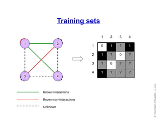
Our work: training set expansion Goal: Utilize the flexibility of local modeling Tackle the problem of insufficient training data Idea: generate auxiliary training data Prediction propagation Kernel initialization [Yip and Gerstein, Bioinformatics ('09, in press)]

Prediction propagation Motivation: some objects have more examples than others Our approach: Learn models for objects with more examples first Propagate the most confident predictions as auxiliary examples of other objects [Yip and Gerstein, Bioinformatics ('09, in press)] 1 2 4 3 1 2 4 3 1 2 4 3 1 2 4 3 1 2 4 3

Kernel initialization Motivation: what if most objects have very few examples? Our approach (inspired by the direct method): Add the most similar pairs in the kernel as positive examples Add the most dissimilar pairs in the kernel as negative examples [Yip and Gerstein, Bioinformatics ('09, in press)] 1 2 4 3 1 2 3 4 1 1.00 0.57 0.55 0.40 2 0.57 1.00 0.66 0.89 3 0.55 0.66 1.00 0.79 4 0.40 0.89 0.79 1.00 1 2 4 3

Remarks Can be used in combination Prediction propagation theoretically related to co-training (Blum and Mitchell, 1998) Semi-supervised Similarity with PSI-BLAST Algorithm complexity O(nf(n)) of local modeling vs. O(f(n 2 )) of global modeling [Yip and Gerstein, Bioinformatics ('09, in press)]

Experiments Gold-standard interactions: BioGRID, from studies that report less than 10 interactions Features: [Yip and Gerstein, Bioinformatics ('09, in press)] Code Data type Source Kernel phy Phylogenetic profiles COG v7 (Tatusov et al., 1997) RBF (  =3,8) loc Sub-cellular localization (Huh et al., 2003) Linear exp-gasch Gene expression (environmental response) (Gasch et al., 2000) RBF (  =3,8) exp-spellman Gene expression (cell-cycle) (Spellman et al., 1998) RBF (  =3,8) y2h-ito Yeast two-hybrid (Ito et al., 2000) Diffusion (  =0.01) y2h-uetz Yeast two-hybrid (Uetz et al., 2000) Diffusion (  =0.01) tap-gavin Tandem affinity purification (Gavin et al., 2006) Diffusion (  =0.01) tap-krogan Tandem affinity purification (Krogan et al., 2006) Diffusion (  =0.01) int Integration Summation

Prediction accuracy Observations: Highest accuracy by training set expansion Overfitting of local modeling without training set expansion Comparing prediction propagation and kernel initialization [Yip and Gerstein, Bioinformatics ('09, in press)]

Complementarity of the two methods [Yip and Gerstein, Bioinformatics ('09, in press)]

Network Dynamics #1: Cellular States How do networks change across different cellular states? How can this be used to assign function to a protein?

Global topological measures Indicate the gross topological structure of the network Degree ( K ) Path length ( L ) Clustering coefficient ( C ) [Barabasi] Interaction and expression networks are undirected 5 2 1/6

Global topological measures for directed networks In-degree Regulatory and metabolic networks are directed Out-degree 5 3 TFs Targets

Scale-free networks Hubs dictate the structure of the network log(Degree) log(Frequency) Power-law distribution [Barabasi]

Hubs tend to be Essential Essential Non- Essential Integrate gene essentiality data with protein interaction network. Perhaps hubs represent vulnerable points? [ Lauffenburger, Barabasi] "hubbiness" [Yu et al., 2003, TIG]

Relationships extends to "Marginal Essentiality" Essential Not important Marginal essentiality measures relative importance of each gene (e.g. in growth-rate and condition-specific essentiality experiments) and scales continuously with "hubbiness" important Very important "hubbiness" [Yu et al., 2003, TIG]

Analyzed network as a static entity But network is dynamic Different sections of the network are active under different cellular conditions Integrate gene expression data Target Genes Transcription Factors Dynamic Yeast TF network Luscombe et al. Nature 431: 308

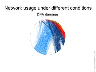
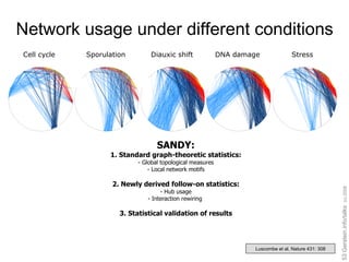
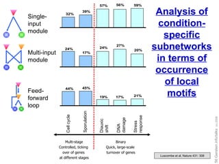
Gene expression data for five cellular conditions in yeast Multi-stage Binary [Brown, Botstein, Davis….] Cellular condition Cell cycle Sporulation Diauxic shift DNA damage Stress response

Backtracking to find active sub-network Active regulatory sub-network Define differentially expressed genes Identify TFs that regulate these genes Identify further TFs that regulate these TFs

Network usage under different conditions static Luscombe et al. Nature 431: 308

Network usage under different conditions cell cycle

Network usage under different conditions sporulation

Network usage under different conditions diauxic shift

Network usage under different conditions DNA damage

Network usage under different conditions stress response

SANDY: 1. Standard graph-theoretic statistics: - Global topological measures - Local network motifs 2. Newly derived follow-on statistics: - Hub usage - Interaction rewiring 3. Statistical validation of results Network usage under different conditions Cell cycle Sporulation Diauxic shift DNA damage Stress Luscombe et al. Nature 431: 308

SANDY: 1. Standard graph-theoretic statistics: - Global topological measures - Local network motifs 2. Newly derived follow-on statistics: - Hub usage - Interaction rewiring 3. Statistical validation of results Network usage under different conditions Cell cycle Sporulation Diauxic shift DNA damage Stress

Analysis of condition-specific subnetworks in terms of global topological statistics Luscombe et al. Nature 431: 308 Sporulation Cell cycle Diauxic shift DNA damage Stress response Outdegree Indegree Pathlength Clustering coefficient Binary Quick, large-scale turnover of genes Multi-stage Controlled, ticking over of genes at different stages

Analysis of condition-specific subnetworks in terms of occurrence of local motifs Luscombe et al. Nature 431: 308 Sporulation Cell cycle Diauxic shift DNA damage Stress response Single-input module Multi-input module Feed-forward loop Binary Quick, large-scale turnover of genes Multi-stage Controlled, ticking over of genes at different stages

Summary multi-stage conditions binary conditions Cell cycle Sporulation Diauxic shift DNA damage Stress less pronounced Hubs more pronounced longer Path Lengths shorter more TF inter-regulation less complex loops (FFLs) Motifs simpler (SIMs)

Transient Hubs Regulatory hubs Luscombe et al. Nature 431: 308 Questions: Do hubs stay the same or do they change over between conditions? Do different TFs become important? Our Expectations Literature: Hubs are permanent features of the network regardless of condition Random networks (sampled from complete regulatory network) Random networks converge on same TFs 76-97% overlap in TFs classified as hubs ( ie hubs are permanent)

Some permanent hubs house-keeping functions Most are transient hubs Different TFs become key regulators in the network Implications for condition-dependent vulnerability of network Luscombe et al. Nature 431: 308 transitient hubs permanent hubs transient hubs permanent hubs cell cycle sporulation diauxic shift DNA damage stress response all conditions

Luscombe et al. Nature 431: 308 transitient hubs permanent hubs Swi4, Mbp1 Ime1, Ume6 Msn2, Msn4 cell cycle sporulation diauxic shift DNA damage stress response all conditions

Luscombe et al. Nature 431: 308 transitient hubs permanent hubs Unknown functions cell cycle sporulation diauxic shift DNA damage stress response all conditions

Network Dynamics #2: Environments How do molecular networks change across environments? What pathways are used more ? Used as a biosensor ?

Comparative Metagenomics Water Soil Do the proportions of pathways represented in these two samples differ? Dinsdale et. al., Nature 2008

Trait-based Biogeography Green et. al., Science 2008 Average Yearly Rainfall (mm) Leaf span Leaf area Do the proportions of pathways represented in these two samples CHANGE as a function of their environments? Long Island Sound, CT Charles River, MA

Global Ocean Survey Statistics (GOS) 6.25 GB of data 7.7M Reads 1 million CPU hours to process Rusch, et al., PLOS Biology 2007

Expressing data as matrices indexed by site, env. var., and pathway usage Pathway Sequences (Community Function) Environmental Features [Rusch et. al., (2007) PLOS Biology; Gianoulis et al., PNAS (in press, 2009]

Simple Relationships: Pairwise Correlations [ Gianoulis et al., PNAS (in press, 2009) ] Pathways

Canonical Correlation Analysis: Simultaneous weighting [ Gianoulis et al., PNAS (in press, 2009) ] + b’ + c’ GPI = a’ + b + c UPI = a

Canonical Correlation Analysis: Simultaneous weighting [ Gianoulis et al., PNAS (in press, 2009) ] + b’ + c’ GPI = a’ + b + c UPI = a Metabolic Pathways Environmental Features Temp Chlorophyll etc Photosynthesis Lipid Metabolism etc

Environmental-Metabolic Space The goal of this technique is to interpret cross-variance matrices We do this by defining a change of basis. [ Gianoulis et al., PNAS (in press, 2009) ] a,b

Circuit Map Environmentally invariant Environmentally variant Strength of Pathway co-variation with environment [ Gianoulis et al., PNAS (in press, 2009) ]

Conclusion #1: energy conversion strategy, temp and depth [ Gianoulis et al., PNAS (in press, 2009) ]

Conclusion #2: Outer Membrane components vary the environment [ Gianoulis et al., PNAS (in press, 2009) ]

Conclusion #3: Covariation of AA biosynthesis and Import Why is their fluctuation in amino acid metabolism? Is there a feature(s) that underlies those that are environmentally-variant as opposed to those which are not? [ Gianoulis et al., PNAS (in press, 2009) ]

Conclusion #4: Cofactor (Metal) Optimization Methionine degradation Polyamine biosynthesis Spermidine/Putrescine transporters Methionine synthesis Cobalamin biosynthesis Cobalt transporters Methionine Salvage IS DEPENDENT-ON Methionine IS NEEDED FOR S-adenosyl Methionine Biosynthesis (synthesize SAM one of the most important methyl donors) RELIES ON Arg/His/Ornithine transporters Methionine salvage, synthesis, and uptake, transport [ Gianoulis et al., PNAS (in press, 2009) ]

Biosensors: Beyond Canaries in a Coal Mine [ Gianoulis et al., PNAS (in press, 2009) ]

Networks & Variation Which parts of the network vary most in sequence? Which are under selection, either positive or negative?

METHODOLOGY: MAP SNP AND CNV DATA ONTO ENSEMBL GENES, AND THEN MAP ENSEMBL GENES TO THE KNOWN INTERACTOME * From Nielsen et al. PLoS Biol. (2005) and Bustamante et al. Nature (2005) Source: PMK ILLUSTRATIVE Hapmap/Perlegen ENSG000XXXX: rsSNP00XXX CNV_XXX DN/DS XXXX Recombination rate Map to ENSEMBL genes Interactome SNPs ~30000 interactions from HPRD and Y2H screens Database of Genomic Variants Map to proteins in the interaction network Ensembl Genes Dataset of network position / parameters (e.g. degree centrality or betweenness centrality) in relationship to SNPs, CNV’s, recombination rates and positive selection tests Result CNVs + SDs

ADAPTIVE EVOLUTION CAN BE SEEN ON TWO DIFFERENT LEVELS Intra-species variation Fixed mutations (differences to other species) Single- basepair Structural variation Copy Number Variants Single-Nucleotide Polymorphisms Segmental Duplications Fixed Differences Source: PMK Positive Selection Positive Selection

POSITIVE SELECTION LARGELY TAKES PLACE AT THE NETWORK PERIPHERY Source: Nielsen et al. PLoS Biol. (2005), HPRD, and Kim et al. PNAS (2007) High likelihood of positive selection Lower likelihood of positive selection Not under positive selection No data about positive selection Positive selection in the human interactome

CENTRAL PROTEINS ARE LESS LIKELY TO BE UNDER POSITIVE SELECTION Peripheral genes are likely to under positive selection, whereas hubs aren’t This is likely due to the following reasons: Hubs have stronger structural constraints, the network periphery doesn’t Most recently evolved functions (e.g. “environmental interaction genes” such as sensory perception genes etc.) would probably lie in the network periphery Effect is independent of any bias due to gene expression differences Degree vs. Positive Selection Reasoning * With a probability of over 80% to be positively selected as determined by Ka/Ks. Other tests of positive selection (McDonald Kreitmann and LDD) corroborate this result. Source: Nielsen et al. PLoS Biol. (2005), Bustamante et al. Nature (2005), HPRD, Rual et al. Nature (2005), and Kim et al. PNAS (2007) Hubs

CENTRAL NODES ARE LESS LIKELY TO LIE INSIDE OF SDs This result also confirms our initial hypothesis – peripheral nodes tend to lie in regions rich in SDs. Since segmental duplications are a different mechanism of ongoing evolution, the less constrained peripheral proteins are enriched in them. Note that despite the small size of our dataset for known SD’s we get significant correlations. It is to be expected that the correlations will get clearer as more data emerges* Centrality vs. SD occurrence Reasoning * Specifically, a number of the SDs are likely not fixed, but rather common CNVs in the reference genome Source: Database of genetic variation, HPRD, Rual et al. Nature (2005), and Kim et al. PNAS (2007)

BURIED SITES ARE CONSERVED AND MUCH LESS LIKELY TO HARBOR NON-SYNONYMOUS MUTATIONS p<<0.01 Buried sites dN/dS Ratio Exposed sites p<<0.01 Site with Synonymous Mutations only Sites with Non-synonymous Mutations Average Relative Surface Exposure Source: Kim et al. PNAS (2007) Why do we observer this? Perhaps central hub proteins are involved in more interactions & have more surface buried.

Another explanation: THE NETWORK PERIPHERY CORRESPONDS TO THE CELLULAR PERIPHERY Chromosome Nucleus Cytoplasm Membrane Extracellular Region Betweenness Centrality (x 10 4 ) Degree Centrality Source: Gandhi et al. ( Nature Genetics 2006), Kim et al. PNAS (2007)

IS RELAXED CONSTRAINT OR ADAPTIVE EVOLUTION THE REASON FOR THE PREVALENCE OF BOTH SELECTED GENES AND SDs AT THE NETWORK PERIPHERY? Source: Kim et al. PNAS (2007) Relaxed Constraint Adaptive Evolution ILLUSTRATIVE Increases inter-species variation – more variable loci are under less negative selection Can be seen in higher Ka/Ks ratio or SD occurrence Inter-Species Variation (Fixed differences) Intra-Species Variation (Polymorphisms) Increases intra-species variation – for the very same reason Can be seen in both SNPs or CNVs Increases inter-species variation – more variable loci are under less negative selection Can be seen in higher Ka/Ks ratio or SD occurrence Should not have effects on intra-species variation

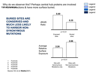
SOME, BUT NOT ALL OF THE SINGLE-BASEPAIR SELECTION AT THE PERIPHERY IS DUE TO RELAXED CONSTRAINT There is a difference in variability (in terms of SNPs) between the network periphery and the center However, this difference is much smaller than the difference in selection This most likely means, that part of the effect we’re seeing is due to relaxed constraint (and higher variability) But, not the entire effect* Inter vs. Intra-Species Variation in Networks Reasoning * But it’s hard to quantify Source: Kim et al. (2007) PNAS Inter-Species (Fixed differences) Intra-Species (SNPs) [ Variability ]

Similar Results for Large-scale Genomic Changes (CNVs and SDs) There a small difference in variability (in terms of CNVs) between the network periphery and the center But, there is a (as shown before) marked difference in fixed (and hence, presumably, selected) SDs at the network periphery and center Inter vs. Intra-Species Variation in Networks Reasoning Source: Kim et al. (2007) PNAS Inter-Species (SDs) Intra-Species (CNVs) [ Variability ]

Conclusions: Net Intro. + Predicting Networks Developing Standardized Descriptions of Protein Function Gene Naming Predicting Networks Extrapolating from the Training Set Principled ways of using the training set data in the fullest possible fashion Prediction Propagation Kernel Initialization

Conclusions: Network Dynamics across Cellular States Merge expression data with Networks Active network markedly different in different conditions Identify transient hubs associated with particular conditions Use these to annotate genes of unknown function

Conclusions: Networks Dynamics across Environments Developed and adapted techniques to connect quantitative features of environment to metabolism. Applied to available aquatic datasets, we identified footprints that were predictive of their environment (potentially could be used as biosensor). Strong correlation exists between a community’s energy conversion strategies and its environmental parameters (e.g. temperature and chlorophyll). Suggest that limiting amounts of cofactor can (partially) explain increased import of amino acids in nutrient-limited conditions.

Conclusions: Connecting Networks & Human Variation We find ongoing evolution (positive selection) at the network periphery. This trend is present on two levels: On a sequence level, it can be seen as positive selection of peripheral nodes On a structural level, it can be seen as the pattern of SDs that display significantly higher allele frequencies in non-central genes 2 possible mechanisms for this : adaptive evolution at cellular periphery & relaxation of structural constraints at the network periphery We show that the latter can only explain part of the increased variability,,,

TopNet – an automated web tool [Yu et al., NAR (2004); Yip et al. Bioinfo. (2006); Similar tools include Cytoscape.org, Idekar, Sander et al] (vers. 2 : " TopNet -like Yale Network Analyzer") Normal website + Downloaded code (JAVA) + Web service (SOAP) with Cytoscape plugin

(c) Mark Gerstein, 2002, Yale, bioinfo.mbb.yale.edu TopNet.GersteinLab.org Acknowledgements MG MS

Acknowledgements TopNet.GersteinLab.org (c) Mark Gerstein, 2002, Yale, bioinfo.mbb.yale.edu MS MG

Acknowledgements TopNet.GersteinLab.org (c) Mark Gerstein, 2002, Yale, bioinfo.mbb.yale.edu H Yu P Kim K Yip J Lu S Douglas M Seringhaus Y Xia T Gianoulis J Korbel A Sboner P Patel P Cayting P Bork, J Raes Job opportunities currently for postdocs & students N Luscombe A Paccanaro S Teichmann M Babu MS MG

DPM: Discriminative Partition Matching Cluster (Partition) Test Environment Metabolism Taurine biosynthesis Heme biosynthesis Asparagine degradation Nitrogen fixation Acylglycerol degradation Asparagine biosynthesis Cysteine Metabolism pval Functional class [ Gianoulis et al., PNAS (in press, 2009) ] InfoStorage & Processing .07 Cellular Process .08 Metabolism 4x10-14

Interactome [From H Yu] protein-DNA interactions protein-protein interactions PROTEOME GENOME Citrate Cycle METABOLISM Protein-small molecule interactions

Networks help us understand biological processes [From H Yu]

More Information on this Talk TITLE : Understanding Protein Function on a Genome-scale through the Analysis of Molecular Networks SUBJECT: Networks DESCRIPTION : Cornell Medical School, Physiology, Biophysics and Systems Biology (PBSB) graduate program, 2009.01.26, 16:00-17:00; [I: CORNELL-PBSB ] (Long networks talk, incl. the following topics: why networks w. amsci*, funnygene*, net. prediction intro, memint*, tse*, essen*, sandy*, metagenomics*, netpossel*, tyna*+ topnet*, & pubnet* . Fits easily into 60’ w. 10’ questions. PPT works on mac & PC and has many photos w. EXIF tag kwcornellpbsb .) (Paper references in the talk were mostly from Papers.GersteinLab.org. The above topic list can be easily cross-referenced against this website. Each topic abbrev. which is starred is actually a papers “ID” on the site. For instance, the topic pubnet * can be looked up at http://papers.gersteinlab.org/papers/ pubnet ) PERMISSIONS : This Presentation is copyright Mark Gerstein, Yale University, 2008. Please read permissions statement at http://www.gersteinlab.org/misc/permissions.html . Feel free to use images in the talk with PROPER acknowledgement (via citation to relevant papers or link to gersteinlab.org). . PHOTOS & IMAGES . For thoughts on the source and permissions of many of the photos and clipped images in this presentation see http://streams.gerstein.info . In particular, many of the images have particular EXIF tags, such as kwpotppt , that can be easily queried from flickr, viz: http://www.flickr.com/photos/mbgmbg/tags/ kwpotppt .

Cornell Pbsb 20090126 Nets

More Related Content

What's hot

Viewers also liked

Similar to Cornell Pbsb 20090126 Nets

Recently uploaded

Cornell Pbsb 20090126 Nets