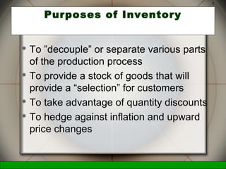
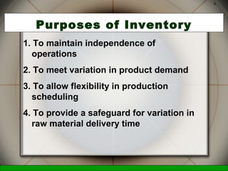
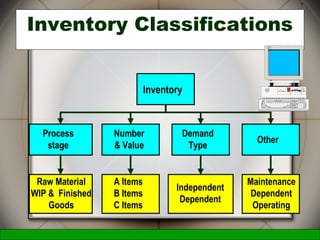
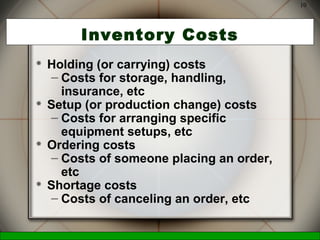
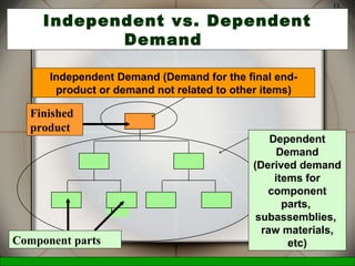
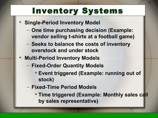
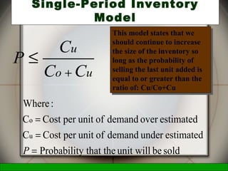
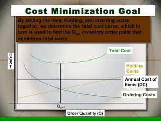
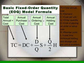
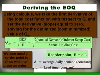
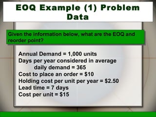
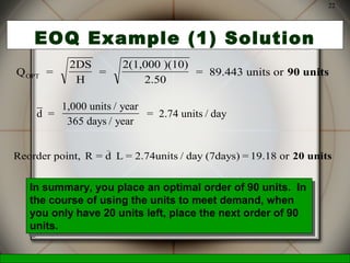
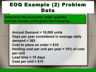
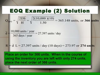
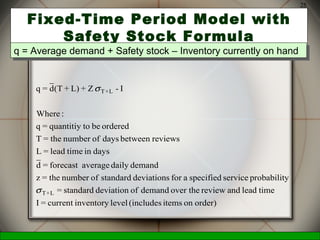
McGraw-Hill/Irwin © 2006 The McGraw-Hill Companies, Inc., All Rights Reserved.
1
Omer MaroofOmer Maroof
MBA 4MBA 4thth
SemesterSemester
Enrollment no:110130Enrollment no:110130
Inventory managementInventory management
decisionsdecisions
McGraw-Hill/Irwin © 2006 The McGraw-Hill Companies, Inc., All Rights Reserved.
2
 Inventory System Defined
 Inventory Costs
 Independent vs. Dependent Demand
 Single-Period Inventory Model
 Multi-Period Inventory Models: Basic
Fixed-Order Quantity Models
 Multi-Period Inventory Models: Basic
Fixed-Time Period Model
 Miscellaneous Systems and Issues
OBJECTIVES
McGraw-Hill/Irwin © 2006 The McGraw-Hill Companies, Inc., All Rights Reserved.
3
Inventory Management
1. DEFINITION
 Inventory in business refers to merchandize held for
sale in ordinary course of business.
 It includes materials and supplies that are consumed
in production .
 It refers to Current Assets.
 It is different from Fixed Assets.
2. Contents of Inventory
 Raw materials.
 Components
 Work in process
 Finished goods
 Consumable
 Machine spares
 Tools, Jigs & Fixtures
McGraw-Hill/Irwin © 2006 The McGraw-Hill Companies, Inc., All Rights Reserved.
4
Inventory System
 Inventory is the stock of any item or
resource used in an organization and
can include: raw materials, finished
products, component parts, supplies,
and work-in-process
 An inventory system is the set of
policies and controls that monitor levels
of inventory and determines what levels
should be maintained, when stock
should be replenished, and how large
orders should be
McGraw-Hill/Irwin © 2006 The McGraw-Hill Companies, Inc., All Rights Reserved.
5
Purposes of Inventory
 To ”decouple” or separate various parts
of the production process
 To provide a stock of goods that will
provide a “selection” for customers
 To take advantage of quantity discounts
 To hedge against inflation and upward
price changes
McGraw-Hill/Irwin © 2006 The McGraw-Hill Companies, Inc., All Rights Reserved.
6
Purposes of Inventory
1. To maintain independence of
operations
2. To meet variation in product demand
3. To allow flexibility in production
scheduling
4. To provide a safeguard for variation in
raw material delivery time
McGraw-Hill/Irwin © 2006 The McGraw-Hill Companies, Inc., All Rights Reserved.
7
Inventory
Process
stage
Demand
Type
Number
& Value
Other
Raw Material
WIP & Finished
Goods
Independent
Dependent
A Items
B Items
C Items
Maintenance
Dependent
Operating
Inventory Classifications
McGraw-Hill/Irwin © 2006 The McGraw-Hill Companies, Inc., All Rights Reserved.
9
SELECTIVE INVENTORY CONTROL
Selective inventory control is defined as process of
classifying items into different categories and thereby
directing appropriate attention to the materials.
It is based on the principle of ‘Vital few and trivial many’
made by Pareto.
CLASSIFICATION
1. A-B-C technique
2. V-E-D classification
3. H-M-L ’’
4. F-S-N ’’
5. S-D-E ’’
6. S-O-S ’’
7. G-O-L-F ’’
8. X-Y-Z ’’ 9
McGraw-Hill/Irwin © 2006 The McGraw-Hill Companies, Inc., All Rights Reserved.
10
Inventory Costs
 Holding (or carrying) costs
– Costs for storage, handling,
insurance, etc
 Setup (or production change) costs
– Costs for arranging specific
equipment setups, etc
 Ordering costs
– Costs of someone placing an order,
etc
 Shortage costs
– Costs of canceling an order, etc
McGraw-Hill/Irwin © 2006 The McGraw-Hill Companies, Inc., All Rights Reserved.
11
E(1
)
Independent vs. Dependent
Demand
Independent Demand (Demand for the final end-
product or demand not related to other items)
Dependent
Demand
(Derived demand
items for
component
parts,
subassemblies,
raw materials,
etc)
Finished
product
Component parts
McGraw-Hill/Irwin © 2006 The McGraw-Hill Companies, Inc., All Rights Reserved.
12
Inventory Systems
 Single-Period Inventory Model
– One time purchasing decision (Example:
vendor selling t-shirts at a football game)
– Seeks to balance the costs of inventory
overstock and under stock
 Multi-Period Inventory Models
– Fixed-Order Quantity Models
 Event triggered (Example: running out of
stock)
– Fixed-Time Period Models
 Time triggered (Example: Monthly sales call
by sales representative)
McGraw-Hill/Irwin © 2006 The McGraw-Hill Companies, Inc., All Rights Reserved.
13
Single-Period Inventory
Model
uo
u
CC
C
P
+
≤
soldbeunit willy that theProbabilit
estimatedunderdemandofunitperCostC
estimatedoverdemandofunitperCostC
:Where
u
o
=
=
=
P
This model states that we
should continue to increase
the size of the inventory so
long as the probability of
selling the last unit added is
equal to or greater than the
ratio of: Cu/Co+Cu
This model states that we
should continue to increase
the size of the inventory so
long as the probability of
selling the last unit added is
equal to or greater than the
ratio of: Cu/Co+Cu
McGraw-Hill/Irwin © 2006 The McGraw-Hill Companies, Inc., All Rights Reserved.
14
Single Period Model
Example
 Our college basketball team is playing in a
tournament game this weekend. Based on our
past experience we sell on average 2,400 shirts
with a standard deviation of 350. We make $10 on
every shirt we sell at the game, but lose $5 on
every shirt not sold. How many shirts should we
make for the game?
Cu = $10 and Co = $5; P ≤ $10 / ($10 + $5) = .667
Z.667 = .432 (use NORMSDIST(.667) or Appendix E)
therefore we need 2,400 + .432(350) = 2,551 shirts
McGraw-Hill/Irwin © 2006 The McGraw-Hill Companies, Inc., All Rights Reserved.
15
Multi-Period Models:
Fixed-Order Quantity Model
Model Assumptions (Part 1)
 Demand for the product is constant
and uniform throughout the period
 Lead time (time from ordering to
receipt) is constant
 Price per unit of product is constant
McGraw-Hill/Irwin © 2006 The McGraw-Hill Companies, Inc., All Rights Reserved.
16
Multi-Period Models:
Fixed-Order Quantity Model Model
Assumptions (Part 2)
 Inventory holding cost is based on
average inventory
 Ordering or setup costs are constant
 All demands for the product will be
satisfied (No back orders are allowed)
McGraw-Hill/Irwin © 2006 The McGraw-Hill Companies, Inc., All Rights Reserved.
17
Basic Fixed-Order Quantity Model
and Reorder Point Behavior
R = Reorder point
Q = Economic order quantity
L = Lead time
L L
Q QQ
R
Time
Number
of units
on hand
1. You receive an order quantity Q.
2. Your start using
them up over time. 3. When you reach down to
a level of inventory of R,
you place your next Q
sized order.
4. The cycle then repeats.
McGraw-Hill/Irwin © 2006 The McGraw-Hill Companies, Inc., All Rights Reserved.
18
Cost Minimization Goal
Ordering Costs
Holding
Costs
Order Quantity (Q)
C
O
S
T
Annual Cost of
Items (DC)
Total Cost
QOPT
By adding the item, holding, and ordering costs
together, we determine the total cost curve, which in
turn is used to find the Qopt inventory order point that
minimizes total costs
By adding the item, holding, and ordering costs
together, we determine the total cost curve, which in
turn is used to find the Qopt inventory order point that
minimizes total costs
McGraw-Hill/Irwin © 2006 The McGraw-Hill Companies, Inc., All Rights Reserved.
19
Basic Fixed-Order Quantity
(EOQ) Model Formula
H
2
Q
+S
Q
D
+DC=TC
Total
Annual =
Cost
Annual
Purchase
Cost
Annual
Ordering
Cost
Annual
Holding
Cost
+ +
TC=Total annual
cost
D =Demand
C =Cost per unit
Q =Order quantity
S =Cost of placing
an order or setup
cost
R =Reorder point
L =Lead time
H=Annual holding
and storage cost
per unit of inventory
TC=Total annual
cost
D =Demand
C =Cost per unit
Q =Order quantity
S =Cost of placing
an order or setup
cost
R =Reorder point
L =Lead time
H=Annual holding
and storage cost
per unit of inventory
McGraw-Hill/Irwin © 2006 The McGraw-Hill Companies, Inc., All Rights Reserved.
20
Deriving the EOQ
Using calculus, we take the first derivative of
the total cost function with respect to Q, and
set the derivative (slope) equal to zero,
solving for the optimized (cost minimized)
value of Qopt
Using calculus, we take the first derivative of
the total cost function with respect to Q, and
set the derivative (slope) equal to zero,
solving for the optimized (cost minimized)
value of Qopt
Q =
2DS
H
=
2(Annual Demand)(Order or Setup Cost)
Annual Holding CostOPT
Reorder point, R = d L
_
d = average daily demand (constant)
L = Lead time (constant)
_
We also need a
reorder point to
tell us when to
place an order
We also need a
reorder point to
tell us when to
place an order
McGraw-Hill/Irwin © 2006 The McGraw-Hill Companies, Inc., All Rights Reserved.
21
EOQ Example (1) Problem
Data
Annual Demand = 1,000 units
Days per year considered in average
daily demand = 365
Cost to place an order = $10
Holding cost per unit per year = $2.50
Lead time = 7 days
Cost per unit = $15
Given the information below, what are the EOQ and
reorder point?
Given the information below, what are the EOQ and
reorder point?
McGraw-Hill/Irwin © 2006 The McGraw-Hill Companies, Inc., All Rights Reserved.
22
EOQ Example (1) Solution
Q =
2DS
H
=
2(1,000 )(10)
2.50
= 89.443 units orOPT 90 units
d =
1,000 units / year
365 days / year
= 2.74 units / day
Reorder point, R = d L = 2.74units / day (7days) = 19.18 or
_
20 units
In summary, you place an optimal order of 90 units. In
the course of using the units to meet demand, when
you only have 20 units left, place the next order of 90
units.
In summary, you place an optimal order of 90 units. In
the course of using the units to meet demand, when
you only have 20 units left, place the next order of 90
units.
McGraw-Hill/Irwin © 2006 The McGraw-Hill Companies, Inc., All Rights Reserved.
23
EOQ Example (2) Problem
Data
Annual Demand = 10,000 units
Days per year considered in average daily
demand = 365
Cost to place an order = $10
Holding cost per unit per year = 10% of cost
per unit
Lead time = 10 days
Cost per unit = $15
Determine the economic order quantity
and the reorder point given the following…
Determine the economic order quantity
and the reorder point given the following…
McGraw-Hill/Irwin © 2006 The McGraw-Hill Companies, Inc., All Rights Reserved.
24
EOQ Example (2) Solution
Q =
2DS
H
=
2(10,000 )(10)
1.50
= 365.148 units, orOPT 366 units
d =
10,000 units / year
365 days / year
= 27.397 units / day
R = d L = 27.397 units / day (10 days) = 273.97 or
_
274 units
Place an order for 366 units. When in the course of
using the inventory you are left with only 274 units,
place the next order of 366 units.
Place an order for 366 units. When in the course of
using the inventory you are left with only 274 units,
place the next order of 366 units.
McGraw-Hill/Irwin © 2006 The McGraw-Hill Companies, Inc., All Rights Reserved.
25
Fixed-Time Period Model with
Safety Stock Formula
order)onitems(includeslevelinventorycurrent=I
timeleadandreviewover thedemandofdeviationstandard=
yprobabilitservicespecifiedafordeviationsstandardofnumberthe=z
demanddailyaverageforecast=d
daysintimelead=L
reviewsbetweendaysofnumberthe=T
orderedbetoquantitiy=q
:Where
I-Z+L)+(Td=q
L+T
L+T
σ
σ
q = Average demand + Safety stock – Inventory currently on handq = Average demand + Safety stock – Inventory currently on hand
McGraw-Hill/Irwin © 2006 The McGraw-Hill Companies, Inc., All Rights Reserved.
26
Multi-Period Models: Fixed-Time Period
Model:
Determining the Value of σT+L
( )σ σ
σ
σ σ
T+L d
i 1
T+L
d
T+L d
2
=
Since each day is independent and is constant,
= (T+ L)
i
2
=
∑
 The standard deviation of a sequence
of random events equals the square
root of the sum of the variances
McGraw-Hill/Irwin © 2006 The McGraw-Hill Companies, Inc., All Rights Reserved.
27
Example of the Fixed-Time Period
Model
Average daily demand for a product is
20 units. The review period is 30 days,
and lead time is 10 days. Management
has set a policy of satisfying 96 percent
of demand from items in stock. At the
beginning of the review period there are
200 units in inventory. The daily
demand standard deviation is 4 units.
Given the information below, how many units
should be ordered?
Given the information below, how many units
should be ordered?
McGraw-Hill/Irwin © 2006 The McGraw-Hill Companies, Inc., All Rights Reserved.
28
Example of the Fixed-Time
Period Model: Solution (Part 1)
( )( )σ σT+L d
2 2
= (T + L) = 30 +10 4 = 25.298( )( )σ σT+L d
2 2
= (T + L) = 30 +10 4 = 25.298
The value for “z” is found by using the Excel
NORMSINV function, or as we will do here, using
Appendix D. By adding 0.5 to all the values in
Appendix D and finding the value in the table that
comes closest to the service probability, the “z”
value can be read by adding the column heading
label to the row label.
So, by adding 0.5 to the value from Appendix D of 0.4599,
we have a probability of 0.9599, which is given by a z = 1.75
So, by adding 0.5 to the value from Appendix D of 0.4599,
we have a probability of 0.9599, which is given by a z = 1.75
McGraw-Hill/Irwin © 2006 The McGraw-Hill Companies, Inc., All Rights Reserved.
29
Example of the Fixed-Time
Period Model: Solution (Part 2)
or644.272,=200-44.272800=q
200-298)(1.75)(25.+10)+20(30=q
I-Z+L)+(Td=q L+T
units645+
σ
So, to satisfy 96 percent of the demand,
you should place an order of 645 units at
this review period
So, to satisfy 96 percent of the demand,
you should place an order of 645 units at
this review period
McGraw-Hill/Irwin © 2006 The McGraw-Hill Companies, Inc., All Rights Reserved.
30
Price-Break Model Formula
CostHoldingAnnual
Cost)SetuporderDemand)(Or2(Annual
=
iC
2DS
=QOPT
Based on the same assumptions as the EOQ model,
the price-break model has a similar Qopt formula:
i = percentage of unit cost attributed to carrying inventory
C = cost per unit
Since “C” changes for each price-break, the formula
above will have to be used with each price-break cost
value
McGraw-Hill/Irwin © 2006 The McGraw-Hill Companies, Inc., All Rights Reserved.
31
Price-Break Example Problem Data
(Part 1)
A company has a chance to reduce their inventory
ordering costs by placing larger quantity orders using
the price-break order quantity schedule below. What
should their optimal order quantity be if this company
purchases this single inventory item with an e-mail
ordering cost of $4, a carrying cost rate of 2% of the
inventory cost of the item, and an annual demand of
10,000 units?
Order Quantity(units) Price/unit($)
0 to 2,499 $1.20
2,500 to 3,999 1.00
4,000 or more .98
McGraw-Hill/Irwin © 2006 The McGraw-Hill Companies, Inc., All Rights Reserved.
32
Price-Break Example Solution
(Part 2)
units1,826=
0.02(1.20)
4)2(10,000)(
=
iC
2DS
=QOPT
Annual Demand (D)= 10,000 units
Cost to place an order (S)= $4
First, plug data into formula for each price-break value of “C”
units2,000=
0.02(1.00)
4)2(10,000)(
=
iC
2DS
=QOPT
units2,020=
0.02(0.98)
4)2(10,000)(
=
iC
2DS
=QOPT
Carrying cost % of total cost (i)= 2%
Cost per unit (C) = $1.20, $1.00, $0.98
Interval from 0 to 2499, the
Qopt value is feasible
Interval from 2500-3999, the
Qopt value is not feasible
Interval from 4000 & more, the
Qopt value is not feasible
Next, determine if the computed Qopt values are feasible or not
McGraw-Hill/Irwin © 2006 The McGraw-Hill Companies, Inc., All Rights Reserved.
33
Price-Break Example Solution
(Part 3)
Since the feasible solution occurred in the first price-
break, it means that all the other true Qopt values occur
at the beginnings of each price-break interval. Why?
Since the feasible solution occurred in the first price-
break, it means that all the other true Qopt values occur
at the beginnings of each price-break interval. Why?
0 1826 2500 4000 Order Quantity
Total
annual
costs
So the candidates
for the price-
breaks are 1826,
2500, and 4000
units
So the candidates
for the price-
breaks are 1826,
2500, and 4000
units
Because the total annual cost function is
a “u” shaped function
Because the total annual cost function is
a “u” shaped function
McGraw-Hill/Irwin © 2006 The McGraw-Hill Companies, Inc., All Rights Reserved.
34
Price-Break Example Solution (Part
4)
iC
2
Q
+S
Q
D
+DC=TC
Next, we plug the true Qopt values into the total cost
annual cost function to determine the total cost under
each price-break
Next, we plug the true Qopt values into the total cost
annual cost function to determine the total cost under
each price-break
TC(0-2499)=(10000*1.20)+(10000/1826)*4+(1826/2)(0.02*1.20)
= $12,043.82
TC(2500-3999)= $10,041
TC(4000&more)= $9,949.20
TC(0-2499)=(10000*1.20)+(10000/1826)*4+(1826/2)(0.02*1.20)
= $12,043.82
TC(2500-3999)= $10,041
TC(4000&more)= $9,949.20
Finally, we select the least costly Qopt, which is this
problem occurs in the 4000 & more interval. In
summary, our optimal order quantity is 4000 units
Finally, we select the least costly Qopt, which is this
problem occurs in the 4000 & more interval. In
summary, our optimal order quantity is 4000 units
McGraw-Hill/Irwin © 2006 The McGraw-Hill Companies, Inc., All Rights Reserved.
35
Maximum Inventory Level, M
Miscellaneous Systems:
Optional Replenishment System
M
Actual Inventory Level, I
q = M - I
I
Q = minimum acceptable order quantity
If q > Q, order q, otherwise do not order any.
McGraw-Hill/Irwin © 2006 The McGraw-Hill Companies, Inc., All Rights Reserved.
36
Miscellaneous Systems:
Bin Systems
Two-Bin System
Full Empty
Order One Bin of
Inventory
One-Bin System
Periodic Check
Order Enough to
Refill Bin
McGraw-Hill/Irwin © 2006 The McGraw-Hill Companies, Inc., All Rights Reserved.
37
ABC Classification System
 Items kept in inventory are not of equal
importance in terms of:
– dollars invested
– profit potential
– sales or usage volume
– stock-out penalties
0
30
60
30
60
A
B
C
% of
$ Value
% of
Use
So, identify inventory items based on percentage of total
dollar value, where “A” items are roughly top 15 %, “B”
items as next 35 %, and the lower 65% are the “C” items
McGraw-Hill/Irwin © 2006 The McGraw-Hill Companies, Inc., All Rights Reserved.
38
Inventory Accuracy and Cycle
Counting
 Inventory accuracy refers to how
well the inventory records agree
with physical count
 Cycle Counting is a physical
inventory-taking technique in which
inventory is counted on a frequent
basis rather than once or twice a
year
McGraw-Hill/Irwin © 2006 The McGraw-Hill Companies, Inc., All Rights Reserved.
39

Inventory management

  • 1.
    McGraw-Hill/Irwin © 2006The McGraw-Hill Companies, Inc., All Rights Reserved. 1 Omer MaroofOmer Maroof MBA 4MBA 4thth SemesterSemester Enrollment no:110130Enrollment no:110130 Inventory managementInventory management decisionsdecisions
  • 2.
    McGraw-Hill/Irwin © 2006The McGraw-Hill Companies, Inc., All Rights Reserved. 2  Inventory System Defined  Inventory Costs  Independent vs. Dependent Demand  Single-Period Inventory Model  Multi-Period Inventory Models: Basic Fixed-Order Quantity Models  Multi-Period Inventory Models: Basic Fixed-Time Period Model  Miscellaneous Systems and Issues OBJECTIVES
  • 3.
    McGraw-Hill/Irwin © 2006The McGraw-Hill Companies, Inc., All Rights Reserved. 3 Inventory Management 1. DEFINITION  Inventory in business refers to merchandize held for sale in ordinary course of business.  It includes materials and supplies that are consumed in production .  It refers to Current Assets.  It is different from Fixed Assets. 2. Contents of Inventory  Raw materials.  Components  Work in process  Finished goods  Consumable  Machine spares  Tools, Jigs & Fixtures
  • 4.
    McGraw-Hill/Irwin © 2006The McGraw-Hill Companies, Inc., All Rights Reserved. 4 Inventory System  Inventory is the stock of any item or resource used in an organization and can include: raw materials, finished products, component parts, supplies, and work-in-process  An inventory system is the set of policies and controls that monitor levels of inventory and determines what levels should be maintained, when stock should be replenished, and how large orders should be
  • 5.
    McGraw-Hill/Irwin © 2006The McGraw-Hill Companies, Inc., All Rights Reserved. 5 Purposes of Inventory  To ”decouple” or separate various parts of the production process  To provide a stock of goods that will provide a “selection” for customers  To take advantage of quantity discounts  To hedge against inflation and upward price changes
  • 6.
    McGraw-Hill/Irwin © 2006The McGraw-Hill Companies, Inc., All Rights Reserved. 6 Purposes of Inventory 1. To maintain independence of operations 2. To meet variation in product demand 3. To allow flexibility in production scheduling 4. To provide a safeguard for variation in raw material delivery time
  • 7.
    McGraw-Hill/Irwin © 2006The McGraw-Hill Companies, Inc., All Rights Reserved. 7 Inventory Process stage Demand Type Number & Value Other Raw Material WIP & Finished Goods Independent Dependent A Items B Items C Items Maintenance Dependent Operating Inventory Classifications
  • 8.
    McGraw-Hill/Irwin © 2006The McGraw-Hill Companies, Inc., All Rights Reserved. 9 SELECTIVE INVENTORY CONTROL Selective inventory control is defined as process of classifying items into different categories and thereby directing appropriate attention to the materials. It is based on the principle of ‘Vital few and trivial many’ made by Pareto. CLASSIFICATION 1. A-B-C technique 2. V-E-D classification 3. H-M-L ’’ 4. F-S-N ’’ 5. S-D-E ’’ 6. S-O-S ’’ 7. G-O-L-F ’’ 8. X-Y-Z ’’ 9
  • 9.
    McGraw-Hill/Irwin © 2006The McGraw-Hill Companies, Inc., All Rights Reserved. 10 Inventory Costs  Holding (or carrying) costs – Costs for storage, handling, insurance, etc  Setup (or production change) costs – Costs for arranging specific equipment setups, etc  Ordering costs – Costs of someone placing an order, etc  Shortage costs – Costs of canceling an order, etc
  • 10.
    McGraw-Hill/Irwin © 2006The McGraw-Hill Companies, Inc., All Rights Reserved. 11 E(1 ) Independent vs. Dependent Demand Independent Demand (Demand for the final end- product or demand not related to other items) Dependent Demand (Derived demand items for component parts, subassemblies, raw materials, etc) Finished product Component parts
  • 11.
    McGraw-Hill/Irwin © 2006The McGraw-Hill Companies, Inc., All Rights Reserved. 12 Inventory Systems  Single-Period Inventory Model – One time purchasing decision (Example: vendor selling t-shirts at a football game) – Seeks to balance the costs of inventory overstock and under stock  Multi-Period Inventory Models – Fixed-Order Quantity Models  Event triggered (Example: running out of stock) – Fixed-Time Period Models  Time triggered (Example: Monthly sales call by sales representative)
  • 12.
    McGraw-Hill/Irwin © 2006The McGraw-Hill Companies, Inc., All Rights Reserved. 13 Single-Period Inventory Model uo u CC C P + ≤ soldbeunit willy that theProbabilit estimatedunderdemandofunitperCostC estimatedoverdemandofunitperCostC :Where u o = = = P This model states that we should continue to increase the size of the inventory so long as the probability of selling the last unit added is equal to or greater than the ratio of: Cu/Co+Cu This model states that we should continue to increase the size of the inventory so long as the probability of selling the last unit added is equal to or greater than the ratio of: Cu/Co+Cu
  • 13.
    McGraw-Hill/Irwin © 2006The McGraw-Hill Companies, Inc., All Rights Reserved. 14 Single Period Model Example  Our college basketball team is playing in a tournament game this weekend. Based on our past experience we sell on average 2,400 shirts with a standard deviation of 350. We make $10 on every shirt we sell at the game, but lose $5 on every shirt not sold. How many shirts should we make for the game? Cu = $10 and Co = $5; P ≤ $10 / ($10 + $5) = .667 Z.667 = .432 (use NORMSDIST(.667) or Appendix E) therefore we need 2,400 + .432(350) = 2,551 shirts
  • 14.
    McGraw-Hill/Irwin © 2006The McGraw-Hill Companies, Inc., All Rights Reserved. 15 Multi-Period Models: Fixed-Order Quantity Model Model Assumptions (Part 1)  Demand for the product is constant and uniform throughout the period  Lead time (time from ordering to receipt) is constant  Price per unit of product is constant
  • 15.
    McGraw-Hill/Irwin © 2006The McGraw-Hill Companies, Inc., All Rights Reserved. 16 Multi-Period Models: Fixed-Order Quantity Model Model Assumptions (Part 2)  Inventory holding cost is based on average inventory  Ordering or setup costs are constant  All demands for the product will be satisfied (No back orders are allowed)
  • 16.
    McGraw-Hill/Irwin © 2006The McGraw-Hill Companies, Inc., All Rights Reserved. 17 Basic Fixed-Order Quantity Model and Reorder Point Behavior R = Reorder point Q = Economic order quantity L = Lead time L L Q QQ R Time Number of units on hand 1. You receive an order quantity Q. 2. Your start using them up over time. 3. When you reach down to a level of inventory of R, you place your next Q sized order. 4. The cycle then repeats.
  • 17.
    McGraw-Hill/Irwin © 2006The McGraw-Hill Companies, Inc., All Rights Reserved. 18 Cost Minimization Goal Ordering Costs Holding Costs Order Quantity (Q) C O S T Annual Cost of Items (DC) Total Cost QOPT By adding the item, holding, and ordering costs together, we determine the total cost curve, which in turn is used to find the Qopt inventory order point that minimizes total costs By adding the item, holding, and ordering costs together, we determine the total cost curve, which in turn is used to find the Qopt inventory order point that minimizes total costs
  • 18.
    McGraw-Hill/Irwin © 2006The McGraw-Hill Companies, Inc., All Rights Reserved. 19 Basic Fixed-Order Quantity (EOQ) Model Formula H 2 Q +S Q D +DC=TC Total Annual = Cost Annual Purchase Cost Annual Ordering Cost Annual Holding Cost + + TC=Total annual cost D =Demand C =Cost per unit Q =Order quantity S =Cost of placing an order or setup cost R =Reorder point L =Lead time H=Annual holding and storage cost per unit of inventory TC=Total annual cost D =Demand C =Cost per unit Q =Order quantity S =Cost of placing an order or setup cost R =Reorder point L =Lead time H=Annual holding and storage cost per unit of inventory
  • 19.
    McGraw-Hill/Irwin © 2006The McGraw-Hill Companies, Inc., All Rights Reserved. 20 Deriving the EOQ Using calculus, we take the first derivative of the total cost function with respect to Q, and set the derivative (slope) equal to zero, solving for the optimized (cost minimized) value of Qopt Using calculus, we take the first derivative of the total cost function with respect to Q, and set the derivative (slope) equal to zero, solving for the optimized (cost minimized) value of Qopt Q = 2DS H = 2(Annual Demand)(Order or Setup Cost) Annual Holding CostOPT Reorder point, R = d L _ d = average daily demand (constant) L = Lead time (constant) _ We also need a reorder point to tell us when to place an order We also need a reorder point to tell us when to place an order
  • 20.
    McGraw-Hill/Irwin © 2006The McGraw-Hill Companies, Inc., All Rights Reserved. 21 EOQ Example (1) Problem Data Annual Demand = 1,000 units Days per year considered in average daily demand = 365 Cost to place an order = $10 Holding cost per unit per year = $2.50 Lead time = 7 days Cost per unit = $15 Given the information below, what are the EOQ and reorder point? Given the information below, what are the EOQ and reorder point?
  • 21.
    McGraw-Hill/Irwin © 2006The McGraw-Hill Companies, Inc., All Rights Reserved. 22 EOQ Example (1) Solution Q = 2DS H = 2(1,000 )(10) 2.50 = 89.443 units orOPT 90 units d = 1,000 units / year 365 days / year = 2.74 units / day Reorder point, R = d L = 2.74units / day (7days) = 19.18 or _ 20 units In summary, you place an optimal order of 90 units. In the course of using the units to meet demand, when you only have 20 units left, place the next order of 90 units. In summary, you place an optimal order of 90 units. In the course of using the units to meet demand, when you only have 20 units left, place the next order of 90 units.
  • 22.
    McGraw-Hill/Irwin © 2006The McGraw-Hill Companies, Inc., All Rights Reserved. 23 EOQ Example (2) Problem Data Annual Demand = 10,000 units Days per year considered in average daily demand = 365 Cost to place an order = $10 Holding cost per unit per year = 10% of cost per unit Lead time = 10 days Cost per unit = $15 Determine the economic order quantity and the reorder point given the following… Determine the economic order quantity and the reorder point given the following…
  • 23.
    McGraw-Hill/Irwin © 2006The McGraw-Hill Companies, Inc., All Rights Reserved. 24 EOQ Example (2) Solution Q = 2DS H = 2(10,000 )(10) 1.50 = 365.148 units, orOPT 366 units d = 10,000 units / year 365 days / year = 27.397 units / day R = d L = 27.397 units / day (10 days) = 273.97 or _ 274 units Place an order for 366 units. When in the course of using the inventory you are left with only 274 units, place the next order of 366 units. Place an order for 366 units. When in the course of using the inventory you are left with only 274 units, place the next order of 366 units.
  • 24.
    McGraw-Hill/Irwin © 2006The McGraw-Hill Companies, Inc., All Rights Reserved. 25 Fixed-Time Period Model with Safety Stock Formula order)onitems(includeslevelinventorycurrent=I timeleadandreviewover thedemandofdeviationstandard= yprobabilitservicespecifiedafordeviationsstandardofnumberthe=z demanddailyaverageforecast=d daysintimelead=L reviewsbetweendaysofnumberthe=T orderedbetoquantitiy=q :Where I-Z+L)+(Td=q L+T L+T σ σ q = Average demand + Safety stock – Inventory currently on handq = Average demand + Safety stock – Inventory currently on hand
  • 25.
    McGraw-Hill/Irwin © 2006The McGraw-Hill Companies, Inc., All Rights Reserved. 26 Multi-Period Models: Fixed-Time Period Model: Determining the Value of σT+L ( )σ σ σ σ σ T+L d i 1 T+L d T+L d 2 = Since each day is independent and is constant, = (T+ L) i 2 = ∑  The standard deviation of a sequence of random events equals the square root of the sum of the variances
  • 26.
    McGraw-Hill/Irwin © 2006The McGraw-Hill Companies, Inc., All Rights Reserved. 27 Example of the Fixed-Time Period Model Average daily demand for a product is 20 units. The review period is 30 days, and lead time is 10 days. Management has set a policy of satisfying 96 percent of demand from items in stock. At the beginning of the review period there are 200 units in inventory. The daily demand standard deviation is 4 units. Given the information below, how many units should be ordered? Given the information below, how many units should be ordered?
  • 27.
    McGraw-Hill/Irwin © 2006The McGraw-Hill Companies, Inc., All Rights Reserved. 28 Example of the Fixed-Time Period Model: Solution (Part 1) ( )( )σ σT+L d 2 2 = (T + L) = 30 +10 4 = 25.298( )( )σ σT+L d 2 2 = (T + L) = 30 +10 4 = 25.298 The value for “z” is found by using the Excel NORMSINV function, or as we will do here, using Appendix D. By adding 0.5 to all the values in Appendix D and finding the value in the table that comes closest to the service probability, the “z” value can be read by adding the column heading label to the row label. The value for “z” is found by using the Excel NORMSINV function, or as we will do here, using Appendix D. By adding 0.5 to all the values in Appendix D and finding the value in the table that comes closest to the service probability, the “z” value can be read by adding the column heading label to the row label. So, by adding 0.5 to the value from Appendix D of 0.4599, we have a probability of 0.9599, which is given by a z = 1.75 So, by adding 0.5 to the value from Appendix D of 0.4599, we have a probability of 0.9599, which is given by a z = 1.75
  • 28.
    McGraw-Hill/Irwin © 2006The McGraw-Hill Companies, Inc., All Rights Reserved. 29 Example of the Fixed-Time Period Model: Solution (Part 2) or644.272,=200-44.272800=q 200-298)(1.75)(25.+10)+20(30=q I-Z+L)+(Td=q L+T units645+ σ So, to satisfy 96 percent of the demand, you should place an order of 645 units at this review period So, to satisfy 96 percent of the demand, you should place an order of 645 units at this review period
  • 29.
    McGraw-Hill/Irwin © 2006The McGraw-Hill Companies, Inc., All Rights Reserved. 30 Price-Break Model Formula CostHoldingAnnual Cost)SetuporderDemand)(Or2(Annual = iC 2DS =QOPT Based on the same assumptions as the EOQ model, the price-break model has a similar Qopt formula: i = percentage of unit cost attributed to carrying inventory C = cost per unit Since “C” changes for each price-break, the formula above will have to be used with each price-break cost value
  • 30.
    McGraw-Hill/Irwin © 2006The McGraw-Hill Companies, Inc., All Rights Reserved. 31 Price-Break Example Problem Data (Part 1) A company has a chance to reduce their inventory ordering costs by placing larger quantity orders using the price-break order quantity schedule below. What should their optimal order quantity be if this company purchases this single inventory item with an e-mail ordering cost of $4, a carrying cost rate of 2% of the inventory cost of the item, and an annual demand of 10,000 units? A company has a chance to reduce their inventory ordering costs by placing larger quantity orders using the price-break order quantity schedule below. What should their optimal order quantity be if this company purchases this single inventory item with an e-mail ordering cost of $4, a carrying cost rate of 2% of the inventory cost of the item, and an annual demand of 10,000 units? Order Quantity(units) Price/unit($) 0 to 2,499 $1.20 2,500 to 3,999 1.00 4,000 or more .98
  • 31.
    McGraw-Hill/Irwin © 2006The McGraw-Hill Companies, Inc., All Rights Reserved. 32 Price-Break Example Solution (Part 2) units1,826= 0.02(1.20) 4)2(10,000)( = iC 2DS =QOPT Annual Demand (D)= 10,000 units Cost to place an order (S)= $4 First, plug data into formula for each price-break value of “C” units2,000= 0.02(1.00) 4)2(10,000)( = iC 2DS =QOPT units2,020= 0.02(0.98) 4)2(10,000)( = iC 2DS =QOPT Carrying cost % of total cost (i)= 2% Cost per unit (C) = $1.20, $1.00, $0.98 Interval from 0 to 2499, the Qopt value is feasible Interval from 2500-3999, the Qopt value is not feasible Interval from 4000 & more, the Qopt value is not feasible Next, determine if the computed Qopt values are feasible or not
  • 32.
    McGraw-Hill/Irwin © 2006The McGraw-Hill Companies, Inc., All Rights Reserved. 33 Price-Break Example Solution (Part 3) Since the feasible solution occurred in the first price- break, it means that all the other true Qopt values occur at the beginnings of each price-break interval. Why? Since the feasible solution occurred in the first price- break, it means that all the other true Qopt values occur at the beginnings of each price-break interval. Why? 0 1826 2500 4000 Order Quantity Total annual costs So the candidates for the price- breaks are 1826, 2500, and 4000 units So the candidates for the price- breaks are 1826, 2500, and 4000 units Because the total annual cost function is a “u” shaped function Because the total annual cost function is a “u” shaped function
  • 33.
    McGraw-Hill/Irwin © 2006The McGraw-Hill Companies, Inc., All Rights Reserved. 34 Price-Break Example Solution (Part 4) iC 2 Q +S Q D +DC=TC Next, we plug the true Qopt values into the total cost annual cost function to determine the total cost under each price-break Next, we plug the true Qopt values into the total cost annual cost function to determine the total cost under each price-break TC(0-2499)=(10000*1.20)+(10000/1826)*4+(1826/2)(0.02*1.20) = $12,043.82 TC(2500-3999)= $10,041 TC(4000&more)= $9,949.20 TC(0-2499)=(10000*1.20)+(10000/1826)*4+(1826/2)(0.02*1.20) = $12,043.82 TC(2500-3999)= $10,041 TC(4000&more)= $9,949.20 Finally, we select the least costly Qopt, which is this problem occurs in the 4000 & more interval. In summary, our optimal order quantity is 4000 units Finally, we select the least costly Qopt, which is this problem occurs in the 4000 & more interval. In summary, our optimal order quantity is 4000 units
  • 34.
    McGraw-Hill/Irwin © 2006The McGraw-Hill Companies, Inc., All Rights Reserved. 35 Maximum Inventory Level, M Miscellaneous Systems: Optional Replenishment System M Actual Inventory Level, I q = M - I I Q = minimum acceptable order quantity If q > Q, order q, otherwise do not order any.
  • 35.
    McGraw-Hill/Irwin © 2006The McGraw-Hill Companies, Inc., All Rights Reserved. 36 Miscellaneous Systems: Bin Systems Two-Bin System Full Empty Order One Bin of Inventory One-Bin System Periodic Check Order Enough to Refill Bin
  • 36.
    McGraw-Hill/Irwin © 2006The McGraw-Hill Companies, Inc., All Rights Reserved. 37 ABC Classification System  Items kept in inventory are not of equal importance in terms of: – dollars invested – profit potential – sales or usage volume – stock-out penalties 0 30 60 30 60 A B C % of $ Value % of Use So, identify inventory items based on percentage of total dollar value, where “A” items are roughly top 15 %, “B” items as next 35 %, and the lower 65% are the “C” items
  • 37.
    McGraw-Hill/Irwin © 2006The McGraw-Hill Companies, Inc., All Rights Reserved. 38 Inventory Accuracy and Cycle Counting  Inventory accuracy refers to how well the inventory records agree with physical count  Cycle Counting is a physical inventory-taking technique in which inventory is counted on a frequent basis rather than once or twice a year
  • 38.
    McGraw-Hill/Irwin © 2006The McGraw-Hill Companies, Inc., All Rights Reserved. 39