Download as PDF, PPTX


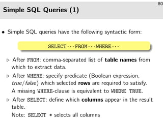
![Renaming Output Columns
89
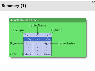
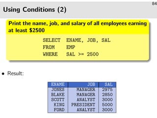
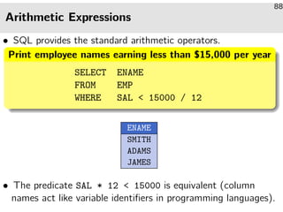
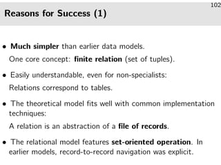
Print the yearly salary of all managers
SELECT ENAME, SAL * 12
FROM EMP
WHERE JOB = ’MANAGER’
ENAME SAL * 12
JONES 35700
BLAKE 34200
CLARK 29400
• To rename the second result column:
SELECT ENAME, SAL * 12 [AS] YEARLY SALARY . . .](https://image.slidesharecdn.com/www-db-160124182847/85/Introduction-to-the-Relational-Model-and-SQL-29-320.jpg)
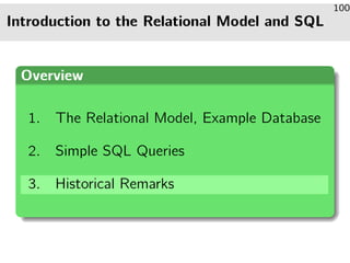
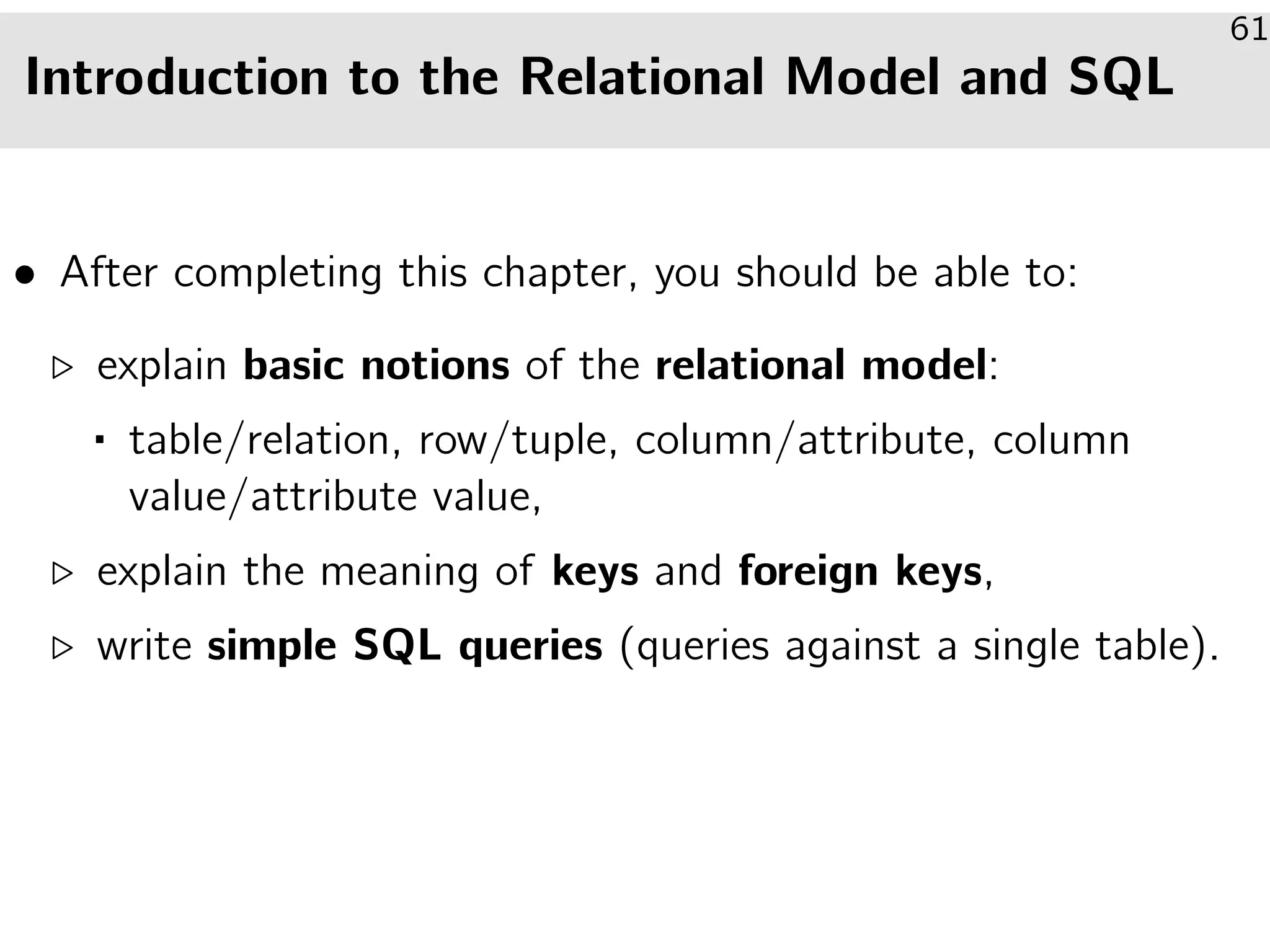
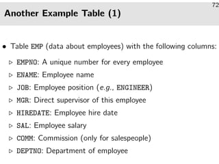
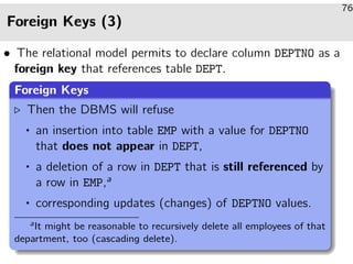
The document introduces the relational model and SQL, explaining concepts such as tables, keys, and basic SQL queries. It outlines the structure of a relational database and details how to write simple SQL commands for data retrieval and manipulation. Historical context is provided, noting the development of the relational model by Edgar F. Codd and its successful implementation in various database systems.


![Spreadsheets[1]](https://cdn.slidesharecdn.com/ss_thumbnails/spreadsheets1-150131022908-conversion-gate01-thumbnail.jpg?width=640&height=640&fit=bounds)