


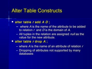

![INSERT operation
Add a new tuple to a table
INSERT
INTO table [ (field [,field] … )]
VALUES (literal[,literal ] …) ;](https://image.slidesharecdn.com/db1lecture4-130314233105-phpapp01/85/Db1-lecture4-16-320.jpg)

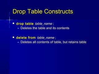
![UPDATE operation
General format
UPDATE table
SET field = scalar-expression
[, field = scalar-expression ] …..
[ WHERE condition ] ;](https://image.slidesharecdn.com/db1lecture4-130314233105-phpapp01/85/Db1-lecture4-18-320.jpg)

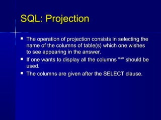
![DELETE operation
Delete all records in a “table” that satisfy a
“condition”
General format
DELETE FROM table [ WHERE condition ] ;](https://image.slidesharecdn.com/db1lecture4-130314233105-phpapp01/85/Db1-lecture4-20-320.jpg)

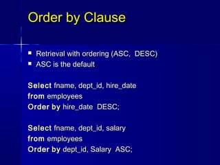
![Interrogation operation
Queries are done by using SELECT command
The result of an SQL query is a relation.
Syntax of the SELECT command
SELECT [DISTINCT ] {* | expr [AS alias], ... }
FROM table [alias], ...
[WHERE { conditions | under conditions} ]
[GROUP BY expr, ...] [HAVING conditions]
[ORDER BY {expr | num}{ASC | DESC }, ...];](https://image.slidesharecdn.com/db1lecture4-130314233105-phpapp01/85/Db1-lecture4-22-320.jpg)
![SELECT command
Syntactical agreements
CAPITAL LETTERS : (SELECT) Enter values exactly as presented.
Italic : column, table. Parameter having to be replaced
by the suitable value.
Alias : Synonym of a name of table or column.
Conditions : Expression having the true or false value.
Under conditions : Expression containing a subquery.
Expr : Column, or calculated attribute (+,-, *, /)
Num : Column number
{} : Ex {ON|OFF}. One of the values separated by "|"
must obligatory be typed in.
[ ] : optional Value.
( ) : the brackets and commas must be type in as
presented.
... : The preceding values can be repeated several
times
_ Underlined : indicate the default value.](https://image.slidesharecdn.com/db1lecture4-130314233105-phpapp01/85/Db1-lecture4-23-320.jpg)


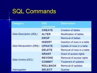
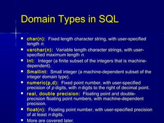
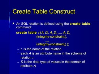
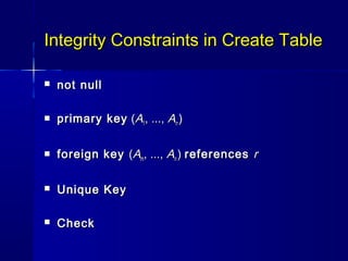
This document provides an introduction to SQL (Structured Query Language). SQL is a language used to define, query, modify, and control relational databases. The document outlines the main SQL commands for data definition (CREATE, ALTER, DROP), data manipulation (INSERT, UPDATE, DELETE), and data control (GRANT, REVOKE). It also discusses SQL data types, integrity constraints, and how to use SELECT statements to query databases using projections, selections, comparisons, logical conditions, and ordering. The FROM clause is introduced as specifying the relations involved in a query.