This document is a physics project final report that introduces the concept of combining higher order vectors and the connection on a manifold. It defines higher order vectors up to arbitrary order using both index and coordinate-free representations. It then investigates how higher order vectors and the connection transform between coordinate systems. Finally, it suggests two ways of combining second and third order vectors with the connection and shows how this naturally introduces the torsion and curvature of the manifold. The report emphasizes developing coordinate-free definitions and discusses potential applications, such as rewriting equations from general relativity by viewing higher order vectors as a new source of matter.
![1 Introduction
The connection is a highly useful geometric object which appears in many areas of physics
and mathematics. It is a idea that will be a familiar to many through its applications in gen-
eral relativity and fluid physics, featuring in both the geodesic deviation and Navier-Stokes
equations[10][12]. In these equations it acts as the covariant or directional derivative, providing
a way of differentiating one vector field along another vector field on a manifold. A seeming
unrelated concept at first is that of a higher order vector, introduced in a paper by Duval which
studied differential operators on manifolds[5]. Their application to systems of ordinary differen-
tial equations was then investigated by Aghasi et al in 2006, yet they remain a rather abstract
concept[1]. Although higher order vectors do not lend themselves to an intuitive introduction,
a natural relationship exists between them and connection. This relationship becomes evident
when each of their transformation laws are calculated. It will be shown that both the connection
and higher order vectors are non-tensorial, that is to say in general they are dependent on the
choice of coordinate basis. With this shared property in mind, it can be asked whether the non-
tensorial nature of the two objects can be exploited in such a way, that they can be combined to
form an overall tensor. Tensors of course do not depend on the choice of basis, a property which
makes them far more useful for constructing physical theories. This project began with nothing
more than the assumption that such tensorial objects should exist, at least when working with
the ‘lowest order,’ higher order vectors. The method then being to take products of the various
non-tensorial objects in such a way that if searching for a vectorial component for example, only
one free contravariant index is left. The transformation properties of this newly constructed
object are then worked out by direct computation, confirming whether or not a true vector has
been built. As far as we are aware, the combination of higher order vectors and the connection
in this way has not been seen before. Up until this point, research has been centred around
second and third order vectors. It is believed however that an inductive definition, describing
how the connection and a vector of arbitrary order can be combined, does exist. This possibility
will be explored in more detail in later sections.
Throughout the project, classical tensor calculus is the primary technique which is used. This is
the manipulation of tensorial and tensor-like objects using index notation. It is a very common
algebraic method which features heavily at undergraduate level, in topics such as general rela-
tivity. One of the main problems with this classical approach is that it requires reference to a
coordinate system, which in turn means the introduction of a metric. From the project’s outset,
the research has been focussed on defining in a coordinate free way, how higher order vectors
can be combined with the connection. At least at low orders, our research has found that from
this viewpoint, the concepts of torsion and curvature are naturally introduced. These are two
physical quantities which play central roles in modern theories of nature. Curvature has long
been considered in general relativity as the ‘source’ of gravity, whereas the possible significance
of torsion was only more recently recognised[12]. Potential areas of application which could ex-
ploit this natural appearance of torsion, are discussed more closely toward the end of the report.
The description of objects and physical laws without reference to a basis is not a new idea. It is
the foundation of a field known as differential geometry, an extremely powerful tool in theoretical
physics. In this language for example, all four of Maxwell’s equations can be reduced to just two,
describing fully relativistically, the electro-magnetic fields in any spacetime[12]. Furthermore,
a classical vector is no longer defined by its transformation properties, but by a set of basic
algebraic rules. It is believed that a coordinate free approach to higher order vectors has not yet
been attempted. As well as the final definitions themselves, the report puts much emphasis on
the process by which the definitions evolve from coordinate, to coordinate free. During research,
a number of tools were developed to do this effectively.
3](https://image.slidesharecdn.com/46491f5f-30bc-4c7a-99ba-d9cbbd913c19-150725210144-lva1-app6891/75/SubmissionCopyAlexanderBooth-3-2048.jpg)
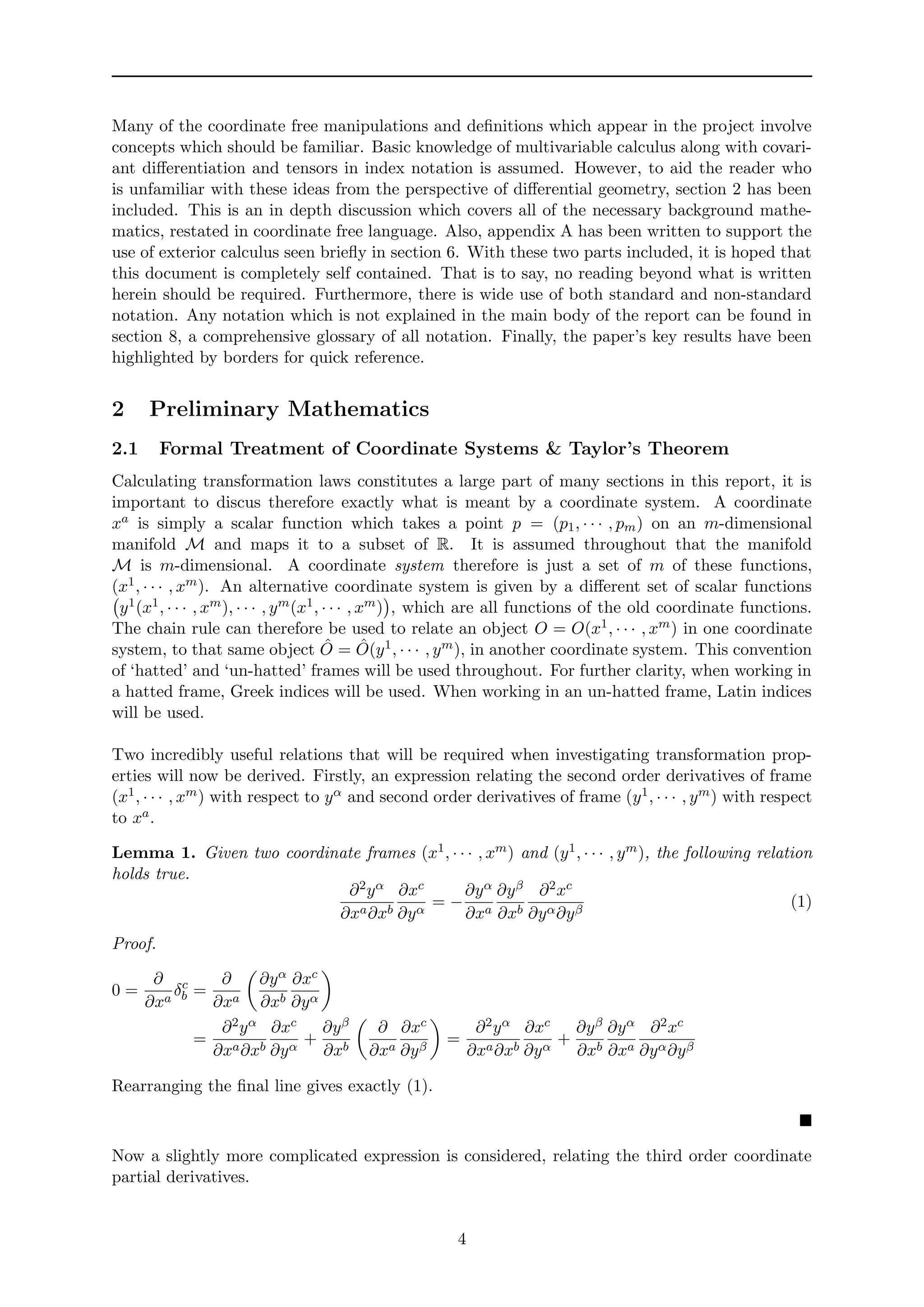
![2.1 Formal Treatment of Coordinate Systems & Taylor’s Theorem
Lemma 2. Given two coordinate frames (x1, · · · , xm) and (y1, · · · , ym), the following relation
holds true.
∂3y
∂xa∂xb∂xc
= −
∂yγ
∂xc
∂y
∂xd
∂2yα
∂xa∂xb
∂2xd
∂yα∂yγ
+
∂y
∂xd
∂yβ
∂xa
∂2yα
∂xb∂xc
∂2xd
∂yα∂yβ
(2)
+
∂y
∂xd
∂yα
∂xb
∂2yβ
∂xa∂xc
∂2xd
∂yα∂yβ
+
∂yγ
∂xc
∂y
∂xd
∂yα
∂xb
∂yβ
∂xa
∂3xd
∂yα∂yβ∂yγ
Proof. The result follows from partially differentiating each side of equation (1). Beginning
with the left hand side.
∂
∂yγ
∂2y
∂xa∂xb
∂xc
∂y
=
∂xd
∂yγ
∂xc
∂y
∂3y
∂xa∂xd∂xb
+
∂2y
∂xa∂xb
∂2xc
∂yγ∂y
Now the right hand side.
∂
∂yγ
−
∂yα
∂xb
∂yβ
∂xa
∂2xc
∂yα∂yβ
= −
∂xd
∂yγ
∂2yα
∂xb∂xd
∂yβ
∂xa
∂2xc
∂yα∂yβ
+
∂xd
∂yγ
∂yα
∂xb
∂2yβ
∂xa∂xd
∂2xc
∂yα∂yβ
+
∂yα
∂xb
∂yβ
∂xa
∂3xc
∂yα∂yβ∂yγ
Rearranging and multiplying each side by ∂yγ
∂xf
∂y
∂xg gives
∂yγ
∂xf
∂y
∂xg
∂xd
∂yγ
∂xc
∂y
∂3y
∂xa∂xd∂xb
= −
∂yγ
∂xf
∂y
∂xg
∂2yα
∂xa∂xb
∂2xc
∂yγ∂yα
+
∂yγ
∂xf
∂y
∂xg
∂xd
∂yγ
∂2yα
∂xb∂xd
∂yβ
∂xa
∂2xc
∂yα∂yβ
+
∂yγ
∂xf
∂y
∂xg
∂xd
∂yγ
∂yα
∂xb
∂2yβ
∂xa∂xd
∂2xc
∂yα∂yβ
+
∂yγ
∂xf
∂y
∂xg
∂yα
∂xb
∂yβ
∂xa
∂3xc
∂yα∂yβ∂yγ
=⇒ δd
f δc
g
∂3y
∂xa∂xd∂xb
= −
∂yγ
∂xf
∂y
∂xg
∂2yα
∂xa∂xb
∂2xc
∂yγ∂yα
+ δd
f
∂y
∂xg
∂2yα
∂xb∂xd
∂yβ
∂xa
∂2xc
∂yα∂yβ
+δd
f
∂y
∂xg
∂yα
∂xb
∂2yβ
∂xa∂xd
∂2xc
∂yα∂yβ
+
∂yγ
∂xf
∂y
∂xg
∂yα
∂xb
∂yβ
∂xa
∂3xc
∂yα∂yβ∂yγ
=⇒
∂3y
∂xa∂xf ∂xb
= −
∂yγ
∂xf
∂y
∂xg
∂2yα
∂xa∂xb
∂2xg
∂yγ∂yα
+
∂y
∂xg
∂2yα
∂xb∂xf
∂yβ
∂xa
∂2xg
∂yα∂yβ
+
∂y
∂xg
∂yα
∂xb
∂2yβ
∂xa∂xf
∂2xg
∂yα∂yβ
+
∂yγ
∂xf
∂y
∂xg
∂yα
∂xb
∂yβ
∂xa
∂3xg
∂yα∂yβ∂yγ
=⇒
∂3y
∂xa∂xb∂xc
= −
∂yγ
∂xc
∂y
∂xd
∂2yα
∂xa∂xb
∂2xd
∂yα∂yγ
+
∂y
∂xd
∂2yα
∂xb∂xc
∂yβ
∂xa
∂2xd
∂yα∂yβ
+
∂y
∂xd
∂yα
∂xb
∂2yβ
∂xa∂xc
∂2xd
∂yα∂yβ
+
∂yγ
∂xc
∂y
∂xd
∂yα
∂xb
∂yβ
∂xa
∂3xd
∂yα∂yβ∂yγ
This is exactly equation (2).
Since only the transformation properties of vectors up to and including third order are dealt
with in this report, there is no need for any higher order relationships.
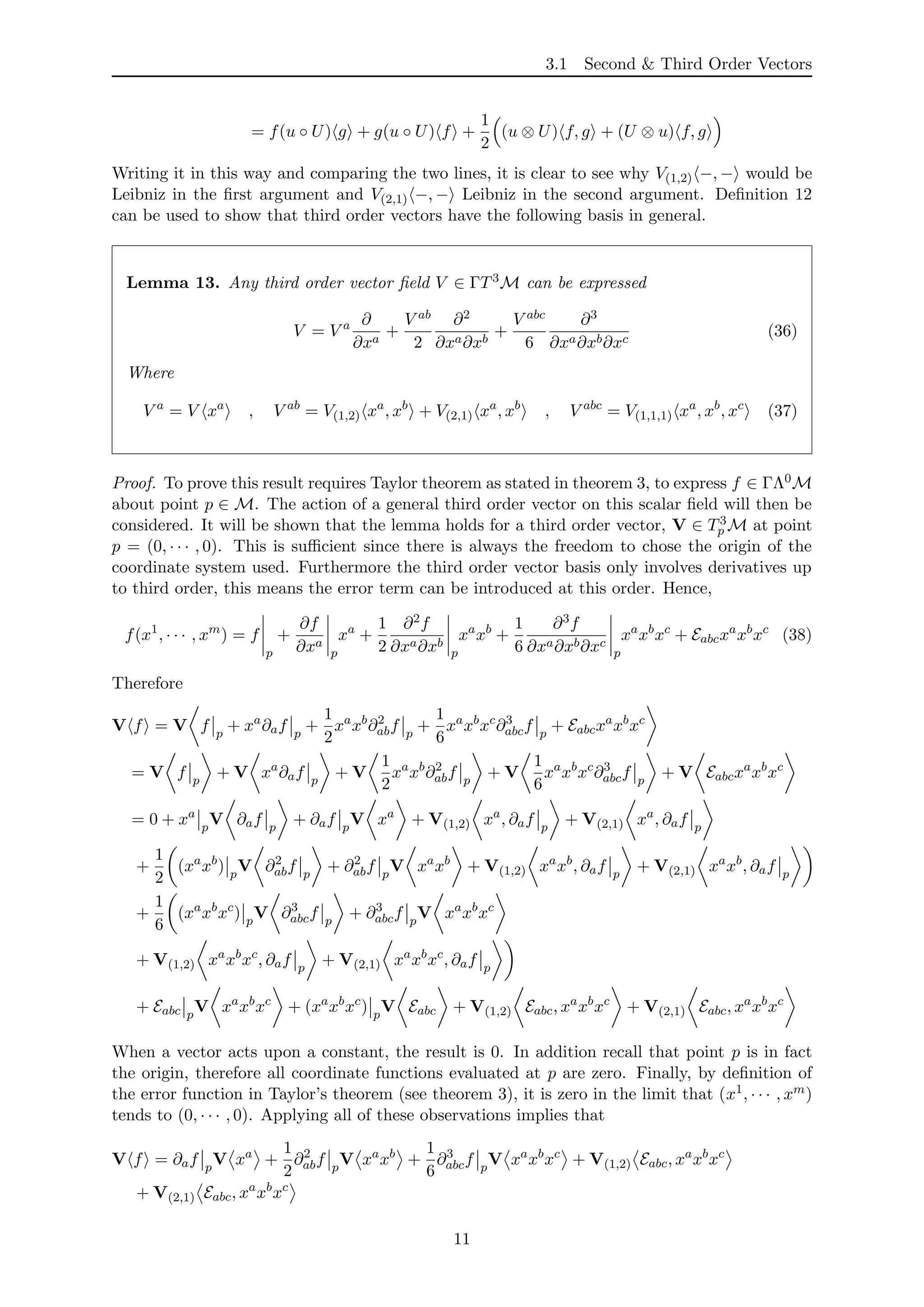
In section 3, the most general basis of a third order vector is stated and proved. Central to this
proof is the following version of Taylor’s theorem[9].
5](https://image.slidesharecdn.com/46491f5f-30bc-4c7a-99ba-d9cbbd913c19-150725210144-lva1-app6891/75/SubmissionCopyAlexanderBooth-5-2048.jpg)
![2.2 First Order Vectors & 1-Forms
Theorem 3. Given any function f ∈ ΓΛ0M that is differentiable at least q-times and described
by coordinates (x1, · · · , xm), it can be expressed about the point p = (0, · · · , 0) as
f(x1
, · · · , xm
) =
|I|≤q
DIf
I! p
xI
+
|I|=q
EI(x1
, · · · , xm
)xI
(3)
Where E(x1, · · · , xm) is a finite error term with the property that it is continuous and
lim
xa→0
EI(x1
, · · · , xm
) = 0 (4)
A full explanation of multi-index notation can be found in the glossary of notation, section 8.
Equipped with this formal treatment of coordinate systems, vector fields are considered next.
2.2 First Order Vectors & 1-Forms
Before talking about higher order vectors, it is useful to introduce the coordinate free definition
of a ‘regular’ vector. Regular vectors refer to the type of vector usually dealt with in classic
physics, such as those in mechanics. That is to say, in index notation they are defined as all
objects u = ua ∂
∂xa , whose components ua obey the following transformation law[12].
ˆuα
=
∂yα
∂xa
ua
(5)
For the remainder of the document, these vectors will be known as first order vectors. The
claim that all first order vectors can be written in the form u = ua ∂
∂xa will be covered by a more
general theorem in section 3.
In the language of differential geometry, a vector field v is defined as a function which takes a
scalar field f and gives v f , a new scalar field[11]. Here angular brackets are used for clarity,
avoiding any confusion between this type of action and simply listing a function and its variables.
For example, g(x, y) is a scalar field in x and y. In order for this to be a full and completely
equivalent definition of a vector field, the function must satisfy two properties[11].
Definition 4. Given f, g ∈ ΓΛ0M, a vector field v ∈ ΓTM is a function v : ΓΛ0M → ΓΛ0M,
with v : f → v f such that it satisfies
v f + g = v f + v g (6)
v fg = fv g + gv f (7)
Equation (6) ensures that a vector acting upon a sum of scalar fields, gives a sum of the vector
acting on each scalar. This is known as plus linearity. Equation (7) says that a vector acting
upon a product of scalars obeys the Leibniz rule.
Useful to keep in mind, yet far less important for the purposes of this project are 1-form fields.
They are defined in a similar way to vector fields but instead of following a Leibniz rule, they
are ‘f-linear’[11].
Definition 5. Given f ∈ ΓΛ0M and v, w ∈ ΓTM, a 1-form field µ ∈ ΓΛ1M is a function
µ : ΓTM → ΓΛ0M, with (v) → µ : v such that it satisfies
µ : (v + w) = µ : v + µ : w (8)
µ : (fv) = fµ : v (9)
6](https://image.slidesharecdn.com/46491f5f-30bc-4c7a-99ba-d9cbbd913c19-150725210144-lva1-app6891/75/SubmissionCopyAlexanderBooth-6-2048.jpg)
![2.3 The Connection
Intuitively if a particular operation is f-linear, it means that a scalar field can be ‘pulled out’ of
the operation. This is what is shown in equation (9). Exactly what is meant by f-linearity will
become clear as the report moves forward. An alternative definition of a tensor for example is
to view them as objects that are both plus and f-linear. Note the use of the colon, also seen
later in the project to represent a higher order vector combining with the connection.
In complete analogy with a first order vector field, given an m-dimensional manifold M with
coordinates (x1, · · · , xm), dxa for a = 1, · · · , m denotes a 1-form basis on this manifold[12]. It
is possible to construct differential forms of arbitrary degree, the process by which this is done
is explained in section A. These higher order differential forms are a far more well established
tool in mathematics and physics than higher order vectors.
2.3 The Connection
Of central importance to this project is the connection, appearing greatly in sections 5
onwards. As previously explained, when dealing with vectors it is sometimes called the covariant
derivative and represents differentiation of one vector field along another. This research only
considers the combination of the connection with first and higher order vectors, although its
action is defined on any tensor. Before considering the connection in a coordinate free way, it
is useful to look at it using index notation. To do this, the following objects must be defined.
Definition 6. Given a general connection on M,
Γc
ab = ∂a ∂b xc
(10)
Are the Christoffel Symbols of the second kind[11].
It can be shown that given a metric compatible and torsion free connection, the Christoffel
symbols are objects which can be written as a product of partial derivatives of the metric and
the inverse metric[11]. Metric compatibility describes the condition that the covariant derivative
of the metric is zero. In this project, the explicit form of these symbols is never required. With
definition 6 in mind and using classical tensor analysis, the covariant derivative of a vector
v ∈ ΓTM in the direction of a vector u ∈ ΓTM can be calculated.
( uv)c
= ua
∂a vb
∂b
c
= ua
∂a vb
c
∂b + ua
vb
∂a ∂b
c
(11)
The covariant derivative of vb, ∂a vb is just the partial derivative of vb with respect to xa and
using equation (10) it follows that
( uv)c
= ua ∂vc
∂xa
+ ua
vb
Γc
ab = u vc
+ ua
vb
Γc
ab (12)
As with a first order vector, defining the connection in a coordinate free way involves viewing
it as a function[11][12].
Definition 7. Given first order vector fields u, v, w ∈ ΓTM and f ∈ ΓΛ0M, a general con-
nection on M is a function : ΓTM × ΓTM → ΓTM, with (u, v) → uv such that it
satisfies
u (v + w) = uv + uw u (fv) = u f v + f uv (13)
(u+w)v = uv + wv (fu)v = f uv (14)
The equations in (13) ensure that the connection is plus linear and Leibniz in the vector being
differentiated. The equations in (14) on the other hand ensure that it is plus linear in the
direction being differentiated in, but instead of being Leibniz in this argument it is f-linear.
One further piece of notation featuring later in the text is 0, which is used to denote a torsion
free connection.
7](https://image.slidesharecdn.com/46491f5f-30bc-4c7a-99ba-d9cbbd913c19-150725210144-lva1-app6891/75/SubmissionCopyAlexanderBooth-7-2048.jpg)
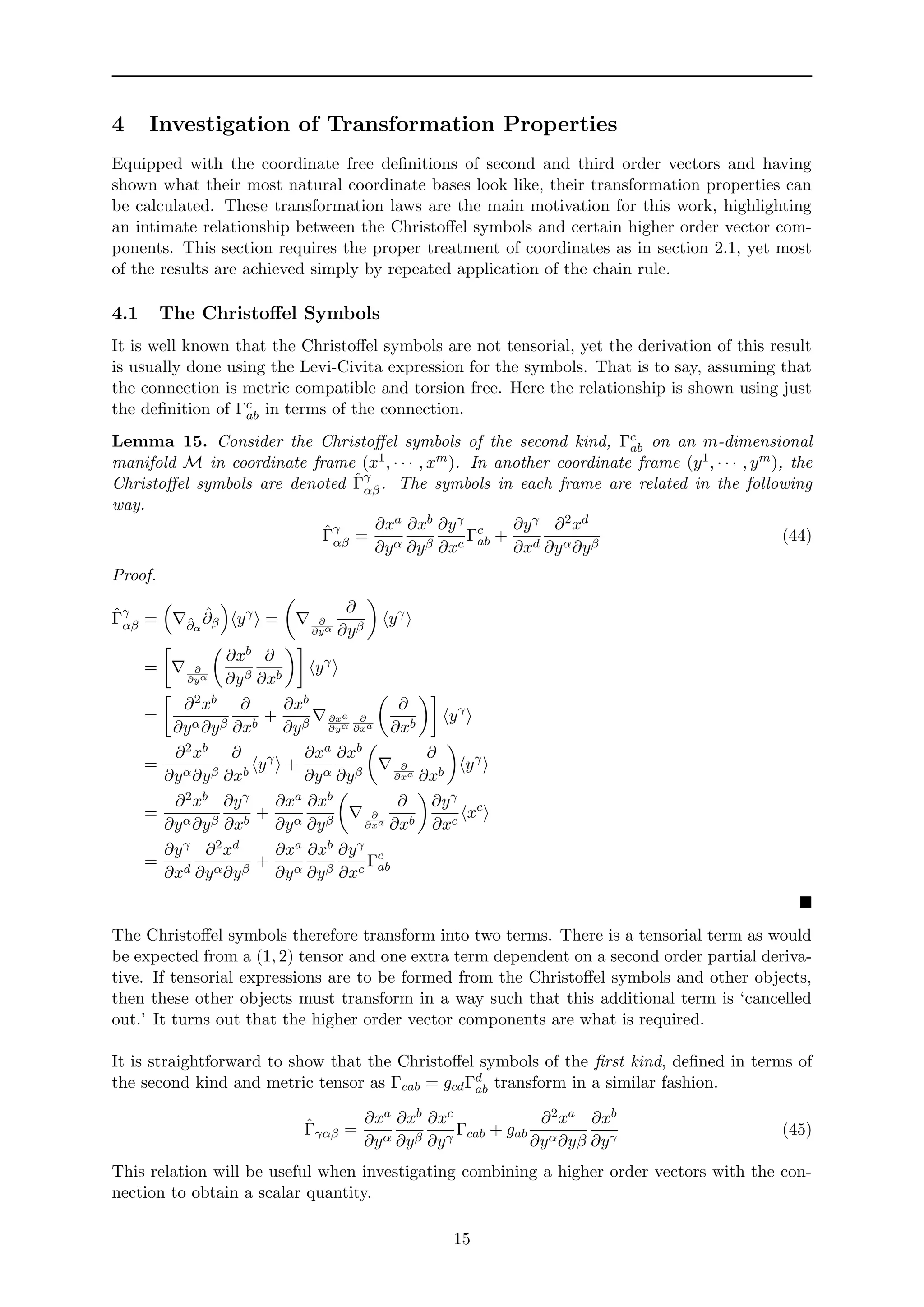
![2.4 Torsion & Curvature
2.4 Torsion & Curvature
Torsion and curvature are both tensorial quantities which appear in differential geometry, pro-
viding a way to quantify the warped nature of a particular manifold. Although Einstein’s
theory of gravity assumes a Levi-Civita connection, that is to say a connection which is metric
compatible and torsion free, curvature plays a central role. The Riemann curvature tensor fea-
tures explicitly not only in Einstein’s equation but also the geodesic deviation equation. This
relation quantifies the tidal forces between particles on neighbouring geodesics, a second or-
der effect[12]. It would be reasonable to assume therefore that somewhere in their definitions,
second derivatives and products of derivatives are involved.
Definition 8. Given first order vector fields u, v, w ∈ ΓTM, the curvature R of a connection
on M, is a function R : ΓTM × ΓTM × ΓTM → ΓTM, with (u, v, w) → R(u, v)w such
that
R(u, v)w = u vw − v uw − [u,v]w (15)
It is plus and f-linear in all of its arguments.
This object is sometimes known as the curvature vector[11]. The equivalent coordinate expres-
sion, viewing the curvature as a classical (1, 3) tensor is given by the following equation[12].
Re
bac = Γd
abΓe
cd + ∂aΓe
cb − Γd
cbΓe
ad − ∂cΓe
ab (16)
This report mostly deals with the coordinate free result.
Despite Einstein’s gravity only talking about the Levi-Civita connection, where possible in the
report, new objects are kept completely general. There are many alternative theories of gravity
such as Einstein-Cartan theory, which do involve torsion[4]. As such, the torsion tensor is now
defined[11][12].
Definition 9. Given first order vector fields u, v ∈ ΓTM, the torsion T of a connection on
M is a function T : ΓTM × ΓTM → ΓTM, with (u, v) → T (u, v) such that
T (u, v) = uv − vu − [u, v] (17)
It is plus and f-linear in all of its arguments.
As a classical tensor[12].
T c
ab = Γc
ab − Γc
ba (18)
Both the torsion and the curvature will be seen again in section 5, where an equation relating
the two will be required. An expression which does just this is Bianchi’s First Identity[8].
Ω R(u, v)w = Ω ( uT )(v, w) + T (T (u, v), w) (19)
Here Ω denotes the cyclic sum over u, v and w. Most notably when working in the torsion free
regime, this immediately reduces rather nicely to the following[12].
R(u, v)w + R(w, u)v + R(v, w)u = 0 (20)
All of the tools which form the foundation of the report’s proofs and definitions have now been
introduced. Next it is shown how higher order vectors are defined mathematically.
8](https://image.slidesharecdn.com/46491f5f-30bc-4c7a-99ba-d9cbbd913c19-150725210144-lva1-app6891/75/SubmissionCopyAlexanderBooth-8-2048.jpg)
![3 Introducing Higher Order Vectors
The main focus of this thesis is higher order vectors. There is a complete theory surrounding
differential forms of arbitrary order, yet work on arbitrary order vectors rarely features in the
literature. As has been mentioned, the notion of a higher order operator was introduced by
Duval in 1997 and their application to ordinary differential equations was recognised shortly
after[1][5]. All of what are believed to be new results established in this project, involve second
and third order vector fields. In the first part of this section therefore, particular attention is
paid to these. The second part of this section, section 3.2, introduces how higher order vectors
can be defined in general. Such a definition would be necessary if our research were to be
extended to arbitrary orders.
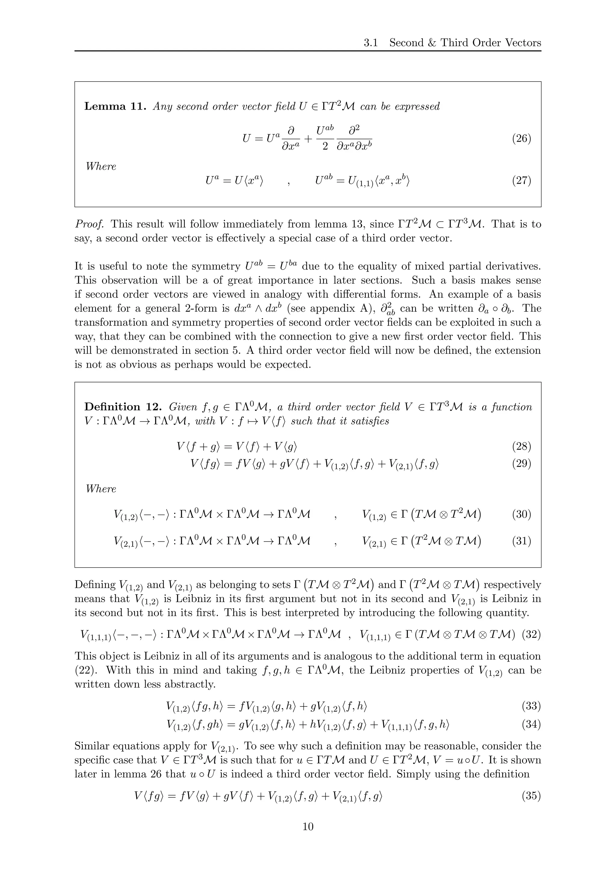
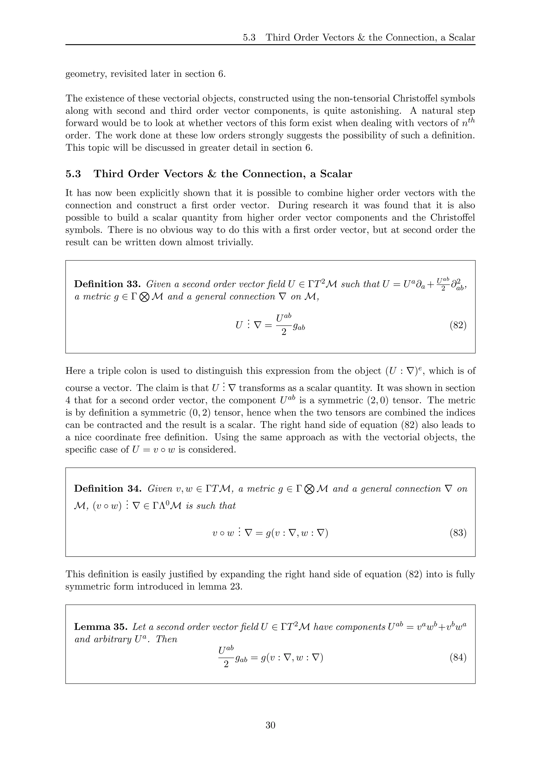
3.1 Second & Third Order Vectors
Beginning with the most simple extension to regular vector fields, second order vector fields.
The space of all second order vector fields is denoted ΓT2M. As with first order vectors, it
is possible to define them in a coordinate free way by means of a plus linearity condition and
Leibniz rule.
Definition 10. Given f, g ∈ ΓΛ0M, a second order vector field U ∈ ΓT2M is a function
U : ΓΛ0M → ΓΛ0M, with U : f → U f such that it satisfies
U f + g = U f + U g (21)
U fg = fU g + gU f + U(1,1) f, g (22)
Where
U(1,1) −, − : ΓΛ0
M × ΓΛ0
M → ΓΛ0
M , U(1,1) ∈ Γ (TM ⊗ TM) (23)
It is clear that this definition is similar to that of a first order vector field, equation (22) however
says that second order vector fields do not obey the standard Leibniz rule. When acting upon a
product of scalar fields there is the usual Leibniz part fU g +gU f as would be expected, but
then an extra term U(1,1) f, g . This object belongs to the set Γ (TM ⊗ TM) and is defined as
a function U(1,1) −, − : ΓΛ0M × ΓΛ0M → ΓΛ0M. These two properties mean that it is itself
Leibniz in both arguments. That is to say given h ∈ ΓΛ0M also
U(1,1) fg, h = fU(1,1) g, h + gU(1,1) f, h , U(1,1) f, gh = gU(1,1) f, h + hU(1,1) f, g (24)
Many will have written down a second order vector without realising. The Lie bracket of vectors
for example u, v , itself a vector, when written in a coordinate free way expands as
u, v f = u v f − v u f = u ◦ v f − v ◦ u f = (u ◦ v − v ◦ u) f (25)
Here the new notation u ◦ v is introduced, meaning ‘u operate v’. It is straightforward to
show that the object u ◦ v is a second order vector (see section 5.1). This simple example also
highlights the fact that it is possible to write a first order vector as a linear combination of
second order vectors. Not only does this rule extend to higher order vectors but implies that
ΓTM ⊂ ΓT2M. When looking for a general basis for this new space, it should include terms
similar to those bases of a first order vector. It will be proven at third order, but for now simply
stated in lemma 11, the most general form a second order vector field can take.
9](https://image.slidesharecdn.com/46491f5f-30bc-4c7a-99ba-d9cbbd913c19-150725210144-lva1-app6891/75/SubmissionCopyAlexanderBooth-9-2048.jpg)
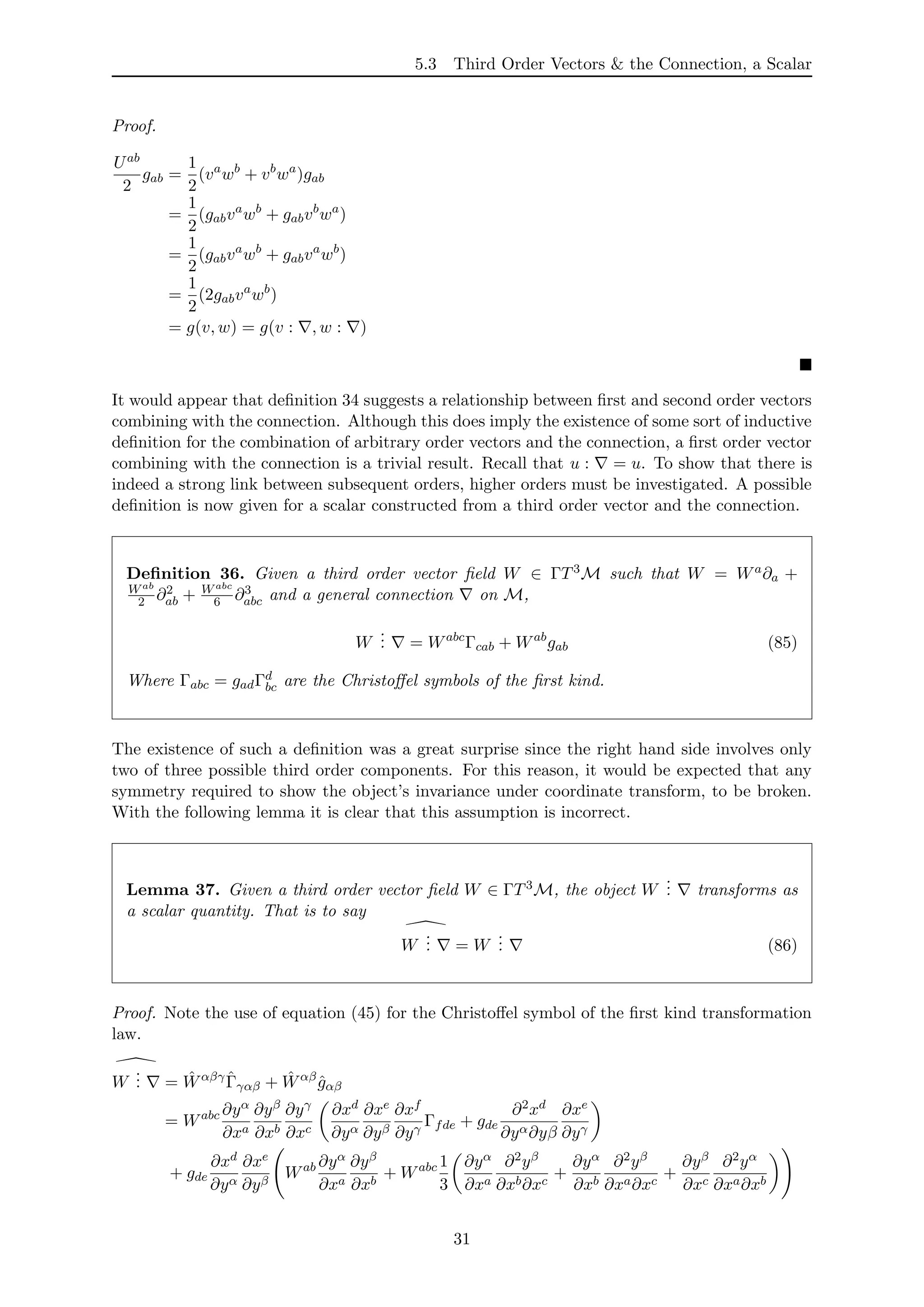
![3.3 Jet Spaces
Definition 14. Given f, g ∈ ΓΛ0M, an nth order vector field W ∈ ΓTnM is a function
W : ΓΛ0M → ΓΛ0M, with W : f → W f such that it satisfies
W f + g = W f + W g (40)
W fg = fW g + gW f +
a+b=n
W(a,b) f, g (41)
Where
W(a,b) −, − : ΓΛ0
M × ΓΛ0
M → ΓΛ0
M , W(a,b) ∈ Γ Ta
M ⊗ Tb
M (42)
In the case of a first order vector field n = 1, W(i,j) = 0 for all i and j since ΓT0M is not
explicitly defined. The summation runs over all possible combinations of a and b such that
a + b = n. It is clear to see that at large orders, things quickly become complicated. Take for
example W ∈ ΓT5M, equation (41) will include a term of the form W(3,2) ∈ Γ T3M ⊗ T2M .
In order to do any meaningful calculations, W(3,2) must be broken down into terms which are
Leibniz in most or all of their arguments, using a similar approach to that seen in the third
order case.
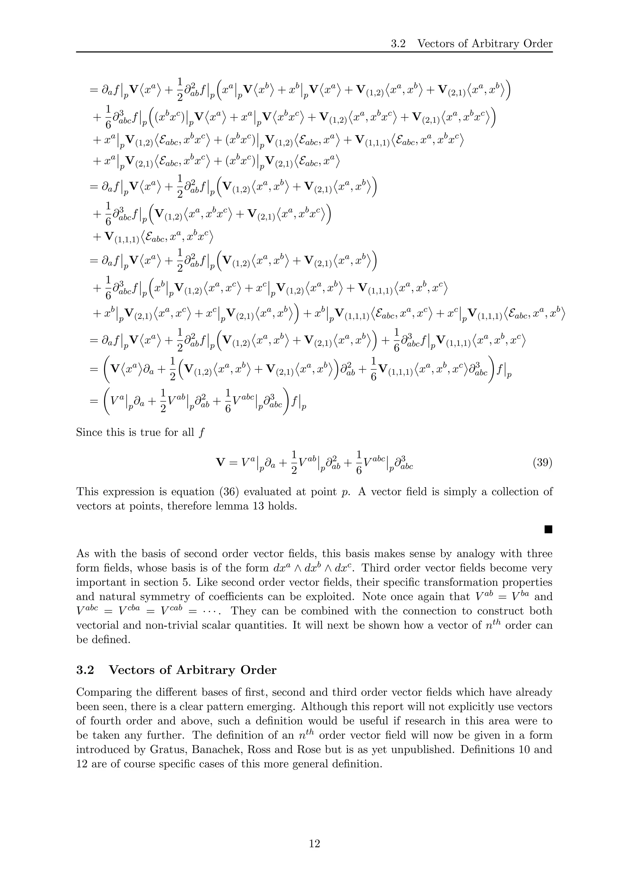
The most general basis of an nth order vector is as one would expect by extension of lemmas
11 and 13. The proof of the exact expression is however beyond the level of the report and is
largely irrelevant since our research involves vectors of order no higher than three.
3.3 Jet Spaces
It has been repeatedly highlighted that it is the specific transformation properties of higher order
vector components and the connection, which allows them to be combined in a meaningful way.
The foundation of this ‘natural relationship’ is in prolongation and jet spaces. Here a brief
overview of these ideas is presented. Consider first of all a scalar function f : M → R such that
f = f(x1, · · · , xm). The rth order jet space of f is denoted Jr(M → R) and is best understood
by considering the first few values of r. The zero jet of f, J0(M → R) is simply the set of all
functions {f : M → R} and is the bundle R × M over M[15]. It can be described therefore
by coordinates (x1, · · · , xm, f), meaning that the dimension of this jet space is m + 1. Higher
order jets can then be defined in a similar way, the table below shows the next three orders
of jets of f along with their corresponding coordinate system and dimension. The fractions
which appear in the expressions for the dimension of each space, are there to account for the
symmetries fab = fba, fabc = fbca = fcab = · · · and so on.
Jets of f. Bundle. Coordinate System. a, b, c ∈ [1, · · · , m] Dimension.
J0(M → R) R × M (xa, f) m + 1
J1(M → R) R × T∗M (xa, f, fa) 2m + 1
J2(M → R) - (xa, f, fa, fab) 1
2m2 + 2m + 1
J3(M → R) - (xa, f, fa, fab, fabc) 1
6m3 + 1
2m2 + 2m + 1
Table 1: Jets of f.
Here T∗M refers to the dual space of TM. Now take for example the third order jet of f, J3f
and consider the most general form of the third order vector V ∈ ΓT3M shown in equation
(36). Given an element of this jet space 3ϕ = (xa, ϕ, ϕa, ϕab, ϕabc) and the higher order vector
components V a, V ab and V abc, they can be combined in the following way.
V : 3
ϕ = V •
f(3
ϕ) + V a
fa(3
ϕ) +
1
2
V ab
fab(3
ϕ) +
1
6
V abc
fabc(3
ϕ) (43)
13](https://image.slidesharecdn.com/46491f5f-30bc-4c7a-99ba-d9cbbd913c19-150725210144-lva1-app6891/75/SubmissionCopyAlexanderBooth-13-2048.jpg)
![3.3 Jet Spaces
Where V • is known as the secular component and is included in some definitions of higher order
vectors. Duval’s work on differential operators for example does include this term[5]. In this
report however it was decided that the term be quotiented out of the higher order vector space.
This is equivalent to taking V • = 0. An element of the third order jet space is said to be the
third prolongation of f, if all of the Latin subscripts correspond to partial differentiation. That
is to say, fa(3ϕ) = ∂aϕ, fab(3ϕ) = ∂2
abϕ and so on. If it is assumed that in equation (43),
V • = 0 and it is the prolongation being dealt with then
V : 3
ϕ = V a ∂ϕ
∂xa
+
1
2
V ab ∂2ϕ
∂xa∂xb
+
1
6
V abc ∂3ϕ
∂xa∂xb∂xc
= V ϕ
That is to say, combining a third order vector with the third prolongation of f (secular term
quotiented out), corresponds to our definition of a higher order vector acting upon a scalar field.
The third order vector components therefore belong to the dual of jet J3f, denoted (J3f)∗.
It will later be shown in section 5 that taking combinations of higher order vector compo-
nents and the connection, leads to the cancellation of non-tensorial terms. This is because the
Christoffel symbols which ultimately define the connection, belong to the first order jet space
on M. That is to say given a connection on M, Γ : M → J1M where J1M is the set of all
first order jets on M[14].
14](https://image.slidesharecdn.com/46491f5f-30bc-4c7a-99ba-d9cbbd913c19-150725210144-lva1-app6891/75/SubmissionCopyAlexanderBooth-14-2048.jpg)
![5.1 Second Order Vectors & the Connection
= ( vw)c
+
1
2
vb
wa
T c
ab
∂
∂xc
= ( vw)c
−
1
2
vb
wa
T c
ba
∂
∂xc
= ( vw)c
−
1
2
T (v, w)c ∂
∂xc
= vw −
1
2
T (v, w)
To begin analysing this result, the choice of the second order vector components Ua and Uab
must be justified. As discussed in section 3.1, it is a straight forward exercise to prove that for
v, w ∈ ΓTM, v ◦ w is a second order vector. This simple result will now be shown.
Lemma 23. Given v, w ∈ ΓTM, then U ∈ ΓT2M if
U = v ◦ w (57)
Furthermore in index notation this may be written
U = va ∂wb
∂xa
∂
∂xb
+
vbwa + vawb
2
∂2
∂xa∂xb
(58)
Proof. This proof begins using definition 4 of a first order vector field.
U fg = (v ◦ w) fg = v w fg
= v fw g + gw f = v fw g + v gw f
= v f w g + fv w g + gv w f + v g w f
= fU g + gU f + v g w f + v f w g
= fU g + gU f + U(1,1) f, g
Where
U(1,1) f, g = v g w f + v f w g (59)
It is clear that U(1,1) f, g is Leibniz in both of its arguments, therefore v ◦ w ∈ ΓT2M by
definition 10. Next consider a similar calculation using indices and with f ∈ ΓΛ0M.
U f = (v ◦ w) f = v w f
= v wa ∂f
∂xa
= vb ∂
∂xb
wa ∂f
∂xa
= vb ∂wa
∂xb
∂f
∂xa
+ vb
wa ∂2f
∂xb∂xa
= vb ∂wa
∂xb
∂
∂xa
+ vb
wa ∂2
∂xb∂xa
f = vb ∂wa
∂xb
∂
∂xa
+
vbwa + vawb
2
∂2
∂xa∂xb
f
The final step exploits the natural symmetry in the definition of a second order vector, namely
Uab = Uba. This is true for all f therefore after relabelling, the final line is exactly equation
(58).
The notation (v◦w) : used in definition 21 is therefore perfectly logical. The choices of Ua and
Uab made in this definition correspond exactly to the calculated first and second components
of v ◦ w respectively.
There are two other observations which further justify the suitability of this definition. First of
all, it is clear to see that any first order vectors v, w ∈ ΓTM must satisfy by definition of the
Lie bracket
v ◦ w − w ◦ v − [v, w] = 0 (60)
Immediately then, the following is also true.
(v ◦ w − w ◦ v − [v, w]) : = (v ◦ w) : − (w ◦ v) : − [v, w] : = 0 (61)
Definition 21 must be consistent with this equation.
20](https://image.slidesharecdn.com/46491f5f-30bc-4c7a-99ba-d9cbbd913c19-150725210144-lva1-app6891/75/SubmissionCopyAlexanderBooth-20-2048.jpg)
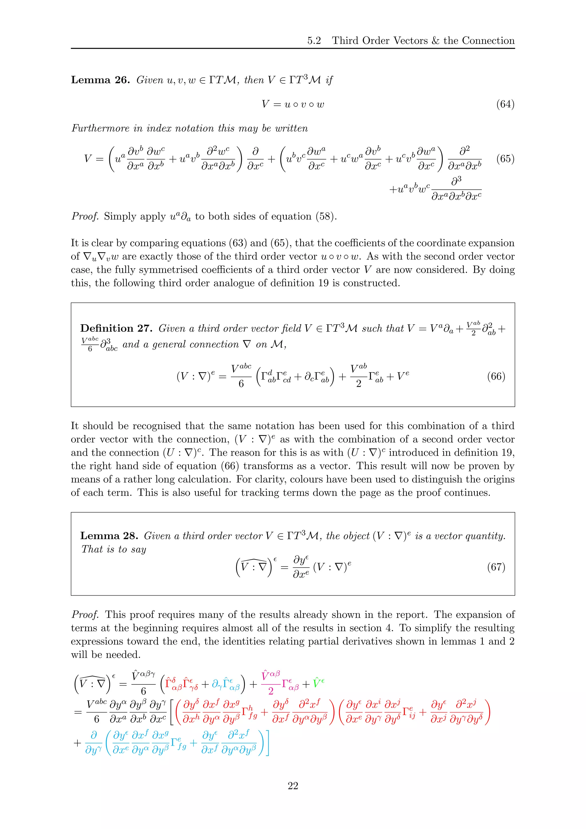
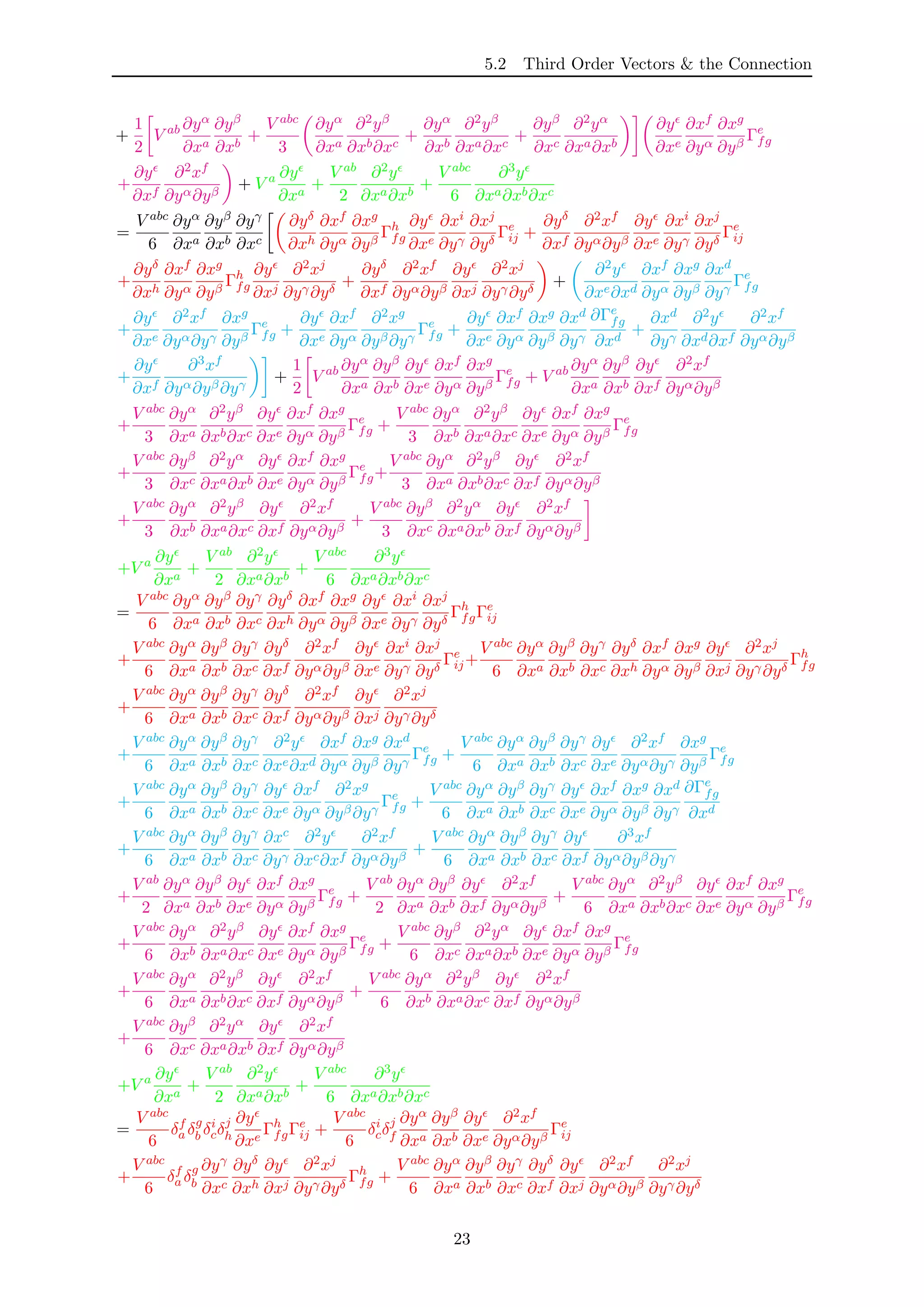
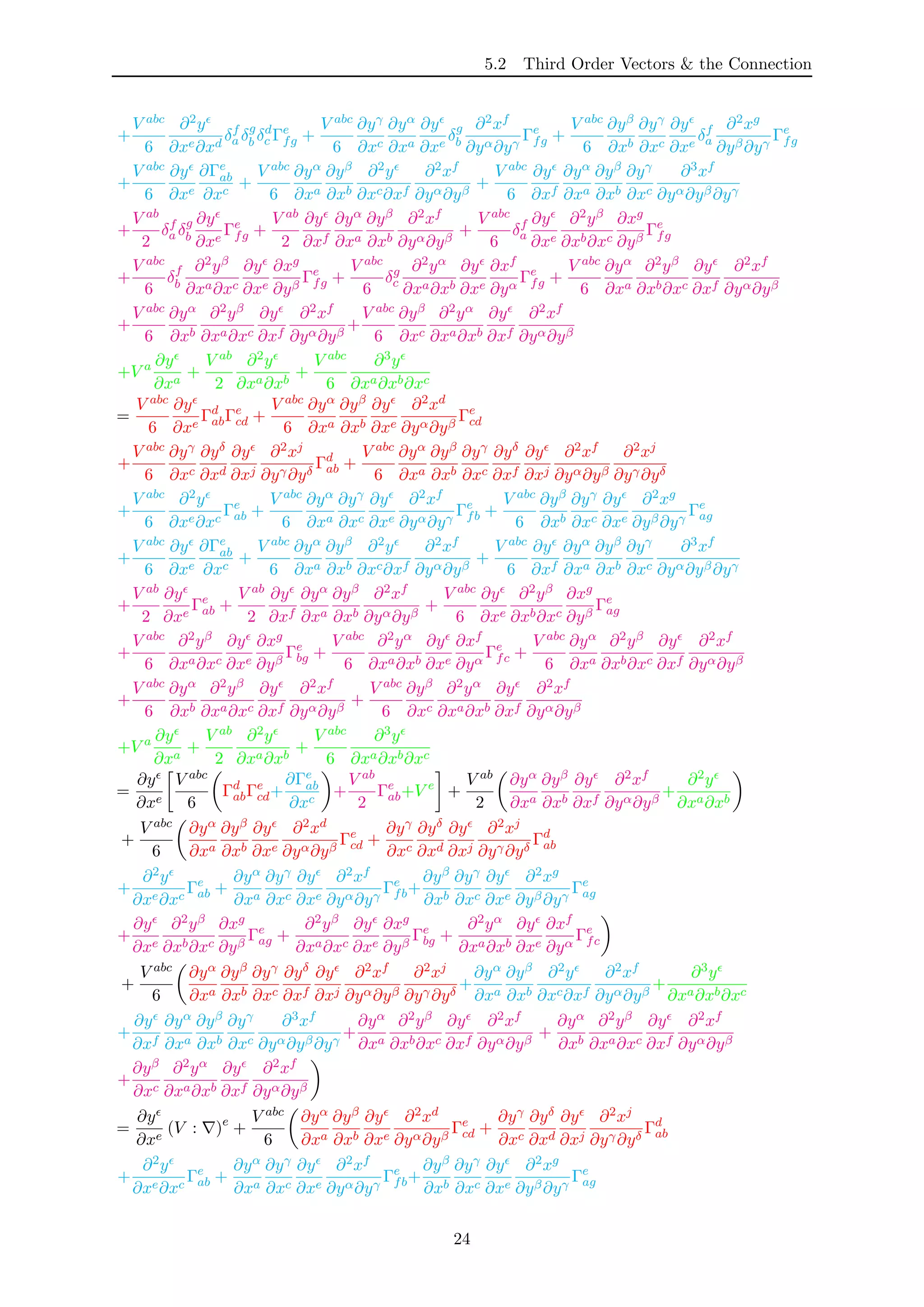
![5.2 Third Order Vectors & the Connection
Lemma 24. Given a general connection on M, (u ◦ v) : ∈ ΓTM satisfies
(v ◦ w) : − (w ◦ v) : − [v, w] : = 0 (62)
Proof. Since the Lie bracket of two vector fields is itself a vector field, definition 18 of a first
order vector field combining with the connection will be required.
(v ◦ w) : − (w ◦ v) : − [v, w] : = vw −
1
2
T (v, w) − wv −
1
2
T (w, v) − [v, w]
= ( vw − wv − [v, w]) −
1
2
T (v, w) +
1
2
T (w, v)
= T (v, w) − T (v, w)
= 0
The second observation is that the coordinate expression for (U : )e is very nearly the exact
component expansion of vw. It would therefore be expected that any additional terms in the
definition of (v◦w) : would involve first order covariant derivatives only. The torsion between
v and w, as stated in definition 9 is T (v, w) = vw − wv − [v, w], namely a sum of first order
covariant derivatives. Furthermore, the definition involves specifically two vectors, v and w.
A regular vector component must have only one free contravariant (upstairs) index. Simply
by considering the number of upstairs and downstairs indices in the coordinate expression, the
product vawb can only be multiplied by a tensor of the form Qc
ab. Torsion is the only candidate.
5.2 Third Order Vectors & the Connection
During initial research, the motivation for definition 19 originally came from considering the
coordinate expansion of vw. If the idea of combining a second order vector and the connection
is to be extended to third order, a natural consideration would be the coordinate expansion of
u vw.
Lemma 25. Given u, v, w ∈ ΓTM, then
( u vw)e
= uc
va
wb
Γe
abΓd
cd +
∂Γe
ab
∂xc
+ ua
vc
∂cwb
+ uc
wb
∂cva
+ uc
va
∂cwb
Γe
ab (63)
+uc
∂cvb
∂bwe
+ uc
vb
∂2
bcwe
Proof.
u( vw)e
= u va
wb
Γe
ab + va ∂we
∂xa
= uc
va
wb
Γf
ab + va ∂wf
∂xa
Γe
cf + uc ∂
∂xc
va
wb
Γe
ab + va ∂we
∂xa
= uc
va
wb
Γf
abΓe
cf + uc
va
Γe
cf
∂wf
∂xa
+ uc
va
wb ∂Γe
ab
∂xc
+ uc
va
Γe
ab
∂wb
∂xc
+ uc
wb
Γe
ab
∂va
∂xc
+ uc ∂va
∂xc
∂we
∂xa
+ uc
va ∂2we
∂xc∂xa
= uc
va
wb
Γf
abΓe
cf + uc
va
wb ∂Γe
ab
∂xc
+ Γe
ab ua
vc ∂wb
∂xc
+ uc
va ∂wb
∂xc
+ uc
wb ∂va
∂xc
+ uc ∂va
∂xc
∂we
∂xa
+ uc
va ∂2we
∂xc∂xa
At first sight this, equation (63) may not seem too enlightening. It is however straightforward
to show, using an identical method to that used to prove lemma 23, a similar lemma. Here it
is stated without proof.
21](https://image.slidesharecdn.com/46491f5f-30bc-4c7a-99ba-d9cbbd913c19-150725210144-lva1-app6891/75/SubmissionCopyAlexanderBooth-21-2048.jpg)
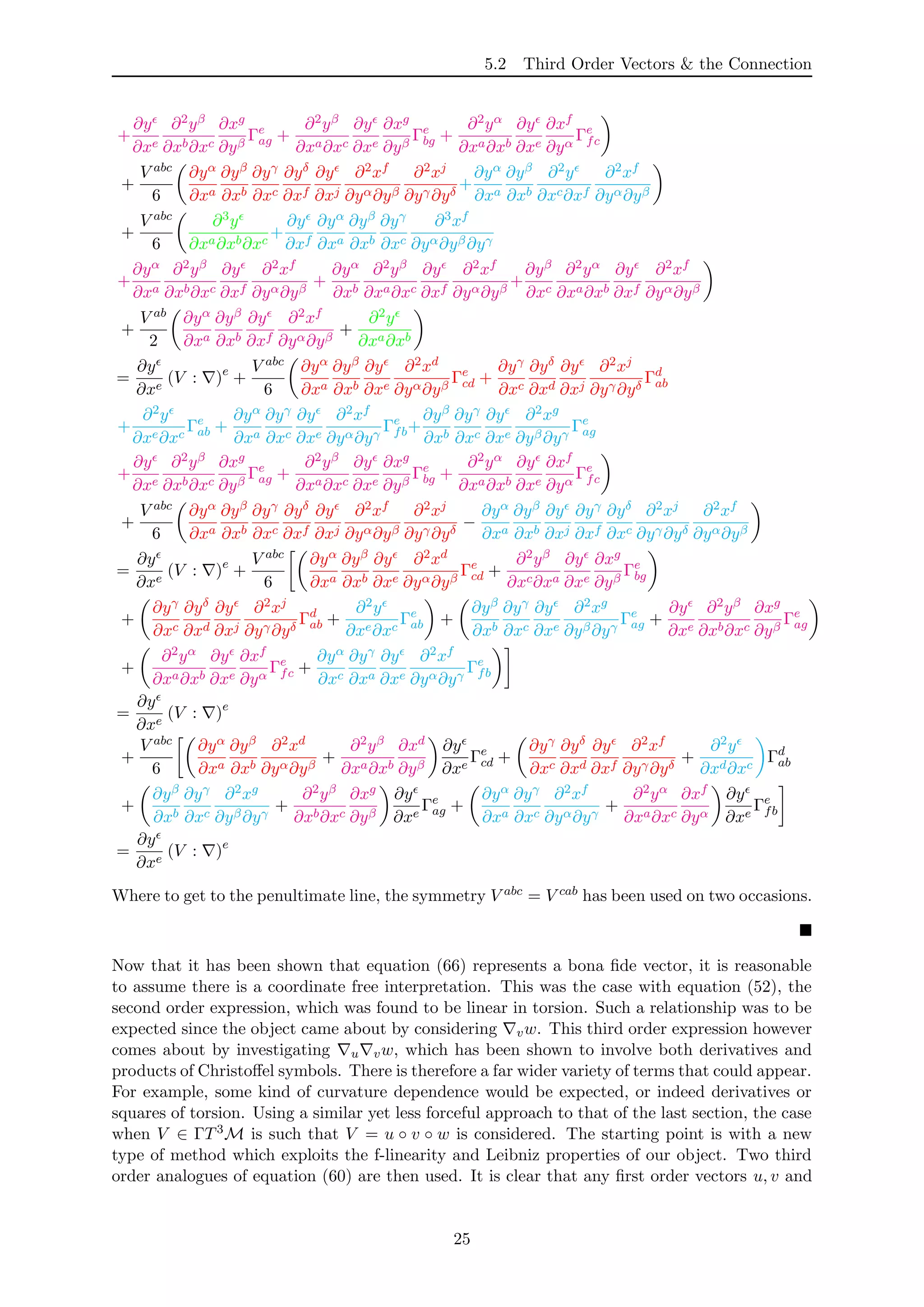
![5.2 Third Order Vectors & the Connection
w must satisfy both of the following identities.
u ◦ v ◦ w − v ◦ u ◦ w − [u, v] ◦ w = 0 (68)
u ◦ v ◦ w − u ◦ w ◦ v − u ◦ [v, w] = 0 (69)
In section 5.2.2, it is shown how these two equations alone can be used to justify a coordinate
free definition of (V : )e given a torsion free connection.
A Brief Aside
Looking back to section 5.1, the coordinate free definition of (v ◦w) : was ‘derived’ by writing
the coordinate expression in terms of vectors which have a specific coordinate free definition.
A significant amount of time was spent attempting to use the same method to get from the
coordinate to coordinate free definition of (V : )e. The main issue was finding the correct
interpretation for the third order vector component V abc. By definition of a higher order vector,
V abc is completely symmetric. That is to say, with the result of lemma 26, it would be expected
that V abc would take the following form for V = u ◦ v ◦ w.
V abc
∝ ua
vb
wc
+ ua
vc
wb
+ uc
va
wb
+ ub
va
wc
+ uc
vb
wa
+ ub
vc
wa
(70)
This way, V abc = V cba = V bca = · · · . On the other hand, in order to show that (V : )e
transforms as a vector (lemma 28), the only symmetry which is used is V abc = V cab. This is in
fact a cyclic permutation of abc and would imply that V abc could look something like
V abc
∝ A ua
vb
wc
+ uc
va
wb
+ ub
vc
wa
+ B ub
va
wc
+ ua
vc
wb
+ uc
vb
wa
(71)
For constants A and B. It is straightforward to show that this form of the component satisfies
V abc = V cab. Due to the length of each calculation that such a method involves, this turned out
to be a highly inefficient way of dealing with the problem and all attempts were unsuccessful.
For this reason a number of new, more indirect methods were developed. These were largely
more successful in directing the research toward a firm definition.
5.2.1 A General Connection
As has already been discussed, it is expected that a coordinate free (V : )e will involve
curvature terms and those which are derivatives of, or are second order in the torsion. One
other possibility are terms of the form T ( −−, −). These arise due to the appearance of
V ab ∝ ucwa∂cvb in the coordinate definition. To see how each of these terms feature, the
full coordinate free definition of (V : )e with a general connection will now be given. A
full justification will follow. As explained, due to lack of time and methods available, the
exact coefficients of each and every term were not calculated, however the overall form of the
expression is clear.
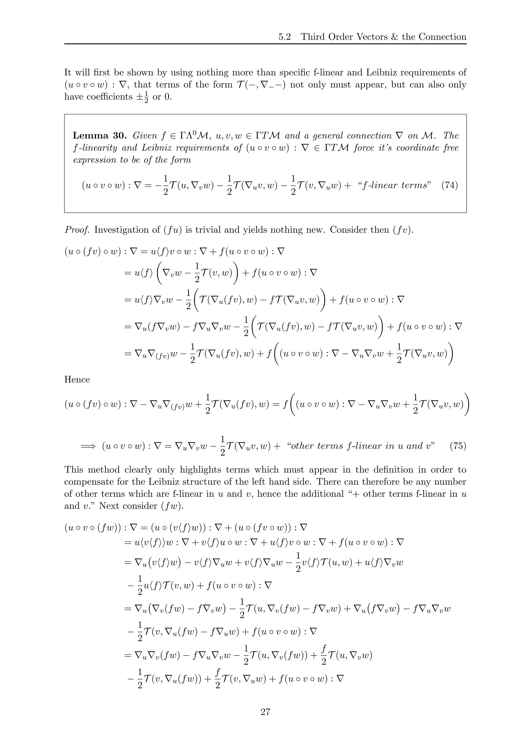
Definition 29. Given u, v, w ∈ ΓTM and a general connection on M,
(u ◦ v ◦ w) : ∈ ΓTM is such that
(u ◦ v ◦ w) : = u vw −
1
3
R(u, v)w −
1
3
R(u, w)v + ¯T3 (72)
Where
¯T3 = −
1
2
T (u, vw) −
1
2
T ( uv, w) −
1
2
T (v, uw) + A( uT )(v, w) + B( vT )(u, w) (73)
+C( wT )(u, v) + DT (T (u, v), w) + ET (T (v, u), w) + FT (T (w, u), v)
A, B, C, D, E and F are constants yet to be determined.
26](https://image.slidesharecdn.com/46491f5f-30bc-4c7a-99ba-d9cbbd913c19-150725210144-lva1-app6891/75/SubmissionCopyAlexanderBooth-26-2048.jpg)
![5.2 Third Order Vectors & the Connection
that the cyclic sum of three curvature tensors be zero. This means no more than two terms
of a cyclic sum can appear. Using Bianchi again, these two cyclic terms can be written as the
negative of the third term in the cyclic sum, hence no two terms which are cyclic permutations
of each other can appear simultaneously. Furthermore there are only two ways to arrange u, v
and w such that their cyclic sums are independent. That is to say, the cyclic sum of (u, w, v) is
only different to (u, v, w), not for example (w, v, u). This is easily verified by writing down all
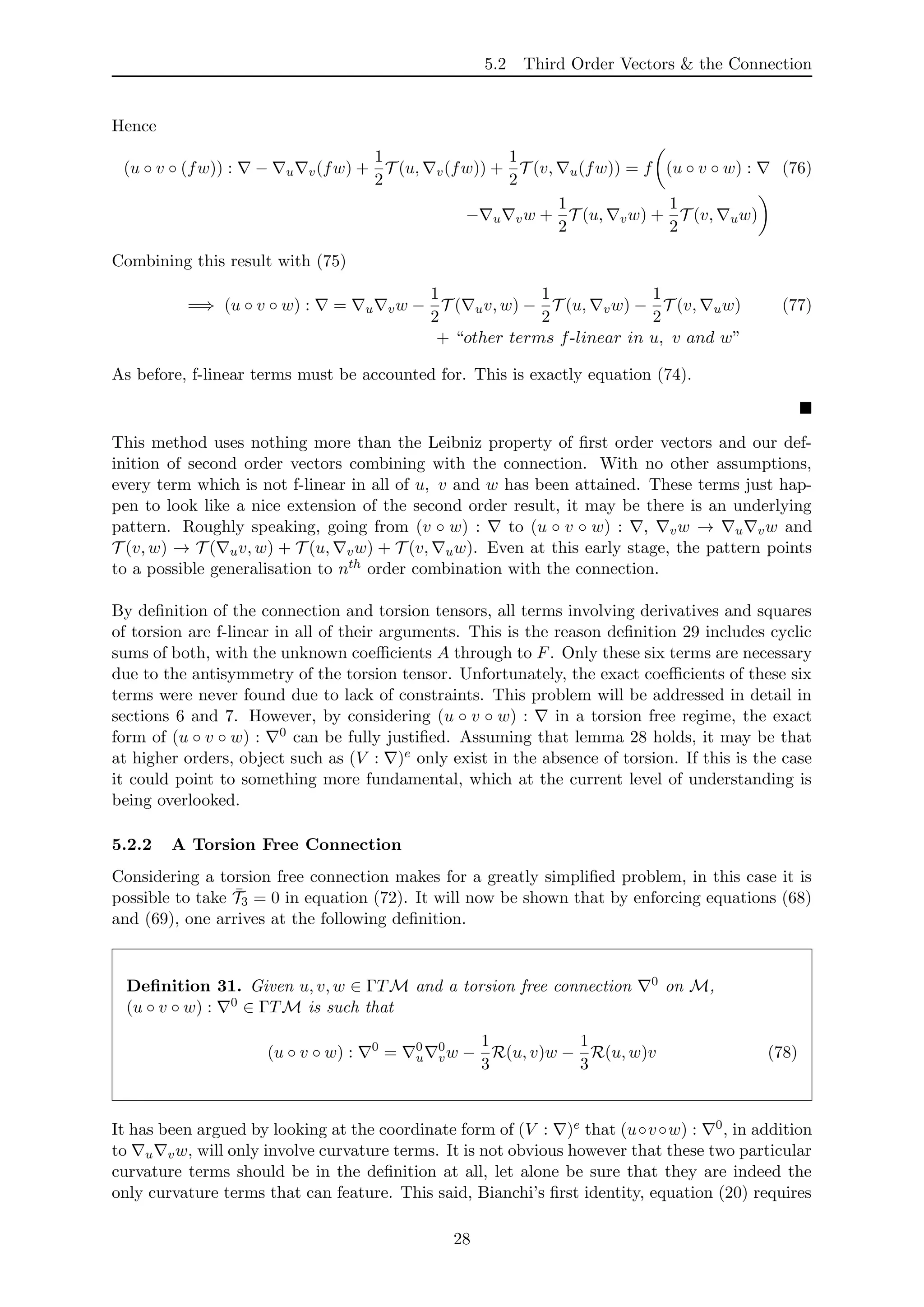
of the permutations. With these arguments alone, the following hypothesis can be made.
(u ◦ v ◦ w) : 0
= 0
u
0
vw + AR(u, v)w + BR(u, w)v (79)
Where A and B are constants. These constants can then be found using equations (68) and
(69). Instead of doing this calculation explicitly, it will simply be shown that (u ◦ v ◦ w) : 0
given by definition 31, does indeed satisfy both equations.
Lemma 32. Consider a torsion free connection 0 on M and (u ◦ v ◦ w) : 0 ∈ ΓTM such
that (u ◦ v ◦ w) : 0 = 0
u
0
vw − 1
3R(u, v)w − 1
3R(u, w)v. Then
u ◦ v ◦ w : 0
− v ◦ u ◦ w : 0
− [u, v] ◦ w : 0
= 0 (80)
u ◦ v ◦ w : 0
− u ◦ w ◦ v : 0
− u ◦ [v, w] : 0
= 0 (81)
Proof. Beginning with the left hand side of (80).
u ◦ v ◦ w : 0
− v ◦ u ◦ w : 0
− [u, v] ◦ w : 0
= 0
u
0
vw −
1
3
R(u, v)w −
1
3
R(u, w)v
− 0
v
0
uw −
1
3
R(v, u)w −
1
3
R(v, w)u − 0
[u,v]w
= 0
u
0
vw − 0
v
0
uw − 0
[u,v]w −
1
3
R(u, v)w −
1
3
R(u, w)v
+
1
3
R(v, u)w +
1
3
R(v, w)u
= R(u, v)w −
2
3
R(u, v)w +
1
3
R(v, w)u +
1
3
R(w, u)v
=
1
3
R(u, v)w + R(v, w)u + R(w, u)v = 0
By Bianchi’s first identity, equation (20). Now onto the left hand side of (81).
u ◦ v ◦ w : 0
− u ◦ w ◦ v : 0
− u ◦ [v, w] : 0
= 0
u
0
vw −
1
3
R(u, v)w −
1
3
R(u, w)v
− 0
u
0
wv −
1
3
R(u, w)v −
1
3
R(u, v)w − 0
u[v, w]
= 0
u
0
vw − 0
wv − [v, w] −
1
3
R(u, v)w −
1
3
R(u, w)v
+
1
3
R(u, v)w +
1
3
R(u, w)v
= 0
u (T (v, w)) = 0
Since the connection is torsion free.
It would seem therefore that definition 31 correctly reflects how a third order vector combines
with a torsion free connection. For many applications in physics, a torsion free connection is all
that is required for a solid theory. As has already been mentioned, general relativity is based on
the idea of a torsion free connection[12]. There is also the Fundamental Theorem of Riemannian
29](https://image.slidesharecdn.com/46491f5f-30bc-4c7a-99ba-d9cbbd913c19-150725210144-lva1-app6891/75/SubmissionCopyAlexanderBooth-29-2048.jpg)
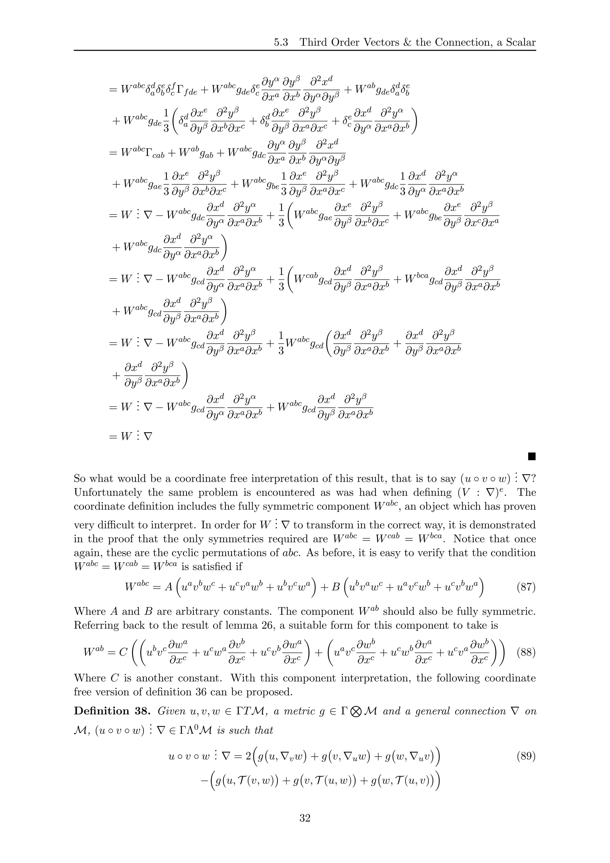
![5.3 Third Order Vectors & the Connection, a Scalar
This definition is justified by considering the coordinate expression of W
... and is the starting
point of the next lemma. The right hand side has been written in this way so that the torsion
and torsion free parts of W
... are clear. Later, this definition will be rewritten in a simpler
form.
Lemma 39. Take a metric g ∈ Γ M and let a third order vector field W ∈ ΓT3M have
components given by (87), (88) and arbitrary Wa. Then
Wabc
Γcab + Wab
gab = 2 g u, vw + g v, uw + g w, uv (90)
− g u, T (v, w) + g v, T (u, w) + g w, T (u, v)
Proof.
Wabc
Γcab + Wab
gab = A ua
vb
wc
+ uc
va
wb
+ ub
vc
wa
+ B ub
va
wc
+ ua
vc
wb
+ uc
vb
wa
Γcab
+ C ub
vc ∂wa
∂xc
+ uc
wa ∂vb
∂xc
+ uc
vb ∂wa
∂xc
+ ua
vc ∂wb
∂xc
+ uc
wb ∂va
∂xc
+ uc
va ∂wb
∂xc
gab
= gcd A Γd
abua
vb
wc
+ Γd
abuc
va
wb
+ Γd
abub
vc
wa
+ B Γd
abub
va
wc
+ Γd
abua
vc
wb
+ Γd
abuc
vb
wa
+ C ud
ve ∂wc
∂xe
+ ue
wc ∂vd
∂xe
+ ue
vd ∂wc
∂xe
+ uc
ve ∂wd
∂xe
+ ue
wd ∂vc
∂xe
+ ue
vc ∂wd
∂xe
= gcd A wc
( uv)d
− ue ∂vd
∂xe
+ uc
( vw)d
− ve ∂wd
∂xe
+ vc
( wu)d
− we ∂ud
∂xe
+ B wc
( vu)d
− ve ∂ud
∂xe
+ vc
( uw)d
− ue ∂wd
∂xe
+ uc
( wv)d
− we ∂vd
∂xe
+ C ud
ve ∂wc
∂xe
+ ue
wc ∂vd
∂xe
+ ue
vd ∂wc
∂xe
+ uc
ve ∂wd
∂xe
+ ue
wd ∂vc
∂xe
+ ue
vc ∂wd
∂xe
= Ag(w, uv) + Ag(u, vw) + Ag(v, wu) + Bg(w, vu) + Bg(v, uw) + Bg(u, wv)
+ gcd Cue
wc ∂vd
∂xe
− Awc
ue ∂vd
∂xe
+ Cuc
ve ∂wd
∂xe
− Auc
ve ∂wd
∂xe
+ Cue
vc ∂wd
∂xe
− Bue
vc ∂wd
∂xe
+ Cud
ve ∂wc
∂xe
− Bud
we ∂vc
∂xe
+ Cvd
ue ∂wc
∂xe
− Avd
we ∂uc
∂xe
+ Cwd
ue ∂vc
∂xe
− Bwd
ve ∂uc
∂xe
Taking A = B = C = 1.
= g(w, uv) + g(u, vw) + g(v, wu) + g(w, vu) + g(v, uw) + g(u, wv)
+ gcd ud
ve ∂wc
∂xe
− we ∂vc
∂xe
+ vd
ue ∂wc
∂xe
− we ∂uc
∂xe
+ wd
ue ∂vc
∂xe
− ve ∂uc
∂xe
= g(w, uv) + g(u, vw) + g(v, wu) + g(w, vu) + g(v, uw) + g(u, wv)
+ g([v, w], u) + g([u, w], v) + g([u, v], w)
= g(u, vw + wv + [v, w]) + g(v, wu + uw + [u, w]) + g(w, uv + vu + [u, v])
= g u, 2 vw − T (v, w) + g v, 2 uw − T (u, w) + g w, 2 uv − T (u, v)
= 2 g u, vw + g v, uw + g w, uv − g u, T (v, w) + g v, T (u, w) + g w, T (u, v)
33](https://image.slidesharecdn.com/46491f5f-30bc-4c7a-99ba-d9cbbd913c19-150725210144-lva1-app6891/75/SubmissionCopyAlexanderBooth-33-2048.jpg)
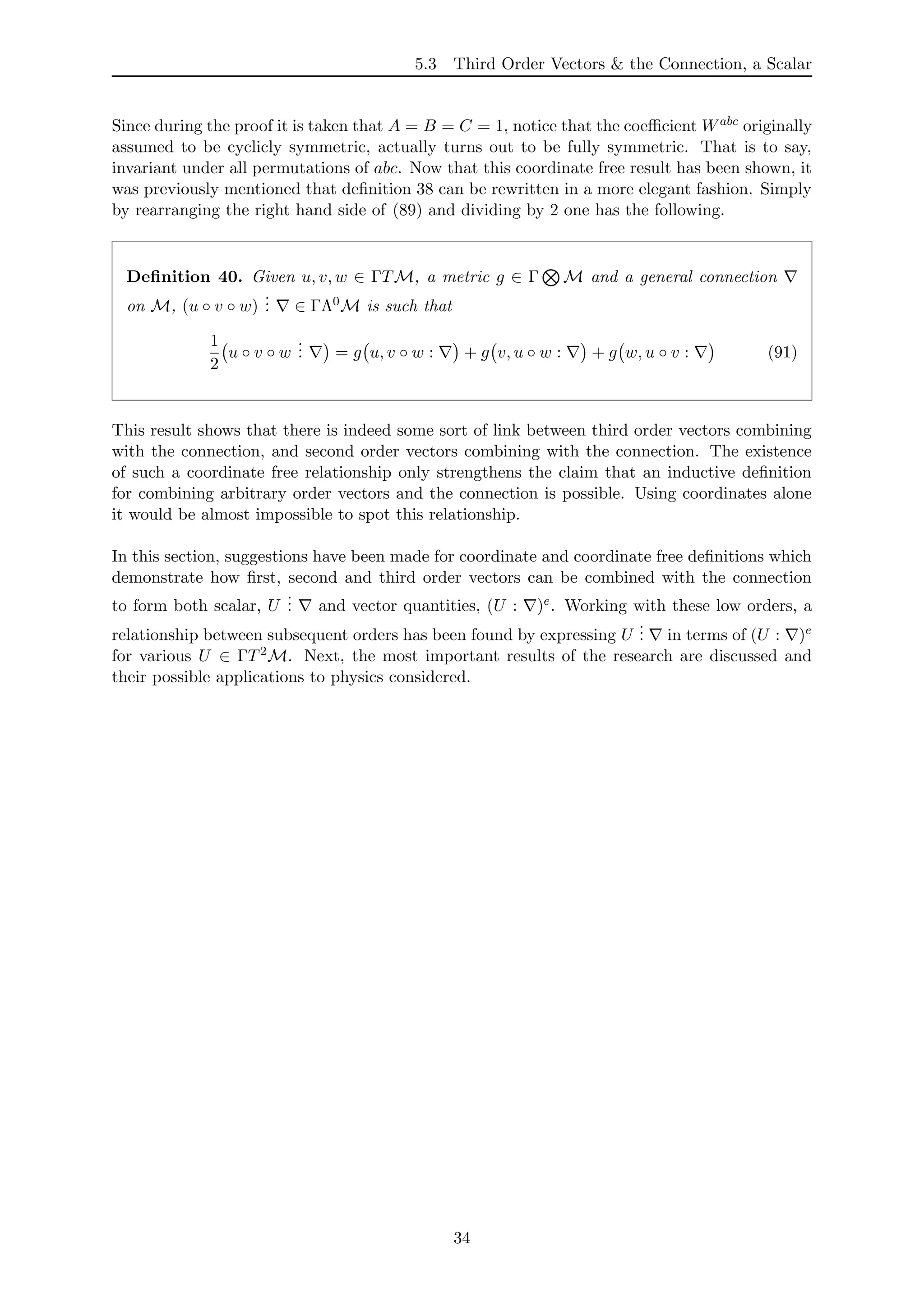
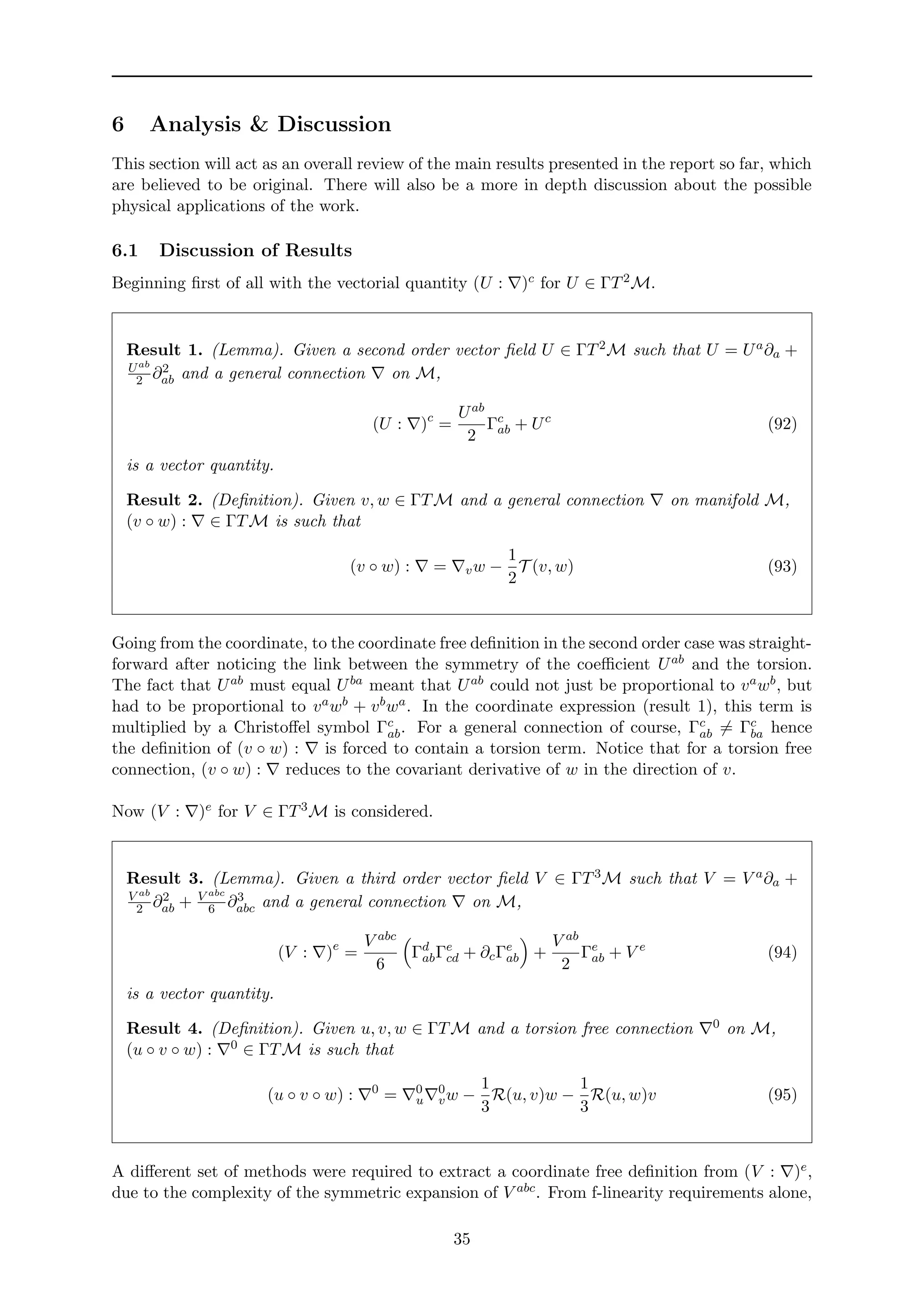
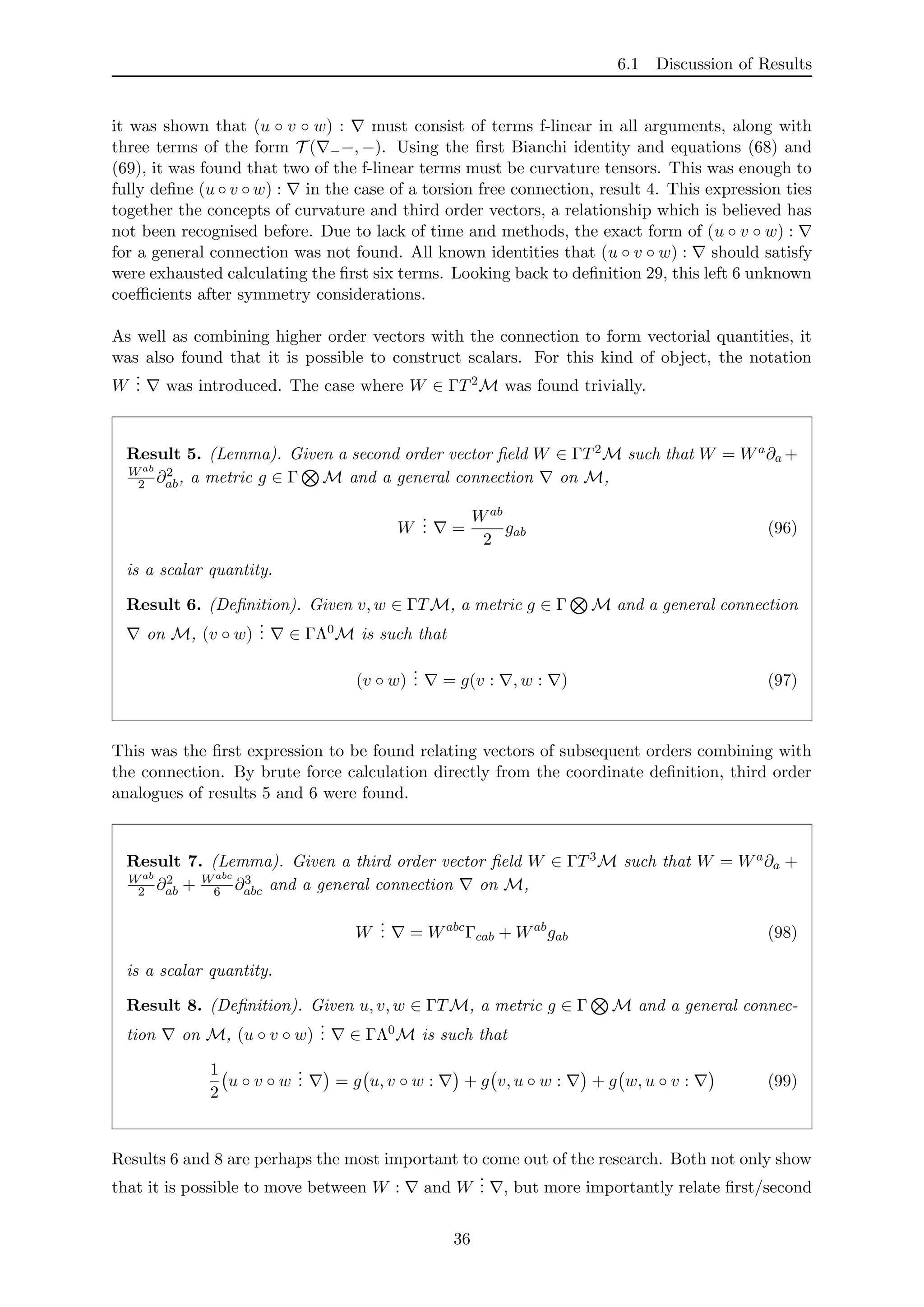
![6.2 Physical Applications
order vectors combining with the connection and second/third order vectors combining with
the connection respectively. As has already been highlighted, this points to a possible inductive
definition which combines arbitrary order vectors and the connection.
All eight of these results have arisen from a natural relationship between the connection and
the higher order vector components. It has been shown that both the Christoffel symbols
and higher order vector components are in general non-tensorial. Take the specific example of
U ∈ ΓT2M with first component, Ua. Under a change of coordinate frame, both transform
with a piece which is tensorial and an additional non-linear piece, dependant on second order
derivatives of each coordinate function. Combining the two together in the right way has the
effect of cancelling out the additional, non-tensorial term. It was explained in section 3.3 that
the fundamental reason for this cancellation is their dual jet space relationship.
6.2 Physical Applications
The study of higher order vectors is fairly abstract, yet it has been shown that combining them
with the connection leads to relationships between them and useful, measurable geometric
quantities. Covariant derivatives, curvature and torsion lend themselves well to the study of
gravity, where the nature of the space in question has direct consequence in the theory. General
relativity for example has the geodesic deviation equation. This equation states that the only
way gravity can be ‘measured’ is to look at the curvature of the manifold in which a test particle
moves[12]. It is natural then to expect, that it may be possible to express some equations from
Einstein’s theory, in terms of these new coordinate free objects. In lemma 41, the condition
which a vector must satisfy in order for it to be Killing is rewritten. A vector u ∈ ΓTM is
Killing if Lug = 0, that is to say that the Lie derivative of the metric in the direction of u is
zero[12]. Every Killing vector corresponds to a conserved quantity in the spacetime described
by g, energy or momentum for example[12]. It is straightforward to show assuming metric
compatibility and using the Leibniz rule that
Lug = 0 =⇒ u g(v, w) = g [u, v], w + g v, [u, w] (100)
For all v and w.
Lemma 41. Consider first order vectors u, v, w ∈ ΓTM, a metric g ∈ Γ M and a metric
compatible connection on M. u is a Killing vector if
u g(v, w) =
1
2
[u, v] ◦ w
... +
1
2
[u, w] ◦ v
... (101)
Proof. Beginning with equation (100). u is a Killing vector if for all v and w it satisfies
u g(v, w) = g [u, v], w + g v, [u, w] (102)
Now consider the following.
1
2
u ◦ v ◦ w
... −
1
2
v ◦ u ◦ w
... = g u, v ◦ w : + g v, u ◦ w : + g w, u ◦ v :
− g v, u ◦ w : − g u, v ◦ w : − g w, v ◦ u :
= g w, u ◦ v : − g w, v ◦ u :
= g w, [u, v] : = g w, [u, v]
37](https://image.slidesharecdn.com/46491f5f-30bc-4c7a-99ba-d9cbbd913c19-150725210144-lva1-app6891/75/SubmissionCopyAlexanderBooth-37-2048.jpg)
![6.2 Physical Applications
Then immediately by relabelling.
1
2
u ◦ w ◦ v
... −
1
2
w ◦ u ◦ v
... = g v, [u, w]
Substituting these two expressions directly into equation (102) gives
u g(v, w) =
1
2
u ◦ v ◦ w
... −
1
2
v ◦ u ◦ w
... +
1
2
u ◦ w ◦ v
... −
1
2
w ◦ u ◦ v
...
=
1
2
u ◦ v ◦ w − v ◦ u ◦ w
... +
1
2
u ◦ w ◦ v − w ◦ u ◦ v
...
=
1
2
[u, v] ◦ w
... +
1
2
[u, w] ◦ v
...
This is a nice result which involves both of the new second and third order scalar objects.
A possible application of the vectorial objects (U : )c in a similar area of physics, are to new
cosmological models. The method for doing such modelling usually begins with the construction
of a Lagrangian, which is then integrated to obtain the action. The equations which define the
physical laws of the universe in question, are obtained by finding the stationary points of the
action. In theory, the Lagrangian contains all of the necessary information for a complete
description of the physical system. For a given universe, it is sensible to require that the
Lagrangian be invariant under Lorentz group transformations. This assures that any equations
of motion respect special relativity. The requirement is satisfied by the following Lagrangian
which yields Maxwell’s equations in a vacuum[16].
LMaxwell = −
1
2
dA ∧ dA + A ∧ J (103)
Where A is the electromagnetic potential 1-form and J is the 4-current 1-form. The advantage
of using coordinate free language to write down this Lagrangian is that Lorentz invariance is
automatically built in. With this in mind, the following cosmological Lagrangian featuring
U ∈ ΓT2M such that U = v ◦ w for v, w ∈ ΓTM, can be suggested.
LT2M = κ1d(U : ) ∧ d(U : ) + κ2(U : ) ∧ (U : ) (104)
The first term is dynamical and the second corresponds to the field mass, each have a coupling
of κ1 and κ2 respectively. This is in complete analogy with the Lagrangian for a massive scalar
field given in (118). In accordance with equation (103), wedging each of the two forms must
give an overall 4-form. This can be achieved by setting (U : ) to be a 1-form on M. The
manifold M is 4-dimensional, which means that (U : ) is in fact a 3-form on M. The degrees
therefore add correctly when the two forms are wedged together. It is straightforward to check
that having (U : ) as a 1-form ensures that the dynamical term is also an overall 4-form. A
more detailed discussion of exterior calculus can be found in appendix section A.
By writing down this Lagrangian, second order vectors are being viewed as possible new sources
of matter. Looking back to the coordinate free result, result 2, this could be seen as a fairly
reasonable suggestion. The expression is written in terms of curvature and torsion, both of
which are quantities which play a central role in general relativity and Einstein-Cartan theory
respectively. The Einstein-Cartan model of gravity is similar to general relativity but with non-
zero torsion. It is believed that torsion may feature in a theory of gravity in order to capture
38](https://image.slidesharecdn.com/46491f5f-30bc-4c7a-99ba-d9cbbd913c19-150725210144-lva1-app6891/75/SubmissionCopyAlexanderBooth-38-2048.jpg)
![the effects of matter with spin[4]. It was suggested in a 2010 paper by Poplawski that torsion
can not only remove the big bang singularity, but also explain cosmic inflation by relaxing the
torsion free condition in the Friedman equations[13]. It has been shown in this report that even
when combining just second order vectors with the connection, a linear torsion is introduced
naturally. It is possible that the universe described by equation (104) has no big bang singular-
ity, but preserves all of the observed properties of general relativity. It is not just gravitational
models which make use of torsion. Another example is in the modelling of crystal defects in the
continuum, more specifically dislocations and disclinations[3]. The properties of such a space
lend themselves well to a description through torsion[3].
By the same justification as was used to write down LT2M, a second Lagrangian involving a
third order vector V ∈ ΓT3M such that V = u ◦ v ◦ w for u, v, w ∈ ΓTM, can be suggested.
LT3M = κ1d(V : ) ∧ d(V : ) + κ2(V : ) ∧ (V : ) (105)
Due to the definition of a third order vector combining with a general connection being incom-
plete, this Lagrangian would correspond to a torsion free theory. The Fundamental Theorem
of Riemannian geometry states however that given a metric, there is a unique connection on it
which is metric compatible and torsion free[11]. There is no reason to believe therefore that a
Lagrangian of this form, would not predict anything new or of consequence.
7 Conclusion
It has been shown that it is possible to combine higher order vectors and the connection in
such a way, that the resulting objects are expressible in terms of useful geometric quantities.
These results were formed on the assumption that such objects must exist, given the natural
relationship between the connection and higher order vectors, which becomes evident when the
respective transformation laws are compared. The coordinate definitions of these new objects
were obtained by writing down expressions involving products of Christoffel symbols and higher
order vector components, while ensuring the correct number of free indices to indicate vector and
scalar quantities. Once these expression were explicitly proven to be tensorial, the coordinate
free definitions were obtained by considering the special cases of second and third order vectors,
v◦w ∈ ΓT2M and u◦v◦w ∈ ΓT3M. In all but one case, complete definitions were obtained for
general connections by simply respecting the symmetries of the higher order components. This
approach was unsuccessful for the third order vectorial object, where new methods to decipher
the exact form had to be found. With 2 equations involving the Lie bracket, f-linearity and
symmetry considerations, and the Bianchi identities, the problem was reduced from 13 to 6
unknowns. From this a complete torsion free definition could be extracted. As explained, it
may be that the elusiveness of a definition fully inclusive of torsion, despite the result of lemma
28, implies some deeper problem which is currently being overlooked. The final outcome is a
set of coordinate free definitions showing how second and third order vectors can be combined
with the connection to obtain 2 vector quantities and 2 scalar quantities.
The physical implications of these definitions were discussed at length in section 6.2, highlighting
possible applications to gravitational and cosmological theories. It is the natural occurrence of
torsion in the definitions, a frequently overlooked quantity, which could lead to new predictions
in these fields. In order to draw something physical from a Lagrangian however, it must first be
integrated and varied. To extract anything meaningful from equations (104) and (105) would
39](https://image.slidesharecdn.com/46491f5f-30bc-4c7a-99ba-d9cbbd913c19-150725210144-lva1-app6891/75/SubmissionCopyAlexanderBooth-39-2048.jpg)
![therefore require a method of computing the functional derivative of U : . Such mathematics
has not yet been developed. Finally, notice that a significant portion of the work features a
connection and no metric. Questions can therefore be asked about the possibility of building a
manifold abstractly, with a connection and no metric.
If this work were to be taken further, the ultimate goal would be an inductive definition which
describes how an nth order vector can be combined with the connection in a coordinate free
way. Results 6 and 8 which relate higher order vectors of subsequent order combining with the
connection, only support the existence of such a definition. Looking at the first, second and
third order vectorial combinations with the connection, there is a clear pattern emerging. An
nth order definition is likely to be of the following form.
(u1 ◦ · · · ◦ un) : = u1 · · · un−1 un + Sn (106)
Where u1, · · · , un ∈ ΓTM and Sn : [ΓTM]n → ΓTM. That is to say Sn is a function which
takes n first order vectors and gives a first order vector. It is also reasonable to assume that
Sn will be made up completely of curvature and torsion tensors, along with their higher order
covariant derivatives and products. Sn may contain for example
( u1 · · · u4 u5 T )( u6 · · · un−4 un−3 un−2, un−1 un) (107)
Indeed, any combination of torsions, curvatures and del operators which can accommodate n
first order vectors are a possibility. It is clear from the rate of increase in complexity of Sn, that
working with higher orders would require a computer program. For example, the next logical
step would be to investigate (u1 ◦ u2 ◦ u3 ◦ u4) : , S4 could contain any of the following.
−R(−, −)−
( − −T )(−, −)
T ( −−, −−)
R(T (−, −), −)−
R( −−, −)−
( −T )( −−, −)
T (T (−, −), T (−, −))
R(−, −)T (−, −)
R(−, −) −−
( −T )(T (−, −), −)
T (T (T (−, −), −), −)
T (R(−, −)−, −)
Before taking into account any symmetries in the arguments of the vectors, there are 4! ways
in which 4 first order vectors can be placed into each of the slots. That makes for a grand
total of 288 unknowns. Furthermore, even with the aid of a computer program, solving such an
expression for the exact definition would require 288 conditions. Recall that for the third order
case there were still 6 unknowns, with no known method to reduce this number any further. A
possible solution which, due to lack of time was never developed far enough to contribute, is
observing that a general connection can be written in the following form.
= + αQ , α ∈ R, Q ∈ Γ M (108)
This is a one parameter family of diffeomorphisms. If for example it is chosen that the connection
be completely torsion free, it is straightforward to show that taking α = 1/2 and Q = T
satisfies this choice.
= +
1
2
T (109)
The connection is still any general connection. Equation (108) could be used to substitute
for in the incomplete coordinate free definition of (u ◦ v ◦ w) : . By then carefully choosing
different values of α, it may be that the remaining 6 unknowns could be extracted.
This masters project has been successful in defining two ways in which first, second and third
order vectors can be combined with the connection to form tensorial quantities. It is fair to
say that if equipped with the correct techniques, there are many ways in which the research
could be taken forward and continued. However, what more can efficiently be achieved without
the development of appropriate computational methods or a completely different approach, is
limited.
40](https://image.slidesharecdn.com/46491f5f-30bc-4c7a-99ba-d9cbbd913c19-150725210144-lva1-app6891/75/SubmissionCopyAlexanderBooth-40-2048.jpg)
![8 Glossary of Notation
This section acts as a quick reference for all
notation used in this report, that is to say no
rigorous definitions are given.
Multi-Index Notation
Given I = [i1, · · · , iq], then unless otherwise
stated.
|I| = i1 + · · · + iq , ||I|| = len{I} (110)
I! = i1! · · · iq! , xI
= xi1
1 · · · x
iq
q (111)
The multi-index partial derivative.
DI
=
∂
∂xi1
1
· · ·
∂
∂x
iq
q
(112)
Basic Latin and Greek Script
This excludes all types of vector and other ten-
sor spaces.
Notation Explanation
M A manifold.
m Dimension of M.
p A point on M.
n Order of a vector.
k Degree of a form.
a, b, c, · · · α, β, γ, · · · Free/dummy indices.
q, r Natural numbers.
I, J Multi-indices.
i1, · · · , iq Indices contained in I.
κq Coupling constants.
Vectors and Vector/Tensor Spaces
1st Order Vector nth Order Vector Scalar k-Form
At a Point, p u, v, w ∈ TpM U, V, W ∈ Tn
p M f|p, g|p, h|p n/a
At all Points u, v, w ∈ TM U, V, W ∈ TnM n/a n/a
Field u, v, w ∈ ΓTM U, V, W ∈ ΓT2M f, g, h, λ ∈ ΓΛ0M µ, ν, η ∈ ΓΛkM
‘At all points’ refers to the following disjoint
union, the set of all vectors at all points.
TM =
p∈M
TpM (113)
The set Γ M denotes the space of all tensor
fields on M.
Other Spaces, Objects & Operations
Coordinate Coordinate Free Explanation
ua∂af u f An arbitrary vector acting upon a scalar.
Not required. µ : v A arbitrary 1-form acting upon a vector.
Γcab, Γc
ab Not required. 1st and 2nd kind Christoffel symbols.
Not required. / 0 A general/torsion free connection.
T c
ab / uavbT c
ab T / T (u, v) Torsion tensor.
Rd
abc / ubvcwaRd
abc R / R(u, v)w Curvature tensor.
gab g(u, v) The metric tensor.
Not required. Jrf/(Jrf)∗ rth order jet/dual of jet of scalar f.
Not required. rϕ Element of rth order jet of scalar f.
ua∂a(vb∂b) u ◦ v Vector u operating/acting on vector v.
(U : )e
U :
Higher order vector combining with the
connection to form a vector.
W
... W
...
Higher order vector combining with the
connection to form a scalar.
Not required. Lu The Lie derivative in direction of u.
Not required. ˜g The metric dual.
Not required. The Hodge star operator.
Not required. d The exterior derivative.
Not required. ∧ The wedge product.
Not required. A/J Electromagnetic potential/4-current 1-forms.
41](https://image.slidesharecdn.com/46491f5f-30bc-4c7a-99ba-d9cbbd913c19-150725210144-lva1-app6891/75/SubmissionCopyAlexanderBooth-41-2048.jpg)
![Appendices
A Exterior Calculus
In section 6.2, possible applications of the work are discussed. In one example, two Lagrangians
are written down and analysed using aspects of differential geometry which are not required
anywhere else during the main research phase. These are the exterior derivative ‘d’, the metric
dual ‘˜g,’ the wedge product ‘∧’ and the Hodge star operator ‘ ’. For the purposes of this report,
that is to say in order to understand the Lagrangian application, only a basic knowledge of
these ideas is necessary. If a formal definition is not essential, it has not been included.
The wedge product, ∧. This operation allows higher degree differential forms to be con-
structed from 1-forms (as introduced in section 2.2). To build a 4-form for example, the type
required for Lagrangians (104) and (105), two 1-forms are first wedged together to give a 2-
form. Next, two of these 2-forms can be wedged to give an overall 4-form. In general the wedge
product can be seen as the following function[11].
Definition 42. Given µ ∈ ΓΛkM and ν ∈ ΓΛqM, the wedge product is a function ∧ : ΓΛkM×
ΓΛqM → ΓΛk+qM, with (µ, ν) → µ∧ν such that it is associative and has graded commutativity.
µ ∧ ν = (−1)kq
ν ∧ µ (114)
It is also plus and f-linear in all of its arguments.
Higher degree differential forms are a far more well established tool in physics and mathematics
than higher order vectors. It has already been mentioned that it is possible to reduce Maxwell’s
equations down to just two expressions. To do this the electric and magnetic fields are combined
into a single ‘electromagnetic’ 2-form[12].
Equipped with the wedge product and keeping in mind the 1-form basis introduced in section
2.2, the coordinate expression for a general k-form can be written down[12].
Lemma 43. Given an m-dimensional manifold M with coordinates (x1, · · · , xm) and multi-
indexed scalar fields fI ∈ ΓΛ0M, a general k-form on M, µ ∈ ΓΛkM can be expressed
µ =
1
k!
fIdxI
, dxI
= dxi1
∧ · · · ∧ dxim
(115)
The factor of 1
k! is to account for the symmetry in the wedge product due to its graded com-
mutativity. This coordinate expression will be used when talking about the Hodge star.
Hodge star, . Although this operator is used in Lagrangians (104) and (105) which are
coordinate free, for the purposes of the project it is best to define the Hodge star using index
notation. A succinct coordinate free definition by induction does exist, however it requires the
concept of internal contraction which does not feature in the report. The action of the Hodge
star on a general k-form is calculated in the following way[2].
Lemma 44. Given an m-dimensional manifold M with metric g ∈ Γ M, multi-indexed
scalar fields fI ∈ ΓΛ0M and a general k-form µ ∈ ΓΛkM such that µ = 1
k!fIdxI,
µ =
det(g)
k!(m − k)
gi1j1
· · · gikjk
εj1···jkjk+1···jm fi1···ik
dxjk+1
∧ · · · ∧ dxjm
(116)
Where εj1···jkjk+1···jm is the Levi-Civita symbol.
42](https://image.slidesharecdn.com/46491f5f-30bc-4c7a-99ba-d9cbbd913c19-150725210144-lva1-app6891/75/SubmissionCopyAlexanderBooth-42-2048.jpg)
![The Hodge star is therefore a function : ΓΛkM → ΓΛm−kM, taking a k-form and producing
an (m−k)-form. Most notably its definition is dependant on the choice of metric and dimension
of the manifold. Taking the wedge product of a form with its own Hodge dual results in a form
of maximum degree in that particular space. This is the property which has been used in the
discussion section to construct the two Lagrangians.
Exterior derivative, d. The exterior derivative is an operator which allows the degree of a
form to be increased by 1. As with most coordinate free objects, d can be defined as a function
which obeys a set of rules. Here it is sufficient to understand how the exterior derivative of a
differential form can be calculated using a coordinate basis[6][12].
Lemma 45. Given an m-dimensional manifold M with coordinates (x1, · · · , xm), multi-indexed
scalar fields fI ∈ ΓΛ0M and a general k-form µ ∈ ΓΛkM such that µ = 1
k!fIdxI,
dµ =
1
k!
∂fI
∂xj
dxj
∧ dxI
(117)
The original k-form has become a (k + 1)-form. It is straightforward to show that d2 = 0 due
to the equality of mixed partial derivatives[6]. If classical vectors in R3 are viewed as 1-forms,
this property can be used to demonstrate the well known result × g = 0, where g is any
well behaved scalar field[6]. The exterior derivative is used in Lagrangians (104) and (105) to
construct a kinetic term. This is in complete analogy with how kinetic and mass terms are built
into Lagrangians in quantum field theory. The Lagrangian for a free scalar field ψ with mass λ
is given by[17]
L =
1
2
(∂a
ψ)(∂aψ) −
1
2
λ2
ψ2
(118)
Using the differential geometric approach, partial derivative ∂a has been replaced by exterior
derivative d.
Metric dual, ˜g. The metric dual provides a way to transition between differential 1-forms and
first order vectors and vice-versa. The dual of a 1-form field µ ∈ ΓΛ1M for example, is denoted
˜µ and is a vector field. Formally, it is best understood through its coordinate free definition[7].
Definition 46. Given µ ∈ ΓΛ1M and ν ∈ ΓΛ1M and metric g ∈ Γ M, the metric dual is
a function ˜g : ΓΛ1M × ΓΛ1M → ΓΛ0M, with (µ, ν) → ˜g(µ, ν) such that
˜g(µ, ν) = g(˜µ, ˜ν) (119)
Such an operation therefore makes it possible to apply the work done with vectors in the research
phase of the project, to a covariant Lagrangian formalism.
43](https://image.slidesharecdn.com/46491f5f-30bc-4c7a-99ba-d9cbbd913c19-150725210144-lva1-app6891/75/SubmissionCopyAlexanderBooth-43-2048.jpg)
![REFERENCES
References
[1] Aghasi, M; Dodson, C; Galanis, G. & Suri, A. (2006). Infinite-dimensional second order
ordinary differential equations via T2M. Nonlinear Analysis 67(10). 2829-2838.
[2] Barrett, T. & Grimes, D. (1995). Advanced Electromagnetism: Foundations, Theory and
Applications. Singapore: World Scientific Publishing Co. Pte. Ltd.
[3] Bennett, D; Das, C; Laperashvili, H. & Nielsen, H. (2013). The relation between the model
of a crystal with defects and Plebanski’s theory of gravity. International Journal of Modern
Physics A 28(13). pp.1350044.
[4] Cartan, E. (1922) Sur une g´en´eralisation de la notion de courbure de Riemann et les espaces
`a torsion. Comptes Rendue Acad. Sci. 174. 593-595.
[5] Duval, C. & Ovsienko, V. (1997). Space of Second-Order Linear Differential Operators as
a Module over the Lie Algebra of Vector Fields. Advances in Mathematics 132, 316-331.
[6] Flanders, H. (1963). Differential Geometry with Applications to the Physical Sciences. New
York: Dover Publishing.
[7] G¨ockeler, M. & Sch¨ucker, T. (1989). Differential Geometry, Gauge Theories and Gravity.
Cambridge: Cambridge University Press.
[8] Jensen, S. (2005). General Relativity with Torsion: Extending Wald’s Chapter on Curva-
ture. Chicago: University of Chicago.
[9] K¨onigsberger, K. (2004). Analysis 2. Berlin: Springer-Verlag.
[10] Landau, L. & Lifshitz, L. (1987). Fluid Mechanics, Volume 6 of Course of Theoretical
Physics. Oxford: Pergamon Press.
[11] Lee, Jeffrey. (1956). Manifolds & Differential Geometry. Providence: American Mathemat-
ical Society.
[12] Misner, C; Thorne, K. & Wheeler, J. (1973). Gravitation. San Fransisco: W. H. Freeman.
[13] Poplawski, N. (2010). Cosmology with Torsion: An Alternative to Cosmic Inflation. Physics
Letters B 694(3). 181-185.
[14] Sardanashvily, G. (1994). Five Lectures on the Jet Methods in Field Theory. Moscow:
Department of Physics Moscow State University. arXiv:hep-th/9411089v1.
[15] Sardanashvily, G. (2009). Fibre Bundles, Jet Manifolds and Lagrangian Theory. Lec-
tures For Theoreticians. Moscow: Department of Physics Moscow State University.
arXiv:0908.1886.
[16] Stern, A; Tong, Y; Desbrun, M. & Marsden, J. (2008). Variational Integrators for Maxwell’s
Equations with Sources. arXiv:0803.2070v1.
[17] Thomson, M. (2013). Modern Particle Physics. Cambridge: Cambridge University Press.
44](https://image.slidesharecdn.com/46491f5f-30bc-4c7a-99ba-d9cbbd913c19-150725210144-lva1-app6891/75/SubmissionCopyAlexanderBooth-44-2048.jpg)