This document provides an introduction to principal component analysis (PCA), a technique for dimensionality reduction. PCA transforms a dataset consisting of observations with multiple correlated variables into a new dataset of linearly uncorrelated variables called principal components. It does this by identifying the directions (principal components) along which the variance in the data is maximized. The document uses a dataset of car features to illustrate how PCA projects the data points onto lines representing principal components to reduce redundancy in the data representation.
I am Martin J. I am a Digital Signal Processing Assignment Expert at matlabassignmentexperts.com. I hold a Ph.D. in Matlab, Arizona University, USA. I have been helping students with their homework for the past 6 years. I solve assignments related to Digital Signal Processing.
Visit matlabassignmentexperts.com or email info@matlabassignmentexperts.com.
You can also call on +1 678 648 4277 for any assistance with Digital Signal Processing Assignments.
I am Bryan K. I am a Matlab Assignment Expert at matlabassignmentexperts.com. I hold a Ph.D. in Matlab, University of Florida, USA. I have been helping students with their homework for the past 7 years. I solve assignments related to Discrete Fourier Transform.
Visit matlabassignmentexperts.com or email info@matlabassignmentexperts.com.
You can also call on +1 678 648 4277 for any assistance with Discrete Fourier Transform Assignments.
I am Simon M. I am an Environmental Engineering Assignment Expert at matlabassignmentexperts.com. I hold a Ph.D. in Environmental Engineering, Glasgow University, UK. I have been helping students with their assignments for the past 8 years. I solve assignments related to Environmental Engineering.
Visit matlabassignmentexperts.com or email info@matlabassignmentexperts.com. You can also call on +1 678 648 4277 for any assistance with Environmental Engineering Assignments.
Using several mathematical examples from three different authors in texts from different courses this paper illustrates the easier way to avoid confusions and always get the correct results with the least effort was to use the proposed Excel Gamma function explained in detail for the proper use of the Q(z) and ercf(x) functions in most communication courses. The paper serves as a tutorial and introduction for such functions
I am Kennedy L. I am a Digital Signal Processing Assignment Expert at matlabassignmentexperts.com. I hold a Ph.D. in Matlab, Monash University, Australia. I have been helping students with their homework for the past 6 years. I solve assignments related to Digital Signal Processing.
Visit matlabassignmentexperts.com or email info@matlabassignmentexperts.com.
You can also call on +1 678 648 4277 for any assistance with Digital Signal Processing Assignments.
I am Nikita L. I am a Digital Signal Processing Assignment Expert at matlabassignmentexperts.com. I hold a Ph.D. in Matlab, University of Alberta, Canada. I have been helping students with their homework for the past 5 years. I solve assignments related to Digital Signal Processing.
Visit matlabassignmentexperts.com or email info@matlabassignmentexperts.com.
You can also call on +1 678 648 4277 for any assistance with Digital Signal Processing Assignments.
"FingerPrint Recognition Using Principle Component Analysis(PCA)”Er. Arpit Sharma
Fingerprint recognition is one of the oldest and most popular biometric technologies and it is used in criminal investigations, civilian, commercial applications, and so on. Fingerprint matching is the process used to determine whether the two sets of fingerprints details come from the same finger or not. This work focuses on feature extraction and minutiae matching stage. There are many matching techniques used for fingerprint recognition systems such as minutiae based matching, pattern based matching, Correlation based matching, and image based matching.
A new method based upon Principal Component Analysis (PCA) for fingerprint enhancement is proposed in this paper. PCA is a useful statistical technique that has found application in fields such as face recognition and image compression, and is a common technique for finding patterns in data of high dimension. In the proposed method image is first decomposed into directional images using decimation free Directional Filter bank DDFB. Then PCA is applied to these directional fingerprint images which gives the PCA filtered images. Which are basically directional images? Then these directional images are reconstructed into one image which is the enhanced one. Simulation results are included illustrating the capability of the proposed method.
I am Boris M. I am a Computer Science Assignment Help Expert at programminghomeworkhelp.com. I hold MSc. in Programming, McGill University, Canada. I have been helping students with their homework for the past 7 years. I solve assignments related to Computer Science.
Visit programminghomeworkhelp.com or email support@programminghomeworkhelp.com.You can also call on +1 678 648 4277 for any assistance with Computer Science assignments.
I am Danny G . I am an Electrical Engineering Assignment Expert at matlabassignmentexperts.com. I hold a Ph.D. Matlab, Schiller International University, USA. I have been helping students with their homework for the past 9 years. I solve assignments related to Electrical Engineering.
Visit matlabassignmentexperts.com or email info@matlabassignmentexperts.com.
You can also call on +1 678 648 4277 for any assistance with Electrical Engineering Assignments.
Numerical approach of riemann-liouville fractional derivative operatorIJECEIAES
This article introduces some new straightforward and yet powerful formulas in the form of series solutions together with their residual errors for approximating the Riemann-Liouville fractional derivative operator. These formulas are derived by utilizing some of forthright computations, and by utilizing the so-called weighted mean value theorem (WMVT). Undoubtedly, such formulas will be extremely useful in establishing new approaches for several solutions of both linear and nonlinear fractionalorder differential equations. This assertion is confirmed by addressing several linear and nonlinear problems that illustrate the effectiveness and the practicability of the gained findings.
I am Kefa J. I am a Computer Science Assignment Help Expert at programminghomeworkhelp.com. I hold an Ph.D. in Programming, Princeton University, USA Profession.. I have been helping students with their homework for the past 5 years. I solve assignments related to Computer Science.
Visit programminghomeworkhelp.com or email support@programminghomeworkhelp.com.
You can also call on +1 678 648 4277 for any assistance with Computer Science assignments.
A block diagram uses blocks and lines to show the related functions of parts of an electric circuit or system. Such a diagram shows the normal order of progression of the signal through a circuit.
A system is an assembly of parts (components) connected together to perform a stated function.
The system may be comprises of:
• A number of individual components connected together
• A number of smaller units called subsystem.
o Each subsystem itself consists of individual parts
I am Anastasia S. I am a Signal Processing Assignment Expert at matlabassignmentexperts.com. I hold a Masters's in Matlab from, Clemson University, USA. I have been helping students with their assignments for the past 6 years. I solve assignments related to Signal Processing.
Visit matlabassignmentexperts.com or email info@matlabassignmentexperts.com. You can also call on +1 678 648 4277 for any assistance with Signal Processing Assignments.
CEE 213—Deformable Solids The Mechanics Project Arizona Stat.docxcravennichole326
CEE 213—Deformable Solids The Mechanics Project
Arizona State University CP 1—Axial Bar
Computing Project 1
Axial Bar
The computing project Axial Bar concerns the solution of the problem of a prismatic bar
in a uniaxial state of stress with a variable load. The goal is to write a MATLAB program
that will allow the solution for a variety of load distributions and for all possible bounda-
ry conditions (i.e., fixed or free at either end).
The theory needed to execute this project is contained in the set of notes (entitled CP 1—
Axial Bar) that accompany this problem statement. Those notes provide an introduction
to each aspect of the computation required to solve the problem. The general steps are as
follows:
1. CP 1.1. Develop a routine based upon Simpson’s Rule to numerically integrate
the applied loads and moments of the applied loads. This code segment will pro-
duce the quantities I0 and I1 that are mentioned in the CP1 notes. To get this part
working it would be a good idea to get your code to integrate some functions that
you can do easily by hand (e.g., the constant or linear functions). This step will
be referred to as CP1.1, which is the first benchmark with an intermediate due
date for this project. The main deliverable is the working code for Simpson’s
Rule, verified for several functions.
2. CP 1.2. Develop a routine to set up and solve the system of equations that allow
for the determination of the state variables (u and N) at both ends of the bar. This
step will require some logic to make it work easily for different boundary condi-
tion cases (it should cover all of them). Debug your code with a problem that you
can solve by hand (e.g., bar fixed at one end with a uniformly distributed load).
This step will be referred to as CP 1.2, which is the second benchmark with an
intermediate due date for this project. The main deliverable is a working code
that does the Simpson integration for I0 and I1 and then forms and solves the ap-
propriate matrix equation to find the end state.
3. Develop a routine to integrate the governing equations from the left end to the
right end using generalized trapezoidal rule to do the integration numerically.
Store the results at each step along the axis and provide a plot of the applied load
p, the axial displacement u, and the net axial force N as functions of x. Note that
the number of generalized trapezoidal rule segments does not have to be the same
as the number of Simpson segments. This step completes the code for CP 1. In-
clude all three parts in the final report.
1
CEE 213—Deformable Solids The Mechanics Project
Arizona State University CP 1—Axial Bar
4. Structure your code so that you can easily change the loading function. Include
simple load forms (constant, linear ramp up from left to right, linear ramp down
from right to left, trapezoidal distribution, sinusoidal distribution, and a patch
load over an interior part of the rod—from x=a ...
Exploring Support Vector Regression - Signals and Systems ProjectSurya Chandra
Our team competed in a Kaggle competition to predict the bike share use as a part of their capital bike share program in Washington DC using a powerful function approximation technique called support vector regression.
Forecasting day ahead power prices in germany using fixed size least squares ...Niklas Ignell
By using less than 0.5% of the original training dataset the aggregated out-of sample result, over the
period the model was tested, 7 days in May 2017, shows that the average difference between the actual
and the forecasted average daily hourly German EPEX power prices differed 0.4%. The presence of
outliers, heteroskedastic residuals and sparseness of prices at lower price levels in the training data set
can explain that two of the days in the test period differed by more than +/- 10%.
Applied Numerical Methods Curve Fitting: Least Squares Regression, InterpolationBrian Erandio
Correction with the misspelled langrange.
and credits to the owners of the pictures (Fantasmagoria01, eugene-kukulka, vooga, and etc.) . I do not own all of the pictures used as background sorry to those who aren't tagged.
The presentation contains topics from Applied Numerical Methods with MATHLAB for Engineers and Scientist 6th and International Edition.
COMPARISON OF VOLUME AND DISTANCE CONSTRAINT ON HYPERSPECTRAL UNMIXINGcsandit
Algorithms based on minimum volume constraint or sum of squared distances constraint is
widely used in Hyperspectral image unmixing. However, there are few works about performing
comparison between these two algorithms. In this paper, comparison analysis between two
algorithms is presented to evaluate the performance of two constraints under different situations. Comparison is implemented from the following three aspects: flatness of simplex, initialization effects and robustness to noise. The analysis can provide a guideline on which constraint should be adopted under certain specific tasks.
Data Centers - Striving Within A Narrow Range - Research Report - MCG - May 2...pchutichetpong
M Capital Group (“MCG”) expects to see demand and the changing evolution of supply, facilitated through institutional investment rotation out of offices and into work from home (“WFH”), while the ever-expanding need for data storage as global internet usage expands, with experts predicting 5.3 billion users by 2023. These market factors will be underpinned by technological changes, such as progressing cloud services and edge sites, allowing the industry to see strong expected annual growth of 13% over the next 4 years.
Whilst competitive headwinds remain, represented through the recent second bankruptcy filing of Sungard, which blames “COVID-19 and other macroeconomic trends including delayed customer spending decisions, insourcing and reductions in IT spending, energy inflation and reduction in demand for certain services”, the industry has seen key adjustments, where MCG believes that engineering cost management and technological innovation will be paramount to success.
MCG reports that the more favorable market conditions expected over the next few years, helped by the winding down of pandemic restrictions and a hybrid working environment will be driving market momentum forward. The continuous injection of capital by alternative investment firms, as well as the growing infrastructural investment from cloud service providers and social media companies, whose revenues are expected to grow over 3.6x larger by value in 2026, will likely help propel center provision and innovation. These factors paint a promising picture for the industry players that offset rising input costs and adapt to new technologies.
According to M Capital Group: “Specifically, the long-term cost-saving opportunities available from the rise of remote managing will likely aid value growth for the industry. Through margin optimization and further availability of capital for reinvestment, strong players will maintain their competitive foothold, while weaker players exit the market to balance supply and demand.”
As Europe's leading economic powerhouse and the fourth-largest hashtag#economy globally, Germany stands at the forefront of innovation and industrial might. Renowned for its precision engineering and high-tech sectors, Germany's economic structure is heavily supported by a robust service industry, accounting for approximately 68% of its GDP. This economic clout and strategic geopolitical stance position Germany as a focal point in the global cyber threat landscape.
In the face of escalating global tensions, particularly those emanating from geopolitical disputes with nations like hashtag#Russia and hashtag#China, hashtag#Germany has witnessed a significant uptick in targeted cyber operations. Our analysis indicates a marked increase in hashtag#cyberattack sophistication aimed at critical infrastructure and key industrial sectors. These attacks range from ransomware campaigns to hashtag#AdvancedPersistentThreats (hashtag#APTs), threatening national security and business integrity.
🔑 Key findings include:
🔍 Increased frequency and complexity of cyber threats.
🔍 Escalation of state-sponsored and criminally motivated cyber operations.
🔍 Active dark web exchanges of malicious tools and tactics.
Our comprehensive report delves into these challenges, using a blend of open-source and proprietary data collection techniques. By monitoring activity on critical networks and analyzing attack patterns, our team provides a detailed overview of the threats facing German entities.
This report aims to equip stakeholders across public and private sectors with the knowledge to enhance their defensive strategies, reduce exposure to cyber risks, and reinforce Germany's resilience against cyber threats.
Explore our comprehensive data analysis project presentation on predicting product ad campaign performance. Learn how data-driven insights can optimize your marketing strategies and enhance campaign effectiveness. Perfect for professionals and students looking to understand the power of data analysis in advertising. for more details visit: https://bostoninstituteofanalytics.org/data-science-and-artificial-intelligence/
Predicting Product Ad Campaign Performance: A Data Analysis Project Presentation
Introduction to pca v2
1. Introduction
to
PCA
Christian
Zuniga,
PhD
Friday,
November
8,
2019
Principal
component
analysis
(PCA)
is
an
unsupervised,
linear
technique
for
dimensionality
reduction
first
developed
by
Pearson
in
19011,2,3.
It
is
widely
used
in
many
areas
of
data
mining
such
as
visualization,
image
processing
and
anomaly
detection.
It
is
based
on
the
fact
that
data
may
have
redundancies
in
its
representation.
Data
refers
to
a
collection
of
similar
objects
and
their
features.
An
object
could
be
a
house
and
the
features
the
location,
the
number
of
bedrooms,
the
square
footage,
and
any
other
characteristic
that
can
be
recorded
of
the
house.
In
PCA
analysis,
redundancy
in
the
data
refers
to
linear
correlation
among
features.
Knowledge
of
one
feature
reveals
some
knowledge
of
another
feature.
PCA
may
use
this
redundancy
to
form
a
smaller
set
of
features,
called
principal
components
that
can
approximate
well
the
data.
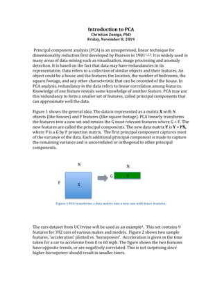
Figure
1
shows
the
general
idea.
The
data
is
represented
as
a
matrix
X
with
N
objects
(like
houses)
and
F
features
(like
square
footage).
PCA
linearly
transforms
the
features
into
a
new
set
and
retains
the
G
most
relevant
features
where
G
<
F.
The
new
features
are
called
the
principal
components.
The
new
data
matrix
Y
is
Y
=
PX,
where
P
is
a
G
by
F
projection
matrix.
The
first
principal
component
captures
most
of
the
variance
of
the
data.
Each
additional
principal
component
is
made
to
capture
the
remaining
variance
and
is
uncorrelated
or
orthogonal
to
other
principal
components.
Figure
1
PCA
transforms
a
data
matrix
into
a
new
one
with
fewer
features.
The
cars
dataset
from
UC
Irvine
will
be
used
as
an
example4.
This
set
contains
9
features
for
392
cars
of
various
makes
and
models.
Figure
2
shows
two
sample
features,
‘acceleration’
plotted
vs.
‘horsepower’.
Acceleration
is
given
in
the
time
taken
for
a
car
to
accelerate
from
0
to
60
mph.
The
figure
shows
the
two
features
have
opposite
trends,
or
are
negatively
correlated.
This
is
not
surprising
since
higher
horsepower
should
result
in
smaller
times.
2.
Figure
2
Two
features
of
car
data
set
shows
the
data
is
concentrated
along
a
line
P1.
Figure
2
shows
that
most
of
the
variation
of
the
features
is
concentrated
along
a
line
labeled
‘P1’.
The
remainder
of
the
variation
is
along
a
second
line
labeled
‘P2’.
The
lines
can
be
characterized
by
unit
vectors
vj
=
[a1j,
a2j]
(j=1,2)
that
give
the
lines’
orientations.
The
lines’
displacements
from
the
origin
do
not
matter
since
the
data
will
later
be
centered
at
zero.
Each
point
represents
a
car
and
can
also
be
represented
by
a
vector
xi
=
[horsepoweri,
accelerationi],
where
the
subscript
corresponds
to
the
ith
car.
Each
point
can
be
projected
onto
a
line
Pj
by
the
inner
product
of
vj
and
xi
as
shown
in
Figure
3.
𝑝!" = 𝑎!! 𝑎𝑐𝑐𝑒𝑙𝑒𝑟𝑎𝑡𝑖𝑜𝑛! + 𝑎!!ℎ𝑜𝑟𝑠𝑒𝑝𝑜𝑤𝑒𝑟!
Figure
3
Projecting
a
point
onto
line
P1.
This
new
feature
p1
is
the
first
principal
component
and
is
a
linear
combination
of
the
original
two
features,
horsepower
and
acceleration.
In
general
it
will
not
have
a
more
descriptive
name
but
one
could
be
given
to
clarify
the
concept.
One
option
is
to
think
of
the
combination
of
‘horsepower’
and
‘acceleration’
as
the
‘performance’
of
the
car.
3. The
question
is
then
how
to
find
the
coefficients
a11,
and
a21
of
vector
v1,
which
gives
the
direction
of
the
best-‐fit
line
P1.
This
line
should
be
as
close
to
all
points
as
possible,
minimizing
the
average
distance
J
to
all
the
points.
𝐽 =
1
𝑁
𝑑!
!
!
!!!
The
solution
lies
in
the
covariance
matrix
of
the
features
SX.
Specifically;
the
eigenvectors
of
SX
give
the
required
vectors
v1
and
v2.
To
calculate
the
covariance
matrix,
the
mean
of
each
feature
is
subtracted
from
each
row.
To
put
the
features
on
a
similar
scale,
they
should
also
be
divided
by
their
standard
deviation.
This
is
done
to
prevent
the
analysis
from
capturing
uninteresting
directions
in
the
data.
After
this
preprocessing
of
the
data
matrix
X,
the
covariance
matrix
is
and
F
by
F
matrix:
𝑺! =
1
𝑁
𝑿𝑿!
The
vector
v1
corresponds
to
the
eigenvector
with
largest
eigenvalue
λM.
Vector
v1
corresponds
to
the
second
smaller
eigenvalue
λm
(λm
<
λM).
𝑺 𝑿 𝒗 𝟏 = 𝜆! 𝒗 𝟏
𝑺 𝑿 𝒗 𝟐 = 𝜆! 𝒗 𝟐
For
the
car
data
set,
using
only
the
features
‘acceleration’
and
‘horsepower’,
the
covariance
matrix
is.
𝑺 𝑿 =
1 −0.69
−0.69 1
The
off-‐diagonal
term
-‐0.69
shows
the
cross-‐covariance
between
horsepower
and
acceleration,
which
is
negative
as
implied
by
Figure
1.
The
diagonal
terms
show
the
auto-‐covariance
of
each
feature
and
have
value
1
because
of
the
pre-‐scaling.
Using
any
linear
algebra
solver
readily
gives
the
eigenvectors
of
the
covariance
matrix.
The
eigenvalues
are
(1.69,
0.31).
Their
sum
is
the
total
variance,
which
is
2.
Vector
v1
is
[0.707,
-‐0.707]
and
captures
84.5%
of
the
total
variance
(1.69/2).
Figure
4
shows
the
resulting
directions
of
v1
and
v2.
4.
Figure
4
Rescaled
data
with
the
direction
of
the
2
principal
components.
The
projection
matrix
P
can
be
made
with
v1
and
v2
as
rows.
If
both
vectors
are
kept,
there
is
no
loss
in
representation.
The
new
representation
would
have
a
covariance
matrix.
𝑺! =
1
𝑁
𝒀𝒀!
𝑺! =
1
𝑁
𝑷𝑿 𝑷𝑿 !
= 𝑷𝑺 𝑿 𝑷!
= 𝚲
Since
P
has
the
eigenvectors
of
Sx
as
rows,
the
right
hand
side
results
in
a
diagonal
matrix
of
the
eigenvalues
of
Sx.
𝑆! =
1.69 0
0 0.31
For
dimensionality
reduction,
only
v1
would
be
used.
The
new
representation,
matrix
Y,
would
have
a
single
feature,
the
first
principle
component
(Y
=
v1X).
PCA
can
be
applied
to
any
number
of
features.
The
car
data
set
has
the
additional
features:
‘cylinders’,
‘displacement’,
and
‘weight’
for
a
total
of
5
features.
Other
features
are
categorical
and
one
‘mpg’
is
usually
the
target
variable
of
interest.
The
same
process
can
be
done
to
obtain
the
principal
components.
Each
principal
component
is
a
linear
combination
of
these
5
features.
Standard
scaling
is
applied
on
the
features
before
making
the
covariance
matrix
Sx
(now
a
5
by
5
matrix).
The
eigenvalues
and
eigenvectors
are
found
and
the
eigenvectors
used
to
make
the
projection
matrix
P.
Figure
5
shows
the
percentage
of
variance
explained
by
each
component.
Again
the
first
component
captures
over
80%
of
the
total
variance.
Instead
of
5
features,
1-‐2
principal
components
may
be
enough
for
various
purposes.
5.
Figure
5
Percentage
of
variance
explained
by
each
principal
component.
For
example,
Figure
6
shows
a
plot
of
principal
component
2
vs.
principal
component
1.
Together
they
capture
about
96%
of
the
total
variance.
The
figure
shows
there
may
be
3
clusters,
or
groups
of
cars.
These
may
correspond
to
different
types
of
cars
such
as
sports
cars,
sedans,
and
trucks.
Confirming
with
the
make
of
the
car
might
clarify
this.
A
clustering
algorithm
like
k-‐means
may
be
applied
to
quantify
the
clusters.
This
shows
a
common
application
of
PCA
in
dimensionality
reduction
where
fewer
features
help
with
many
machine
learning
algorithms.
Figure
6
Principal
Component
2
vs.
1
indicates
there
may
be
around
3
clusters.
To
summarize,
PCA
is
a
linear,
dimensionality
reduction
technique
that
forms
new
features
using
linear
combinations
of
the
original.
These
new
features,
the
principal
components,
maximize
the
total
variance
capture
and
are
uncorrelated
with
each
other.
The
eigenvectors
of
the
covariance
matrix
are
used
to
transform
the
data
matrix.
In
practice
if
there
are
many
features,
forming
the
covariance
matrix
may
be
computationally
expensive
and
an
SVD
of
the
data
matrix
is
used.
[1]
Gilbert
Strang
“Linear
Algebra
and
Learning
from
Data”
Wellesley
Cambridge
Press
2019
6. [2]
Deisenroth,
et.
Al.
“Mathematics
for
Machine
Learning”
to
be
published
Cambridge
University
Press.
https://mml-‐book.com
[3]
Shlens
“A
Tutorial
on
Principal
Component
Analysis”
2014
https://arxiv.org/abs/1404.1100
[4]
https://archive.ics.uci.edu/ml/datasets/car+evaluation
![Figure
2
Two
features
of
car
data
set
shows
the
data
is
concentrated
along
a
line
P1.
Figure
2
shows
that
most
of
the
variation
of
the
features
is
concentrated
along
a
line
labeled
‘P1’.
The
remainder
of
the
variation
is
along
a
second
line
labeled
‘P2’.
The
lines
can
be
characterized
by
unit
vectors
vj
=
[a1j,
a2j]
(j=1,2)
that
give
the
lines’
orientations.
The
lines’
displacements
from
the
origin
do
not
matter
since
the
data
will
later
be
centered
at
zero.
Each
point
represents
a
car
and
can
also
be
represented
by
a
vector
xi
=
[horsepoweri,
accelerationi],
where
the
subscript
corresponds
to
the
ith
car.
Each
point
can
be
projected
onto
a
line
Pj
by
the
inner
product
of
vj
and
xi
as
shown
in
Figure
3.
𝑝!" = 𝑎!! 𝑎𝑐𝑐𝑒𝑙𝑒𝑟𝑎𝑡𝑖𝑜𝑛! + 𝑎!!ℎ𝑜𝑟𝑠𝑒𝑝𝑜𝑤𝑒𝑟!
Figure
3
Projecting
a
point
onto
line
P1.
This
new
feature
p1
is
the
first
principal
component
and
is
a
linear
combination
of
the
original
two
features,
horsepower
and
acceleration.
In
general
it
will
not
have
a
more
descriptive
name
but
one
could
be
given
to
clarify
the
concept.
One
option
is
to
think
of
the
combination
of
‘horsepower’
and
‘acceleration’
as
the
‘performance’
of
the
car.](data:image/gif;base64,R0lGODlhAQABAIAAAAAAAP///yH5BAEAAAAALAAAAAABAAEAAAIBRAA7)