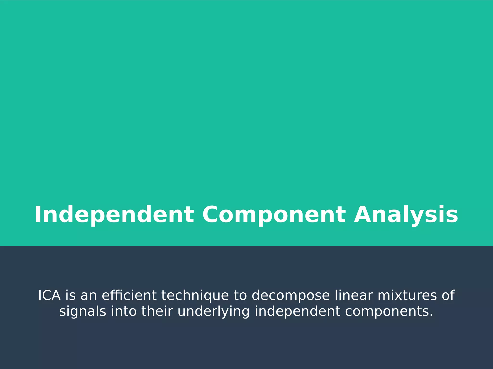
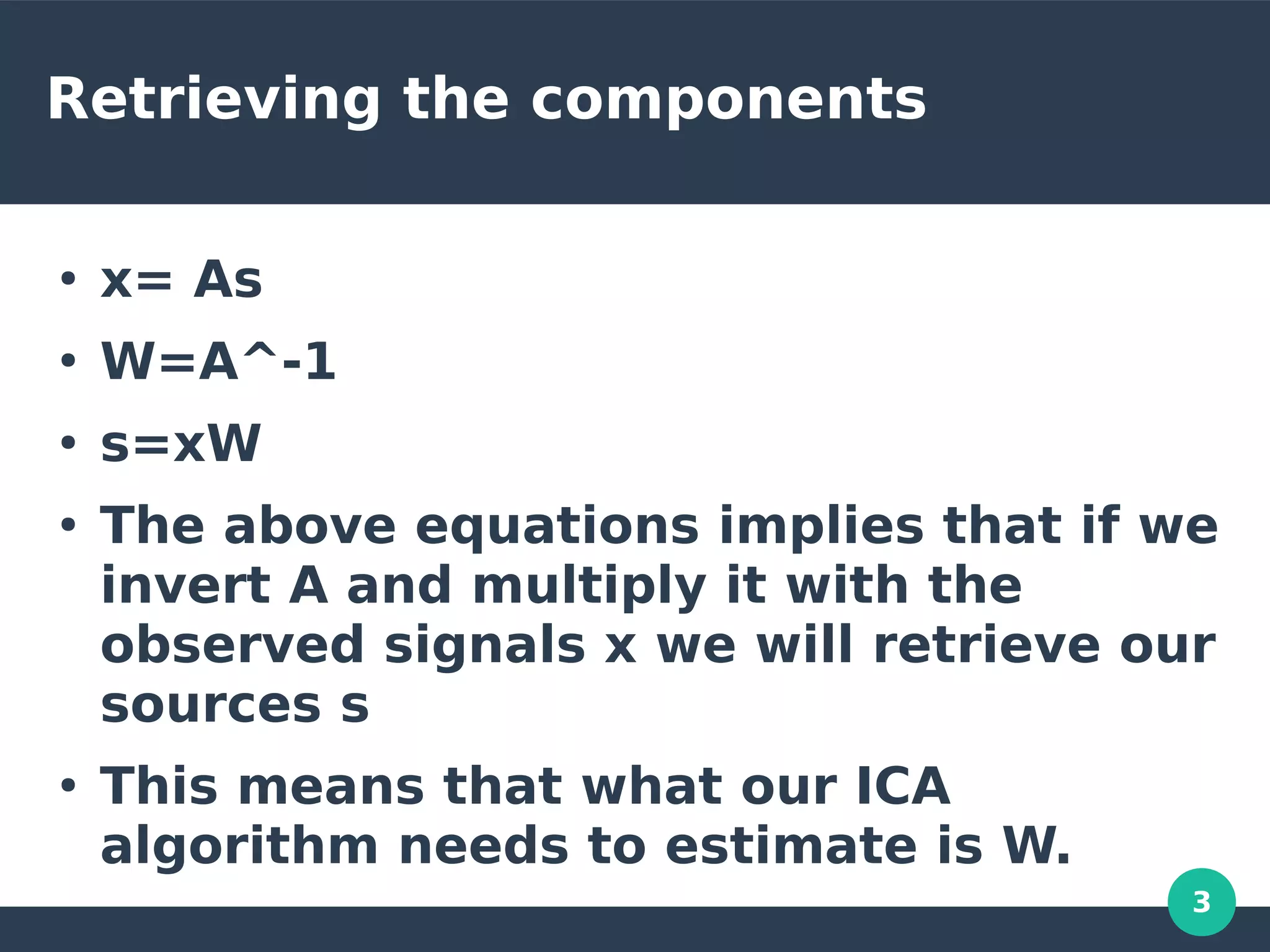
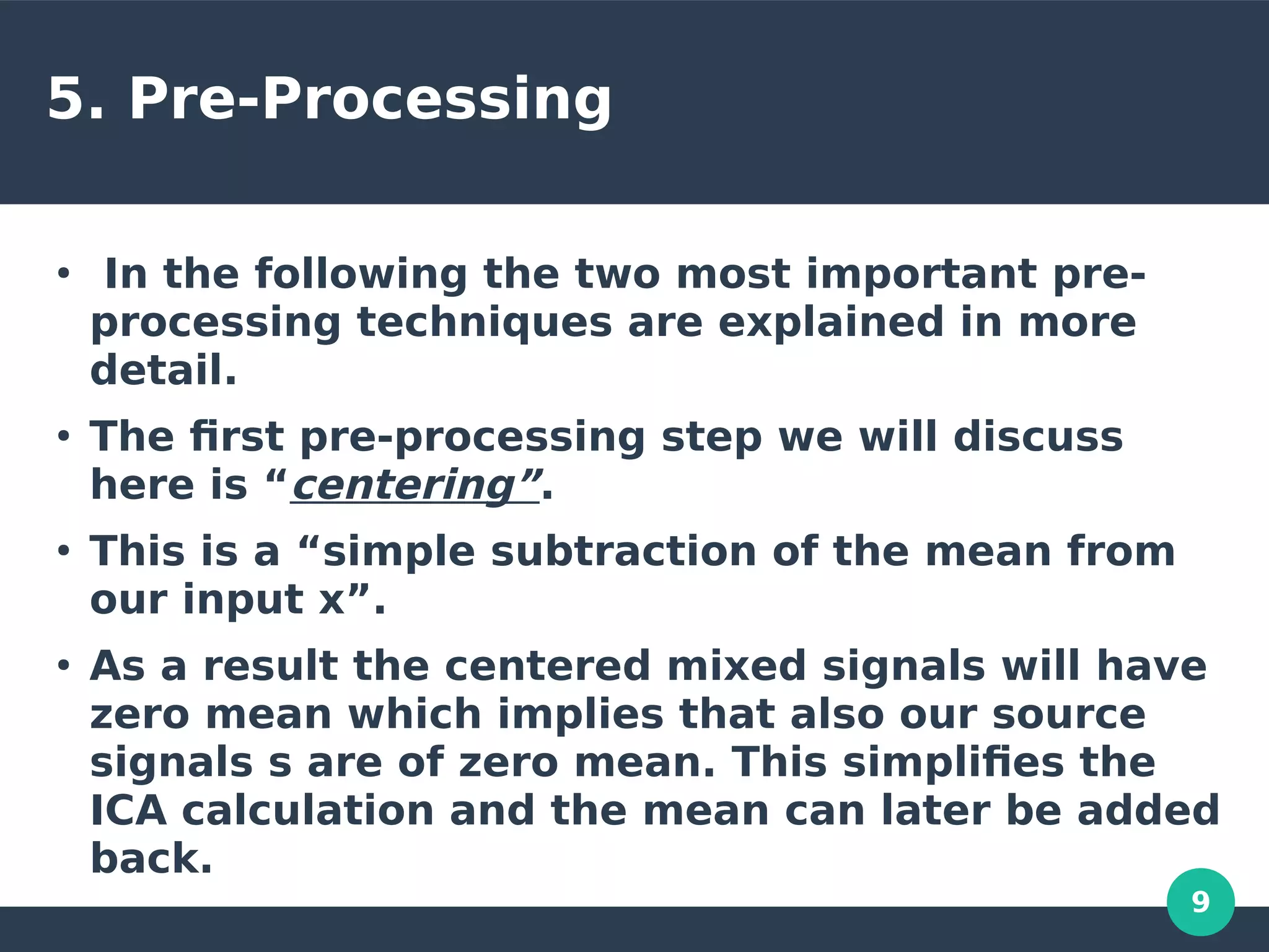
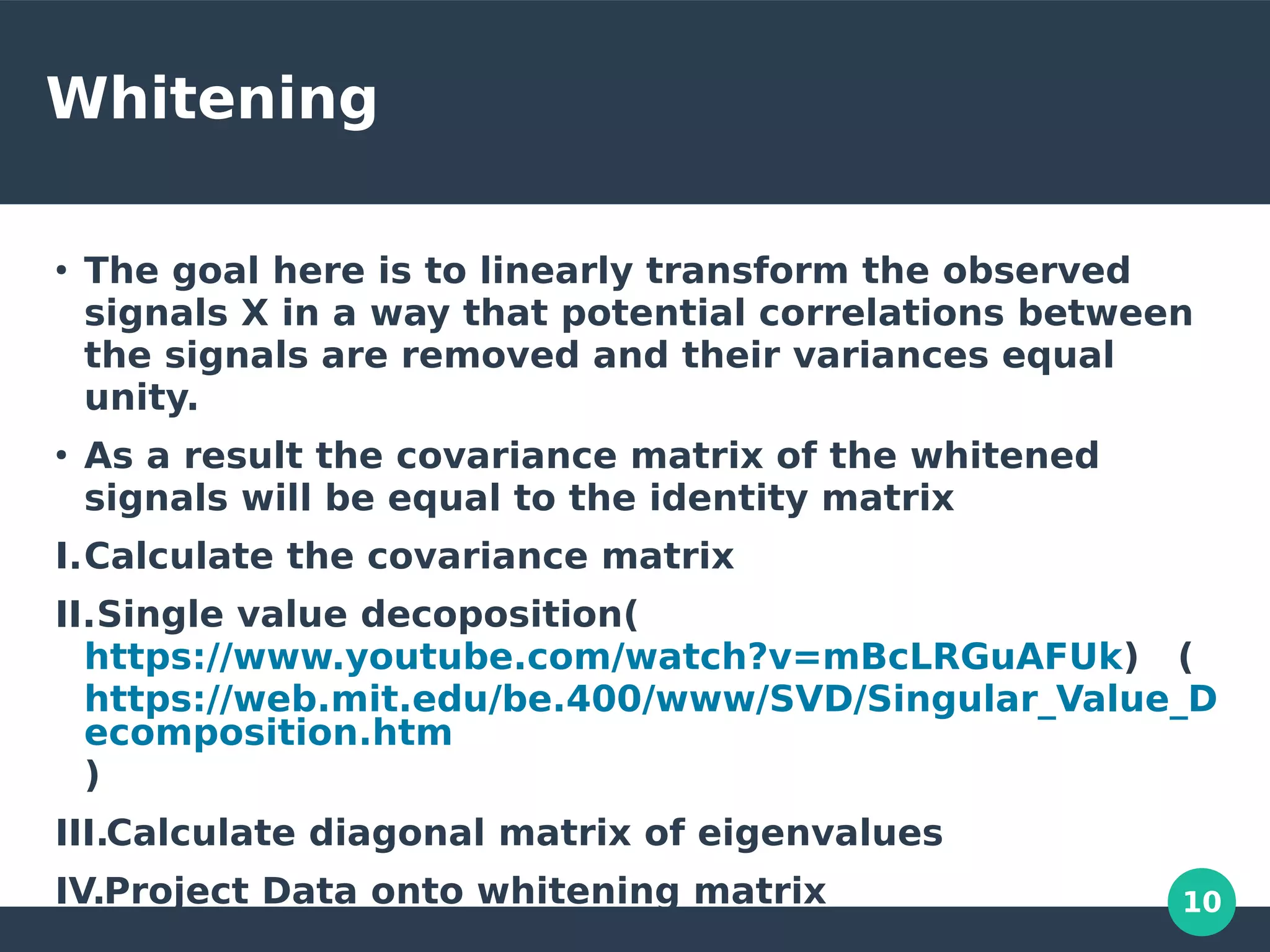
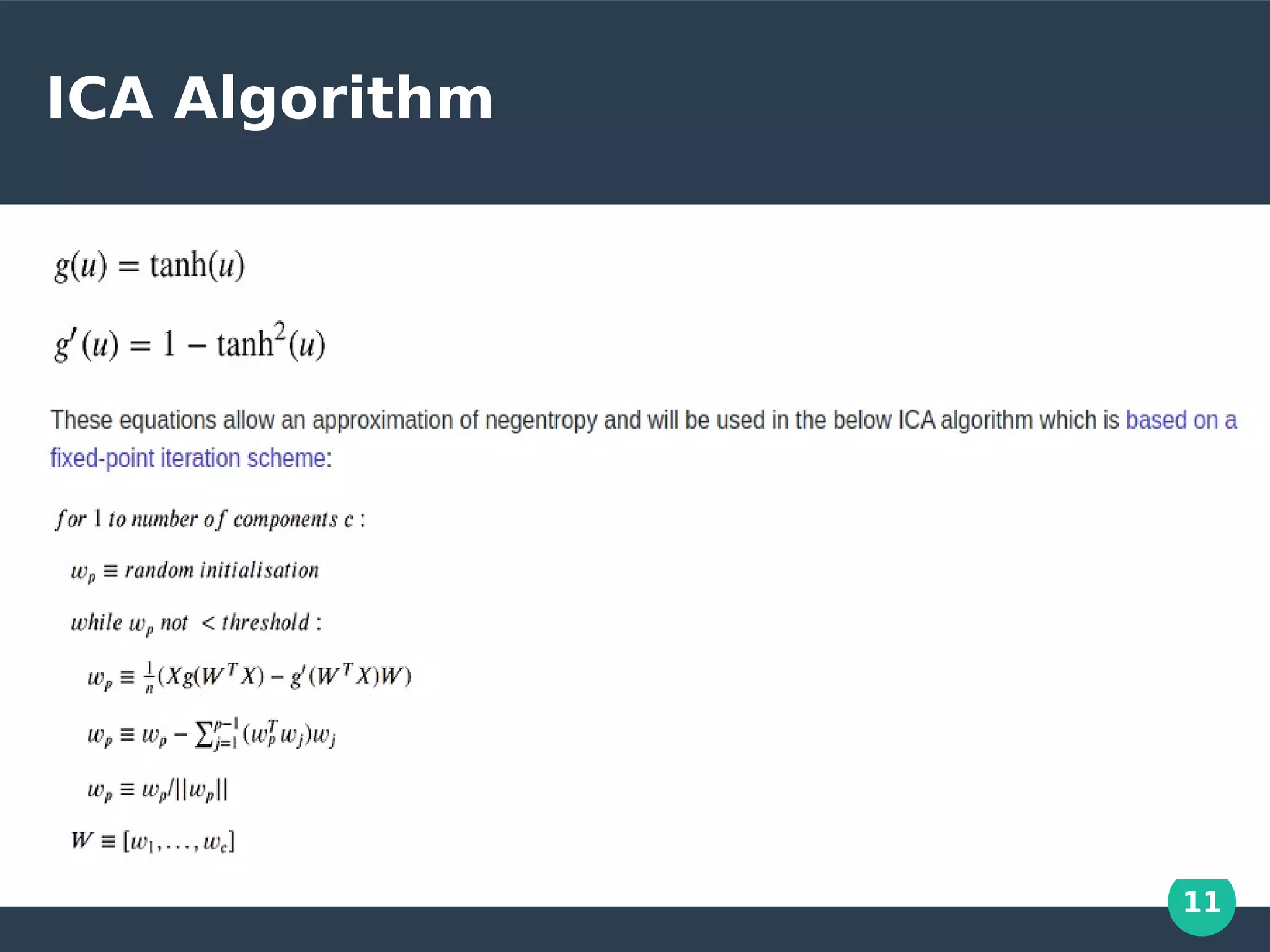
This document provides an overview of Independent Component Analysis (ICA). It discusses: 1. ICA is a technique that decomposes linear mixtures of signals into their underlying independent components. 2. The ICA model assumes observed data is generated by some independent source signals that are linearly combined using a mixing matrix. ICA estimates the inverse of this mixing matrix to retrieve the original source signals. 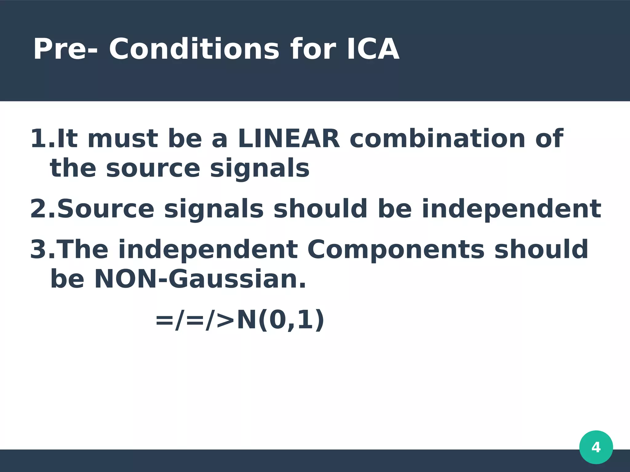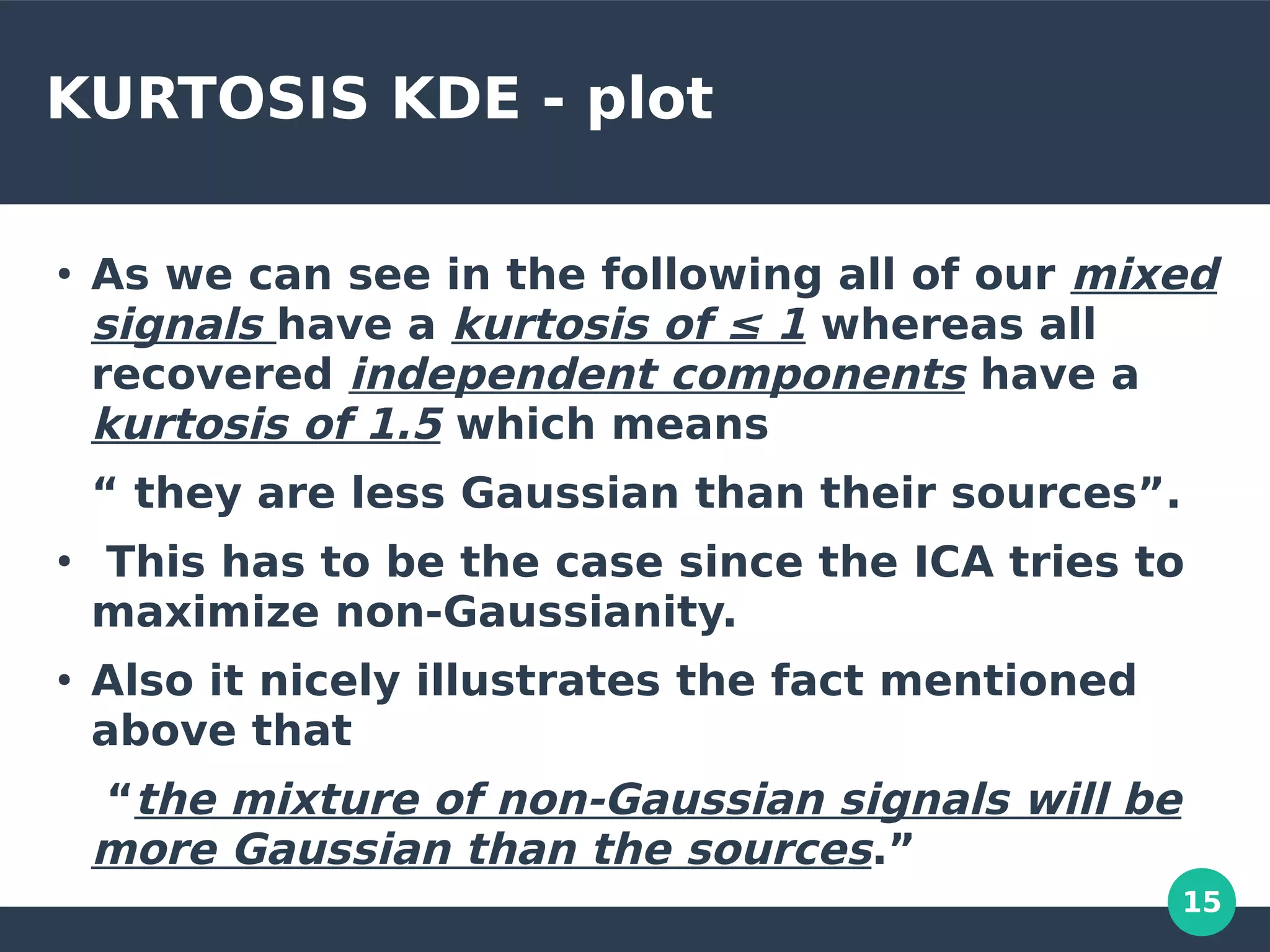3. For ICA to work, the source signals must be independent and non-Gaussian. The document demonstrates ICA on some toy signals and verifies the recovered components match this criteria.

1. Independent Component Analysis
ICA is an efficient technique to decompose linear mixtures of
signals into their underlying independent components.

2. 2
The generative model of ICA
●
The ICA is based on a generative model.
This means that it assumes an underlying
process that generates the observed
data. The ICA model is simple, it assumes
that some independent source signals s
are linear combined by a mixing matrix A.
●
x=As
●
x=Observed Signal Matrix
●
A=Mixing matrix
●
s=source signals

3. 3
Retrieving the components
●
x= As
●
W=A^-1
●
s=xW
●
The above equations implies that if we
invert A and multiply it with the
observed signals x we will retrieve our
sources s
●
This means that what our ICA
algorithm needs to estimate is W.

4. 4
Pre- Conditions for ICA
1.It must be a LINEAR combination of
the source signals
2.Source signals should be independent
3.The independent Components should
be NON-Gaussian.
=/=/>N(0,1)

5. 5
1. Independent Sources
●
The independent sources signals(s)
are
●
(1) a sine wave
●
(2) a saw tooth signal
●
(3) a random noise vector.
●
After calculating their dot product
with A we get three linear
combinations of these source signals.

6. 6
2. Plotting
●
A Plot of the 3 Independent Sources is
done .
●
The 3 observed Mixed signals are also
plotted
●
To verify the observation and to
understand the existing nature of one
signal on the other through visual
representation

7. 7
Gaussian Vs Non-Gaussian
●
Differences between Gaussian and non-Gaussian
signals
●
The joint density distribution of two independent non-
Gaussian signals will be uniform on a square. Mixing
these two signals with an orthogonal matrix will result
in two signals that are now not independent anymore
and have a uniform distribution on a parallelogram
●
Central Limit Theorem: The central limit theorem
states that if you have a population with mean μ and
standard deviation σ and take sufficiently large
random samples from the population with
replacement , then the distribution of the sample
means will be approximately normally distributed.

8. 8
4. Scatter Plot
●
For better visualisation the scatter plot is
plotted for the Source signals and mixed signals
●
To check if the properties discussed in the
previous slide also apply for our toy signals we
will plot them accordingly.
●
As expected the source signals are distributed
on a square for non-Gaussian random variables.
●
Likewise the mixed signals form a parallelogram
in the right plot of Figure 3 which shows that
the mixed signals are not independent
anymore.

9. 9
5. Pre-Processing
●
In the following the two most important pre-
processing techniques are explained in more
detail.
●
The first pre-processing step we will discuss
here is “centering”.
●
This is a “simple subtraction of the mean from
our input x”.
●
As a result the centered mixed signals will have
zero mean which implies that also our source
signals s are of zero mean. This simplifies the
ICA calculation and the mean can later be added
back.

10. 10
Whitening
●
The goal here is to linearly transform the observed
signals X in a way that potential correlations between
the signals are removed and their variances equal
unity.
●
As a result the covariance matrix of the whitened
signals will be equal to the identity matrix
I.Calculate the covariance matrix
II.Single value decoposition(
https://www.youtube.com/watch?v=mBcLRGuAFUk) (
https://web.mit.edu/be.400/www/SVD/Singular_Value_D
ecomposition.htm
)
III.Calculate diagonal matrix of eigenvalues
IV.Project Data onto whitening matrix

11. 11
ICA Algorithm

12. 12
The math explained
●
So according to the above what we have to do is to take a random
guess for the weights of each component.
●
The dot product of the random weights and the mixed signals is
passed into the two functions g and g'.
●
We then subtract the result of g' from g and calculate the mean.
The result is our new weights vector.
●
Next we could directly divide the new weights vector by its norm
and repeat the above until the weights do not change anymore.
●
There would be nothing wrong with that. However the problem we
are facing here is that in the iteration for the second component
we might identify the same component as in the first iteration.
●
To solve this problem we have to decorrelate the new weights
from the previously identified weights.
●
This is what is happening in the step between updating the
weights and dividing by their norm.

13. 13
Running the functions
●
We now run through the pre-
processing steps.
●
Run the ICA algorithm designed
●
Observe the plot

14. 14
KURTOSIS
●
Kurtosis is the fourth moment of the data
and measures the "tailedness" of a
distribution.
●
The first moment is the mean, the second is
the variance, the third is the skewness and
the fourth is the kurtosis.
●
Here 3 is subtracted from the fourth
moment so that a normal distribution has a
kurtosis of 0.
●
KURTOSIS 0 INDICATES PERFECT GAUSSIAN
OR NORMAL DISTRIBUTION.

15. 15
KURTOSIS KDE - plot
●
As we can see in the following all of our mixed
signals have a kurtosis of ≤ 1 whereas all
recovered independent components have a
kurtosis of 1.5 which means
“ they are less Gaussian than their sources”.
●
This has to be the case since the ICA tries to
maximize non-Gaussianity.
●
Also it nicely illustrates the fact mentioned
above that
“the mixture of non-Gaussian signals will be
more Gaussian than the sources.”

16. 16
ICA -SKlearn
●
The implementation of ICA from
sklearn is well optimized.
●
It is more efficient than Induvidually
programming the math into code.
●
Less time requirement to both process
and code and it’s self explanatory
●
We shall see it in action.

17. 17
Beautiful Example Comparing
methods

18. 18
Thank You!