Tutorials questions

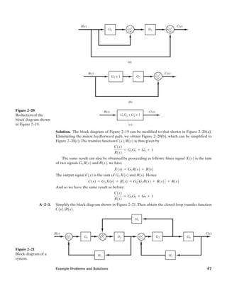
Example Problems and Solutions 47
G1 G2
R(s) C(s)
G2
R(s) C(s)
G1 + 1
R(s) C(s)
G1G2 + G2 + 1
(a)
(b)
(c)
+
+
+
+
+
+
Figure 2–20
Reduction of the
block diagram shown
in Figure 2–19.
Solution. The block diagram of Figure 2–19 can be modified to that shown in Figure 2–20(a).
Eliminating the minor feedforward path, we obtain Figure 2–20(b), which can be simplified to
Figure 2–20(c).The transfer function C(s)/R(s) is thus given by
The same result can also be obtained by proceeding as follows: Since signal X(s) is the sum
of two signals G1R(s) and R(s), we have
The output signal C(s) is the sum of G2X(s) and R(s). Hence
And so we have the same result as before:
A–2–3. Simplify the block diagram shown in Figure 2–21. Then obtain the closed-loop transfer function
C(s)/R(s).
C(s)
R(s)
= G1G2 + G2 + 1
C(s) = G2X(s) + R(s) = G2 CG1R(s) + R(s)D + R(s)
X(s) = G1R(s) + R(s)
C(s)
R(s)
= G1G2 + G2 + 1
G1 G2
H3
G3 G4
H2H1
+
–
+
+ +
–
R(s) C(s)
Figure 2–21
Block diagram of a
system.

48 Chapter 2 / Mathematical Modeling of Control Systems
G1
G1
G2
H3
G4
G3 G4
H2H1
+
+
+
+
+
–
+
–
R(s)
R(s) C(s)
C(s)
H3
G1G4
G1 G2
1 + G1 G2 H1
R(s) C(s)G1 G2 G3 G4
1+ G1 G2 H1 + G3 G4 H2 – G2 G3 H3 + G1 G2 G3 G4 H1 H2
G3 G4
1 + G3 G4 H2
1
(a)
(b)
(c)
Figure 2–22
Successive
reductions of the
block diagram shown
in Figure 2–21.
G1
Gp
+
+
+
–
+
+
Gf
C(s)
D(s)
R(s) E(s) U(s)
H
Gc
Figure 2–23
Control system with
reference input and
disturbance input.
Solution. First move the branch point between G3 and G4 to the right-hand side of the loop con-
taining G3, G4, and H2. Then move the summing point between G1 and G2 to the left-hand side
of the first summing point. See Figure 2–22(a). By simplifying each loop, the block diagram can
be modified as shown in Figure 2–22(b). Further simplification results in Figure 2–22(c), from
which the closed-loop transfer function C(s)/R(s) is obtained as
A–2–4. Obtain transfer functions C(s)/R(s) and C(s)/D(s) of the system shown in Figure 2–23.
Solution. From Figure 2–23 we have
(2–47)
(2–48)
(2–49)E(s) = R(s) - HC(s)
C(s) = Gp CD(s) + G1U(s)D
U(s) = GfR(s) + GcE(s)
C(s)
R(s)
=
G1G2G3G4
1 + G1G2H1 + G3G4H2 - G2G3H3 + G1G2G3G4H1H2

By substituting Equation (2–47) into Equation (2–48), we get
(2–50)
By substituting Equation (2–49) into Equation (2–50), we obtain
Solving this last equation for C(s), we get
Hence
(2–51)
Note that Equation (2–51) gives the response C(s) when both reference input R(s) and distur-
bance input D(s) are present.
To find transfer function C(s)/R(s), we let D(s)=0 in Equation (2–51).Then we obtain
Similarly, to obtain transfer function C(s)/D(s), we let R(s)=0 in Equation (2–51). Then
C(s)/D(s) can be given by
A–2–5. Figure 2–24 shows a system with two inputs and two outputs. Derive C1(s)/R1(s), C1(s)/R2(s),
C2(s)/R1(s), and C2(s)/R2(s). (In deriving outputs for R1(s), assume that R2(s) is zero, and vice
versa.)
C(s)
D(s)
=
Gp
1 + G1GpGcH
C(s)
R(s)
=
G1GpAGf + GcB
1 + G1GpGcH
C(s) =
GpD(s) + G1GpAGf + GcBR(s)
1 + G1GpGcH
C(s) + G1GpGcHC(s) = GpD(s) + G1GpAGf + GcBR(s)
C(s) = GpD(s) + G1Gp EGfR(s) + Gc CR(s) - HC(s)D F
C(s) = GpD(s) + G1Gp CGfR(s) + GcE(s)D
G1
C1
C2
R1
R2
G3
G4
+
−
+
−
G2
Figure 2–24
System with two
inputs and two
outputs.

Solution. From the figure, we obtain
(2–52)
(2–53)
(2–54)
By substituting Equation (2–52) into Equation (2–53), we get
(2–55)
Solving Equation (2–54) for C1, we obtain
(2–56)
Solving Equation (2–55) for C2 gives
(2–57)
Equations (2–56) and (2–57) can be combined in the form of the transfer matrix as follows:
Then the transfer functions C1(s)/R1(s), C1(s)/R2(s), C2(s)/R1(s) and C2(s)/R2(s) can be obtained
as follows:
Note that Equations (2–56) and (2–57) give responses C1 and C2, respectively, when both inputs
R1 and R2 are present.
Notice that when R2(s)=0, the original block diagram can be simplified to those shown in
Figures 2–25(a) and (b). Similarly, when R1(s)=0, the original block diagram can be simplified
to those shown in Figures 2–25(c) and (d). From these simplified block diagrams we can also ob-
tain C1(s)/R1(s), C2(s)/R1(s), C1(s)/R2(s), and C2(s)/R2(s), as shown to the right of each corre-
sponding block diagram.
C2(s)
R1(s)
= -
G1G2G4
1 - G1G2G3G4
,
C2(s)
R2(s)
=
G4
1 - G1G2G3G4
C1(s)
R1(s)
=
G1
1 - G1G2G3G4
,
C1(s)
R2(s)
= -
G1G3G4
1 - G1G2G3G4
B
C1
C2
R = D
G1
1 - G1G2G3G4
-
G1G2G4
1 - G1G2G3G4
-
G1G3G4
1 - G1G2G3G4
G4
1 - G1G2G3G4
T B
R1
R2
R
C2 =
-G1G2G4R1 + G4R2
1 - G1G2G3G4
C1 =
G1R1 - G1G3G4R2
1 - G1G2G3G4
C2 = G4 CR2 - G2G1AR1 - G3C2BD
C1 = G1 CR1 - G3G4AR2 - G2C1BD
C2 = G4AR2 - G2C1B
C1 = G1AR1 - G3C2B

Thus
Hence a linear approximation of the given nonlinear equation near the operating point is
z - 30x - 72y + 243 = 0
z - 243 = 30(x - 9) + 72(y - 3)
R(s) C(s)
G1 G2 G3
H1
H2
H3
+
–
+
–
+
–
+
+
Figure 2–31
Block diagram of a system.
B–2–1. Simplify the block diagram shown in Figure 2–29
and obtain the closed-loop transfer function C(s)/R(s).
PROBLEMS
R(s) C(s)
G1
G2
G3
G4
+
–
+
–
+
+
Figure 2–29
R(s) C(s)
G1
G2
H1
H2
+
–
+
+
+
–
Figure 2–30

86 Chapter 3 / Mathematical Modeling of Mechanical Systems and Electrical Systems
EXAMPLE PROBLEMS AND SOLUTIONS
A–3–1. Figure 3–20(a) shows a schematic diagram of an automobile suspension system.As the car moves
along the road, the vertical displacements at the tires act as the motion excitation to the auto-
mobile suspension system.The motion of this system consists of a translational motion of the cen-
ter of mass and a rotational motion about the center of mass. Mathematical modeling of the
complete system is quite complicated.
A very simplified version of the suspension system is shown in Figure 3–20(b).Assuming that
the motion xi at point P is the input to the system and the vertical motion xo of the body is the
output,obtain the transfer function (Consider the motion of the body only in the ver-
tical direction.) Displacement xo is measured from the equilibrium position in the absence of
input xi.
Solution. The equation of motion for the system shown in Figure 3–20(b) is
or
Taking the Laplace transform of this last equation, assuming zero initial conditions, we obtain
Hence the transfer function Xo(s)/Xi(s) is given by
Xo(s)
Xi(s)
=
bs + k
ms2
+ bs + k
Ams2
+ bs + kBXo(s) = (bs + k)Xi(s)
mx
$
o + bx
#
o + kxo = bxi
#
+ kxi
mx
$
o + bAx
#
o - x
#
iB + kAxo - xiB = 0
Xo(s)͞Xi(s).
(a)
k
(b)
xi
Center of mass
Auto body
b
P
xo
m
Figure 3–20
(a) Automobile
suspension system;
(b) simplified
suspension system.

A–3–2. Obtain the transfer function Y(s)/U(s) of the system shown in Figure 3–21. The input u is a
displacement input. (Like the system of Problem A–3–1, this is also a simplified version of an
automobile or motorcycle suspension system.)
Solution. Assume that displacements x and y are measured from respective steady-state
positions in the absence of the input u. Applying the Newton’s second law to this system, we
obtain
Hence, we have
Taking Laplace transforms of these two equations, assuming zero initial conditions, we obtain
Eliminating X(s) from the last two equations, we have
which yields
Y(s)
U(s)
=
k1Abs + k2B
m1m2s4
+ Am1 + m2Bbs3
+ Ck1m2 + Am1 + m2Bk2 Ds2
+ k1bs + k1k2
Am1s2
+ bs + k1 + k2B
m2s2
+ bs + k2
bs + k2
Y(s) = Abs + k2BY(s) + k1U(s)
Cm2s2
+ bs + k2 DY(s) = Abs + k2BX(s)
Cm1s2
+ bs + Ak1 + k2BDX(s) = Abs + k2BY(s) + k1U(s)
m2y
$
+ by
#
+ k2y = bx
#
+ k2x
m1x
$
+ bx
#
+ Ak1 + k2Bx = by
#
+ k2y + k1u
m2y
$
= -k2(y - x) - b(y
#
- x
#
)
m1x
$
= k2(y - x) + b(y
#
- x
#
) + k1(u - x)
y
b
x
u
m2
m1
k2
k1
Figure 3–21
Suspension system.

A–3–3. Obtain a state-space representation of the system shown in Figure 3–22.
Solution. The system equations are
The output variables for this system are y1 and y2. Define state variables as
Then we obtain the following equations:
Hence, the state equation is
and the output equation is
A–3–4. Obtain the transfer function Xo(s)/Xi(s) of the mechanical system shown in Figure 3–23(a). Also
obtain the transfer function Eo(s)/Ei(s) of the electrical system shown in Figure 3–23(b). Show that
these transfer functions of the two systems are of identical form and thus they are analogous systems.
B
y1
y2
R = B
1
0
0
0
0
1
0
0
R D
x1
x2
x3
x4
T
D
x
#
1
x
#
2
x
#
3
x
#
4
T = F
0
-
k
m1
0
k
m2
1
-
b
m1
0
0
0
k
m1
0
-
k
m2
0
0
1
0
V D
x1
x2
x3
x4
T + E
0
0
0
1
m2
U u
x
#
4 =
1
m2
C-kAy2 - y1B + uD =
k
m2
x1 -
k
m2
x3 +
1
m2
u
x
#
3 = x4
x
#
2 =
1
m1
C-by
#
1 - kAy1 - y2B D = -
k
m1
x1 -
b
m1
x2 +
k
m1
x3
x
#
1 = x2
x4 = y
#
2
x3 = y2
x2 = y
#
1
x1 = y1
m2y
$
2 + kAy2 - y1B = u
m1y
$
1 + by
#
1 + kAy1 - y2B = 0
m1 m2
k
y1
b
u
y2
Figure 3–22
Mechanical system.

Solution. In Figure 3–23(a) we assume that displacements xi, xo, and y are measured from their
respective steady-state positions.Then the equations of motion for the mechanical system shown
in Figure 3–23(a) are
By taking the Laplace transforms of these two equations,assuming zero initial conditions,we have
If we eliminate Y(s) from the last two equations, then we obtain
or
Hence the transfer function Xo(s)/Xi(s) can be obtained as
For the electrical system shown in Figure 3–23(b), the transfer function Eo(s)/Ei(s) is found to be
=
AR1C1s + 1BAR2C2s + 1B
AR1C1s + 1BAR2C2s + 1B + R2C1s
Eo(s)
Ei(s)
=
R1 +
1
C1s
1
A1͞R2B + C2s
+ R1 +
1
C1s
Xo(s)
Xi(s)
=
a
b1
k1
s + 1b a
b2
k2
s + 1b
a
b1
k1
s + 1b a
b2
k2
s + 1 b +
b2
k1
s
Ab1s + k1BXi(s) = a b1s + k1 + b2s - b2s
b2s
b2s + k2
b Xo(s)
b1 CsXi(s) - sXo(s)D + k1 CXi(s) - Xo(s)D = b2sXo(s) - b2s
b2sXo(s)
b2s + k2
b2 CsXo(s) - sY(s)D = k2Y(s)
b1 CsXi(s) - sXo(s)D + k1 CXi(s) - Xo(s)D = b2 CsXo(s) - sY(s)D
b2Ax
#
o - y
#
B = k2y
b1Ax
#
i - x
#
oB + k1Axi - xoB = b2Ax
#
o - y
#
B
(a) (b)
xi
xo
yk2
k1
b2
b1
R2
R1
eoei
C2
C1
Figure 3–23
(a) Mechanical
system;
(b) analogous
electrical system.

A–3–8. Obtain the transfer function of the operational-amplifier circuit shown in Figure 3–28.
Solution. We will first obtain currents i1, i2, i3, i4, and i5.Then we will use node equations at nodes
A and B.
At node A, we have i1=i2+i3+i4, or
(3–42)
At node B, we get i4=i5, or
(3–43)
By rewriting Equation (3–42), we have
(3–44)
From Equation (3–43), we get
(3–45)
Taking the Laplace transform of this last equation, assuming zero initial conditions, we obtain
from which we get the transfer function as follows:
Eo(s)
Ei(s)
= -
1
R1C1R2C2s2
+ CR2C2 + R1C2 + AR1͞R3BR2C2 Ds + AR1͞R3B
Eo(s)͞Ei(s)
-C1C2R2s2
Eo(s) + a
1
R1
+
1
R2
+
1
R3
b A-R2C2BsEo(s) -
1
R3
Eo(s) =
Ei(s)
R1
C1 a -R2C2
d2
eo
dt2
b + a
1
R1
+
1
R2
+
1
R3
b A-R2C2B
deo
dt
=
ei
R1
+
eo
R3
eA = -R2C2
deo
dt
C1
deA
dt
+ a
1
R1
+
1
R2
+
1
R3
beA =
ei
R1
+
eo
R3
eA
R2
= C2
-deo
dt
ei - eA
R1
=
eA - eo
R3
+ C1
deA
dt
+
eA
R2
i4 =
eA
R2
, i5 = C2
-deo
dt
i1 =
ei - eA
R1
; i2 =
eA - eo
R3
, i3 = C1
deA
dt
Eo(s)͞Ei(s)
i1
R1
i2
i4
i3
A
C1
ei eo
R3
i5 C2
BR2
–
+
Figure 3–28
Operational-
amplifier circuit.

234 Chapter 5 / Transient and Steady-State Response Analyses
The relationship between J1eq and J3eq is thus
and that between b1eq and b3eq is
The effect of J2 and J3 on an equivalent moment of inertia is determined by the gear ratios
and For speed-reducing gear trains, the ratios, and are usually less than unity.
If and then the effect of J2 and J3 on the equivalent moment of inertia J1eq
is negligible. Similar comments apply to the equivalent viscous-friction coefficient b1eq of the gear
train. In terms of the equivalent moment of inertia J1eq and equivalent viscous-friction coefficient
b1eq, Equation (5–66) can be simplified to give
where
A–5–3. When the system shown in Figure 5–52(a) is subjected to a unit-step input, the system output
responds as shown in Figure 5–52(b). Determine the values of K and T from the response curve.
Solution. The maximum overshoot of 25.4% corresponds to z=0.4. From the response curve
we have
Consequently,
tp =
p
vd
=
p
vn 21 - z2
=
p
vn 21 - 0.42
= 3
tp = 3
n =
N1
N2
N3
N4
J1equ
$
1 + b1equ
#
1 + nTL = Tm
N3͞N4 Ӷ 1,N1͞N2 Ӷ 1
N3͞N4N1͞N2N3͞N4.
N1͞N2
b1eq = a
N1
N2
b
2
a
N3
N4
b
2
b3eq
J1eq = a
N1
N2
b
2
a
N3
N4
b
2
J3eq
+
–
R(s) C(s)
(a)
(b)
c(t)
1
0 3 t
0.254
K
s(Ts + 1)
Figure 5–52
(a) Closed-loop
system; (b) unit-step
response curve.

It follows that
From the block diagram we have
from which
Therefore, the values of T and K are determined as
A–5–4. Determine the values of K and k of the closed-loop system shown in Figure 5–53 so that the maximum
overshoot in unit-step response is 25% and the peak time is 2 sec.Assume that J=1 kg-m2
.
Solution. The closed-loop transfer function is
By substituting J=1 kg-m2
into this last equation, we have
Note that in this problem
The maximum overshoot Mp is
which is specified as 25%. Hence
from which
zp
21 - z2
= 1.386
e-zp͞21-z2
= 0.25
Mp = e-zp͞21-z2
vn = 1K , 2zvn = Kk
C(s)
R(s)
=
K
s2
+ Kks + K
C(s)
R(s)
=
K
Js2
+ Kks + K
K = v2
nT = 1.142
* 1.09 = 1.42
T =
1
2zvn
=
1
2 * 0.4 * 1.14
= 1.09
vn =
A
K
T
, 2zvn =
1
T
C(s)
R(s)
=
K
Ts2
+ s + K
vn = 1.14
+
–
+
–
R(s) C(s)
k
1
s
K
Js
Figure 5–53
Closed-loop system.

or
The peak time tp is specified as 2 sec.And so
or
Then the undamped natural frequency vn is
Therefore, we obtain
A–5–5. Figure 5–54(a) shows a mechanical vibratory system.When 2 lb of force (step input) is applied to
the system, the mass oscillates, as shown in Figure 5–54(b). Determine m, b, and k of the system
from this response curve.The displacement x is measured from the equilibrium position.
Solution. The transfer function of this system is
Since
we obtain
It follows that the steady-state value of x is
x(q) = lim
sS0
sX(s) =
2
k
= 0.1 ft
X(s) =
2
sAms2
+ bs + kB
P(s) =
2
s
X(s)
P(s)
=
1
ms2
+ bs + k
k =
2zvn
K
=
2 * 0.404 * 1.72
2.95
= 0.471 sec
K = v2
n = 1.722
= 2.95 N-m
vn =
vd
21 - z2
=
1.57
21 - 0.4042
= 1.72
vd = 1.57
tp =
p
vd
= 2
z = 0.404
k
b
x
(a) (b)
P(2-lb force)
x(t)
ft
0.1
0 1 2 3 4 5 t
0.0095 ftm
Figure 5–54
(a) Mechanical
vibratory system;
(b) step-response
curve.

Hence
Note that Mp=9.5% corresponds to z=0.6.The peak time tp is given by
The experimental curve shows that tp=2 sec.Therefore,
Since v2
n=k͞m=20͞m, we obtain
(Note that 1 slug=1 lbf-sec2
͞ft.) Then b is determined from
or
A–5–6. Consider the unit-step response of the second-order system
The amplitude of the exponentially damped sinusoid changes as a geometric series. At time
t=tp=p͞vd, the amplitude is equal to After one oscillation, or at
t=tp+2p͞␻d=3p͞vd, the amplitude is equal to after another cycle of oscillation, the
amplitude is The logarithm of the ratio of successive amplitudes is called the logarithmic
decrement.Determine the logarithmic decrement for this second-order system.Describe a method
for experimental determination of the damping ratio from the rate of decay of the oscillation.
Solution. Let us define the amplitude of the output oscillation at t=ti to be xi, where
ti=tp+(i-1)T(T=period of oscillation). The amplitude ratio per one period of damped
oscillation is
Thus, the logarithmic decrement d is
It is a function only of the damping ratio z. Thus, the damping ratio z can be determined by use
of the logarithmic. decrement.
In the experimental determination of the damping ratio z from the rate of decay of the oscil-
lation, we measure the amplitude x1 at t=tp and amplitude xn at t=tp+(n-1)T. Note that
it is necessary to choose n large enough so that the ratio x1/xn is not near unity.Then
x1
xn
= e(n-1)2zp͞21-z2
d = ln
x1
x2
=
2zp
21 - z2
x1
x2
=
e-As͞vdBp
e-As͞vdB3p
= e2As͞vdBp
= e2zp͞21-z2
e-As͞vdB5p
.
e-As͞vdB3p
;
e-As͞vdBp
.
C(s)
R(s)
=
v2
n
s2
+ 2zvns + v2
n
b = 2zvnm = 2 * 0.6 * 1.96 * 5.2 = 12.2 lbf͞ft͞sec
2zvn =
b
m
m =
20
v2
n
=
20
1.962
= 5.2 slugs = 167 lb
vn =
3.14
2 * 0.8
= 1.96 rad͞sec
tp =
p
vd
=
p
vn 21 - z2
=
p
0.8vn
k = 20 lbf͞ft

or
Hence
A–5–7. In the system shown in Figure 5–55, the numerical values of m, b, and k are given as m=1 kg,
b=2 N-sec͞m, and k=100 N͞m. The mass is displaced 0.05 m and released without initial ve-
locity.Find the frequency observed in the vibration.In addition,find the amplitude four cycles later.
The displacement x is measured from the equilibrium position.
Solution. The equation of motion for the system is
Substituting the numerical values for m, b, and k into this equation gives
where the initial conditions are x(0)=0.05 and From this last equation the undamped
natural frequency vn and the damping ratio z are found to be
The frequency actually observed in the vibration is the damped natural frequency vd.
In the present analysis, is given as zero.Thus, solution x(t) can be written as
It follows that at t=nT, where T=2p͞vd,
Consequently, the amplitude four cycles later becomes
A–5–8. Obtain both analytically and computationally the unit-step response of tbe following higher-order
system:
[Obtain the partial-fraction expansion of C(s) with MATLAB when R(s) is a unit-step function.]
C(s)
R(s)
=
3s3
+ 25s2
+ 72s + 80
s4
+ 8s3
+ 40s2
+ 96s + 80
= 0.05e-2.526
= 0.05 * 0.07998 = 0.004 m
x(4T) = x(0)e-zvn4T
= x(0)e-(0.1)(10)(4)(0.6315)
x(nT) = x(0)e-zvnnT
x(t) = x(0)e-zvnt
a cos vdt +
z
21 - z2
sinvdt b
x
#
(0)
vd = vn 21 - z2
= 1011 - 0.01 = 9.95 rad͞sec
vn = 10, z = 0.1
x
#
(0) = 0.
x
$
+ 2x
#
+ 100x = 0
mx
$
+ bx
#
+ kx = 0
z =
1
n - 1
a ln
x1
xn
b
B
4p2
+ c
1
n - 1
aln
x1
xn
b d
2
ln
x1
xn
= (n - 1)
2zp
21 - z2
k
m
b
x
Figure 5–55
Spring-mass-damper
system.

Solution. MATLAB Program 5–18 yields the unit-step response curve shown in Figure 5–56. It
also yields the partial-fraction expansion of C(s) as follows:
-
0.4375
s + 2
-
0.375
(s + 2)2
+
1
s
=
-0.5626(s + 2)
(s + 2)2
+ 42
+
(0.3438) * 4
(s + 2)2
+ 42
+
-0.4375
s + 2
+
-0.375
(s + 2)2
+
1
s
=
-0.2813 - j0.1719
s + 2 - j4
+
-0.2813 + j0.1719
s + 2 + j4
C(s) =
3s3
+ 25s2
+ 72s + 80
s4
+ 8s3
+ 40s2
+ 96s + 80
1
s
MATLAB Program 5–18
% ------- Unit-Step Response of C(s)/R(s) and Partial-Fraction Expansion of C(s) -------
num = [3 25 72 80];
den = [1 8 40 96 80];
step(num,den);
v = [0 3 0 1.2]; axis(v), grid
% To obtain the partial-fraction expansion of C(s), enter commands
% num1 = [3 25 72 80];
% den1 = [1 8 40 96 80 0];
% [r,p,k] = residue(num1,den1)
num1 = [25 72 80];
den1 = [1 8 40 96 80 0];
[r,p,k] = residue(num1,den1)
r =
-0.2813- 0.1719i
-0.2813+ 0.1719i
-0.4375
-0.3750
1.0000
p =
-2.0000+ 4.0000i
-2.0000- 4.0000i
-2.0000
-2.0000
0
k =
[]

Solution. A possible MATLAB program based on Equations (5–58) and (5–60) is given by MAT-
LAB program 5–26.The response curve obtained here is shown in Figure 5–65. (Notice that this
problem was solved by use of the command“initial”in Example 5–16.The response curve obtained
here is exactly the same as that shown in Figure 5–34.)
MATLAB Program 5–26
t = 0:0.05:10;
A = [0 1 0;0 0 1;-10 -17 -8];
B = [2;1;0.5];
C=[1 0 0];
[y,x,t] = step(A,B,C*A,C*B,1,t);
plot(t,y)
grid;
title('Response to Initial Condition')
xlabel('t (sec)')
ylabel('Output y')
A–5–17. Consider the following characteristic equation:
Determine the range of K for stability.
Solution. The Routh array of coefficients is
s4
s3
s2
s1
s0
1
K
K - 1
K
1 -
K2
K - 1
1
1
1
1
1
0
s4
+ Ks3
+ s2
+ s + 1 = 0
Figure 5–65
Response y(t) to
the given initial
condition.
Outputy
t (sec)
Response to Initial Condition
0.5
1
1.5
2
2.5
0
0 1 2 3 4 5 6 7 8 9 10

For stability, we require that
From the first and second conditions, K must be greater than 1. For K>1, notice that the term
1-CK2
/(K-1)D is always negative, since
Thus, the three conditions cannot be fulfilled simultaneously.Therefore, there is no value of K that
allows stability of the system.
A–5–18. Consider the characteristic equation given by
(5–67)
The Hurwitz stability criterion, given next, gives conditions for all the roots to have negative real
parts in terms of the coefficients of the polynomial.As stated in the discussions of Routh’s stability
criterion in Section 5–6, for all the roots to have negative real parts, all the coefficients a’s must
be positive.This is a necessary condition but not a sufficient condition. If this condition is not sat-
isfied, it indicates that some of the roots have positive real parts or are imaginary or zero.A suf-
ficient condition for all the roots to have negative real parts is given in the following Hurwitz
stability criterion: If all the coefficients of the polynomial are positive, arrange these coefficients
in the following determinant:
where we substituted zero for as if s>n. For all the roots to have negative real parts, it is neces-
sary and sufficient that successive principal minors of be positive. The successive principal
minors are the following determinants:
where as=0 if s>n. (It is noted that some of the conditions for the lower-order determinants
are included in the conditions for the higher-order determinants.) If all these determinants are
positive, and a0>0 as already assumed, the equilibrium state of the system whose characteristic
¢i = 5
a1
a0
0
и
0
a3
a2
a1
и
0
p
p
p
p
a2i-1
a2i-2
a2i-3
и
ai
5 (i = 1, 2, p , n - 1)
¢n
¢n = 7
a1
a0
0
0
и
и
0
a3
a2
a1
a0
и
и
0
a5
a4
a3
a2
и
и
0
p
p
p
p
p
0
и
an
an-1
an-2
an-3
an-4
0
и
0
0
an
an-1
an-2
0
и
0
0
0
0
an
7
a0sn
+ a1sn-1
+ a2sn-2
+ p + an-1s + an = 0
K - 1 - K2
K - 1
=
-1 + K(1 - K)
K - 1
6 0
K 7 0
K - 1
K
7 0
1 -
K2
K - 1
7 0

From this analysis, we see that
The Hurwitz conditions for asymptotic stability
reduce to the conditions
The Routh array for the polynomial
where a0>0 and n=4, is given by
From this Routh array, we see that
(The last equation is obtained using the fact that ) Hence the
Hurwitz conditions for asymptotic stability become
Thus we have demonstrated that Hurwitz conditions for asymptotic stability can be reduced to
Routh’s conditions for asymptotic stability. The same argument can be extended to Hurwitz
determinants of any order, and the equivalence of Routh’s stability criterion and Hurwitz stabil-
ity criterion can be established.
A–5–21. Consider the characteristic equation
Using the Hurwitz stability criterion, determine the range of K for stability.
Solution. Comparing the given characteristic equation
s4
+ 2s3
+ (4 + K)s2
+ 9s + 25 = 0
s4
+ 2s3
+ (4 + K)s2
+ 9s + 25 = 0
a1 7 0, b1 7 0, c1 7 0, d1 7 0
a34 = 0, aˆ44 = a4, and a4 = b2 = d1.
a44 = aˆ44 -
aˆ43
a33
a34 = a4 = d1
a33 = a3 -
a1
a22
a23 =
a3b1 - a1b2
b1
= c1
a22 = a2 -
a0
a1
a3 = b1
a11 = a1
a0
a1
b1
c1
d1
a2
a3
b2
a4
a0s4
+ a1s3
+ a2s2
+ a3s + a4 = 0
a11 7 0, a22 7 0, a33 7 0, a44 7 0, p
¢1 7 0, ¢2 7 0, ¢3 7 0, ¢4 7 0, p
¢1 = a11
¢2 = a11a22
¢3 = a11a22a33
¢4 = a11a22a33a44

with the following standard fourth-order characteristic equation:
we find
The Hurwitz stability criterion states that is given by
For all the roots to have negative real parts, it is necessary and sufficient that succesive principal
minors of be positive.The successive principal minors are
For all principal minors to be positive, we require that be positive.Thus, we require
from which we obtain the region of K for stability to be
A–5–22. Explain why the proportional control of a plant that does not possess an integrating property
(which means that the plant transfer function does not include the factor 1/s) suffers offset in
response to step inputs.
Solution. Consider, for example, the system shown in Figure 5–66.At steady state, if c were equal
to a nonzero constant r, then e=0 and u=Ke=0, resulting in c=0, which contradicts the
assumption that c=r=nonzero constant.
A nonzero offset must exist for proper operation of such a control system. In other words, at
steady state, if e were equal to r/(1+K), then u=Kr/(1+K) and c=Kr/(1+K), which
results in the assumed error signal e=r/(1+K).Thus the offset of r/(1+K) must exist in such
a system.
K 7
109
18
18K - 109 7 0
2K - 1 7 0
¢i(i = 1, 2, 3)
¢3 = 3
a1
a0
0
a3
a2
a1
0
a4
a3
3 = 3
2
1
0
9
4 + K
2
0
25
9
3 = 18K - 109
¢2 = 2
a1
a0
a3
a2
2 = 2
2
1
9
4 + K
2 = 2K - 1
¢1 = @a1 @ = 2
¢4
¢4 = 4
a1
a0
0
0
a3
a2
a1
a0
0
a4
a3
a2
0
0
0
a4
4
¢4
a0 = 1, a1 = 2, a2 = 4 + K, a3 = 9, a4 = 25
a0s4
+ a1s3
+ a2s2
+ a3s + a4 = 0
+
–
r ce u
K
1
Ts + 1
Figure 5–66
Control system.

© 2010 Pearson Education, Inc., Upper Saddle River, NJ. All rights reserved. This publication is protected by Copyright and written permission should be
obtained from the publisher prior to any prohibited reproduction, storage in a retrieval system, or transmission in any form or by any means, electronic,
mechanical, photocopying, recording, or likewise. For information regarding permission(s), write to: Rights and Permissions Department,
Pearson Education, Inc., Upper Saddle River, NJ 07458.

Tutorials questions

Recommended

Recommended

More Related Content

What's hot

What's hot (20)

Similar to Tutorials questions

Similar to Tutorials questions (20)

Recently uploaded

Recently uploaded (20)

Tutorials questions