Introduction

INTRODUCTION

1.1Project Overview:

Data mining:
Data mining, the extraction of hidden predictive information from large databases, is a powerful
new technology with great potential to help companies focus on the most important information
in their data warehouses. Data mining tools predict future trends and behaviors, allowing
businesses to make proactive, knowledge-driven decisions. The automated, prospective analyses
offered by data mining move beyond the analyses of past events provided by retrospective tools
typical of decision support systems. Data mining tools can answer business questions that
traditionally were too time consuming to resolve. They scour databases for hidden patterns,
finding predictive information that experts may miss because it lies outside their expectations.

Most companies already collect and refine massive quantities of data. Data mining techniques
can be implemented rapidly on existing software and hardware platforms to enhance the value of
existing information resources, and can be integrated with new products and systems as they are
brought on-line. When implemented on high performance client/server or parallel processing
computers, data mining tools can analyze massive databases to deliver answers to questions such
as, "Which clients are most likely to respond to my next promotional mailing, and why?"

The most commonly used techniques in data mining are:

Artificial neural networks: Non-linear predictive models that learn through training and
resemble biological neural networks in structure.

Decision trees: Tree-shaped structures that represent sets of decisions. These decisions
generate rules for the classification of a dataset. Specific decision tree methods include
Classification and Regression Trees (CART) and Chi Square Automatic Interaction
Detection (CHAID) .

Genetic algorithms: Optimization techniques that use processes such as genetic
combination, mutation, and natural selection in a design based on the concepts of
evolution.

Nearest neighbor method: A technique that classifies each record in a dataset based on a
combination of the classes of the k record(s) most similar to it in a historical dataset
(where k ³ 1). Sometimes called the k-nearest neighbor technique.

Rule induction: The extraction of useful if-then rules from data based on statistical
significance.

DECISION TREES:

Decision trees have become one of the most powerful and popular approaches in knowledge
discovery and data mining, the science and technology of exploring large and complex bodies of
data in order to discover useful patterns. The area is of great importance because it enables
modeling and knowledge extraction from the abundance of data available. Both theoreticians and
practitioners are continually seeking techniques to make the process more efficient, cost-
effective and accurate. Decision trees, originally implemented in decision theory and statistics,
are highly effective tools in other areas such as data mining, text mining, information extraction,
machine learning, and pattern recognition. This book invites readers to explore the many benefits
in data mining that decision trees offer:

 Self-explanatory and easy to follow when compacted

 Able to handle a variety of input data: nominal, numeric and textual

 Able to process datasets that may have errors or missing values

 High predictive performance for a relatively small computational effort

 Available in many data mining packages over a variety of platforms

 Useful for various tasks, such as classification, regression, clustering and feature
selection

ADVANTAGES AND DISADVANTAGES OF DECISION TREES

Advantages

 Simple to understand and interpret.

 Requires little data preparation.

 Able to handle both numerical and categorical data.

 Uses a white box model.

 Perform well with large data in a short time.

Disadvantages

 Output attribute must be categorical.

 Limited to one output attribute.

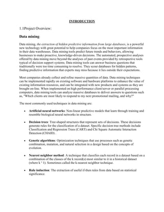
1.2. Software Process Model
Waterfall Model is one of the most widely used Software Development Process.It is also called as
"Linear Sequential model" or the "classic life cycle" or iterative model. It is widely used in the
commercial development projects. It is called so because here, we move to next phase(step) after
getting input from previous phase, like in a waterfall, water flows down to from the upper steps.

In this iterative waterfall model Software Development process is divided into five phases:-
a) SRS (Software Requirement Specifications)
b) System Design and Software Design
c) Implementation and Unit testing
d) Integration and System Testing
e) Operation and Maintenance

Iterative Waterfall Model with its stages

Lets discuss all these stages of waterfall model in detail.

Software Requirements Specifications:
This is the most crucial phase for the whole project, here project team along with the customer
makes a detailed list of user requirements. The project team chalks out the functionality and
limitations(if there are any) of the software they are developing, in detail. The document which
contains all this information is called SRS, and it clearly and unambiguously indicates the
requirements. A small amount of top-level analysis and design is also documented. This document is
verified and endorsed by the customer before starting the project. SRS serves as the input for further
phases.

System Design and Software Design:

Using SRS as input, system design is done. System design included designing of software and
hardware i.e. functionality of hardware and software is separated-out. After separation design of
software modules(see what is modularity) is done. The design process translates requirements into
representation of the software that can be assessed for quality before generation of code begins. At
the same time test plan is prepared, test plan describes the various tests which will be carried out on
the system after completion of development.

Implementation and Unit Testing:
Now that we have system design, code generation begins. Code generation is conversion of design
into machine-readable form. If designing of software and system is done well, code generation can be
done easily. Software modules are now further divided into units. A unit is a logically separable part
of the software. Testing of units can be done separately. In this phase unit testing is done by the
developer itself, to ensure that there are no defects.

Integration and System testing:
Now the units of the software are integrated together and a system is built. So we have a complete
software at hand which is tested to check if it meets the functional and performance requirements of
the customer. Testing is done, as per the steps defined in the test plan, to ensure defined input
produces actual results which agree with the required results. A test report is generated which
contains test results.

Operation & maintenance:
Now that we have completed the tested software, we deliver it to the client. His feed-backs are taken
and any changes, if required, are made in this phase. This phase goes on till the software is retired.

1.4 Roles and Responsibilities:

Everyone of the team members have done the job collaboratively. Everyone one of us have
done each and every job in a distributive manner. Each one of us shared the work and worked as
a team but not like an individual.

1.5 Tools and Techniques:
ABOUT ECLIPSE

Eclipse is a universal platform for integrating development tools Open, extensible
architecture based on plug-ins. Eclipse provides a number of aids that make writing Java code
much quicker and easier than using a text editor. This means that you can spend more time
learning Java, and less time typing and looking up documentation. The Eclipse debugger and

scrapbook allow you to look inside the execution of the Java code. This allows you to “see”
objects and to understand how Java is working behind the scenes. Eclipse provides full support
for agile software development practices such as test-driven development and refactoring.

Existing System

2.1Description of Existing System :

A mathematical algorithm for building the decision tree Invented by J. Ross Quinlan in
1939.Uses Information Theory invented by Shannon in 1941.Builds the tree from the top down,
with no backtracking. Employs a top-down greedy search through the space of possible decision
trees. Greedy because there is no backtracking. It picks highest values first. Information Gain is
used to select the most useful attribute for classification. Select attribute that is most useful for
classifying examples (attribute that has the highest Information Gain).

Iterative Dichotomiser 3 Algorithm is a Decision Tree learning algorithm. The name is correct in
that it creates Decision Trees for “dichotomizing” data instances, or classifying them discretely
through branching nodes until a classification “bucket” is reached (leaf node). By using ID3 and
other machine-learning algorithms from Artificial Intelligence, expert systems can engage in
tasks usually done by human experts, such as doctors diagnosing diseases by examining various
symptoms (the attributes) of patients (the data instances) in a complex Decision Tree. Accurate
Decision Trees are fundamental to Data Mining and Databases.

Decision tree learning is a method for approximating discrete-valued target functions, in which
the learned function is represented by a decision tree. Decision tree learning is one of the most
widely used and practical methods for inductive inference. The input data of ID3 is known as
sets of “training” or “learning” data instances, which will be used by the algorithm to generate
the Decision Tree. The machine is “learning” from this set of preliminary data.

The ID3 algorithm generates a Decision Tree by using a greedy search through the inputted sets
of data instances so as to determine nodes and the attributes they use for branching. Also, the
emerging tree is traversed in a top-down (root to leaf) approach through each of the nodes within
the tree. This occur RECURSIVELY, reminding you of those “pointless” tree traversals
strategies .The traversal attempts to determine if the decision “attribute” on which the branching
will be based on for any particular emerging node is the most ideal branching attribute by using

the inputted sets of data. One particular metric that can be used to determine then if a branching
attribute is adequate is that of INFORMATION GAIN, or ENTROPY.

ID3 uses Entropy to determine if, based on the inputted set of data, the selected branching
attribute for a particular node of the emerging tree is adequate. Specifically, the attribute that
results in the most reduction of Entropy related to the learning sets is the best.

GOAL: Find a way to optimally classify a learning set, such that the resulting Decision Tree is
not too deep and the number of branches (internal nodes) of the Tree is minimized.

SOLUTION: The more Entropy in a system or measure of impurity in a collection of data sets,
the m ore branches and depth the tree will have. FIND entropy reducing attributes in the
learning sets and use them for branching.

Information Gain = measuring the expected reduction in Entropy. The higher the Information
Gain, the more expected reduction in Entropy.

It turns out Entropy, or measure of non-homogeneousness within a set of learning sets can be
calculated in a straight forward manner.

CALCULATION AND CONSTRUCTION OF ID3 ALGORITHM

STEP1: Take the dataset and calculate the count of unique attribute values of the class label.

STEP2: Calculate amount of information for the class label by based on following formulae.

STEP3: Calculate the count of the each unique attribute values based on the unique attribute
values of the class label.

STEP4: Calculate expected information for each unique attribute value of each attribute by based
on following formulae.

STEP5: Calculate entropy value for each attribute. Here take the total expected information
values of all unique attribute values of the attribute at the time of calculation of entropy value by
based on following formulae.

STEP6: Calculate gain value with the help of amount of information value and entropy value by

STEP7: Construct the decision tree based on following decision tree algorithm.

EXPLANATION WITH EXAMPLE FOR ID3 DECISION TREE

Age, colour-cloth, income, student, buys _computer

>40, red, high, no, no

<30, yellow, high, no, no

30--40, blue, high, no, yes

>40, red, medium, no, yes

<30, white, low, yes, no

>40, red, low, yes, no

30--40, blue, low, yes, yes

<30, yellow, medium, no, yes

<30, yellow, low, yes, no

>40, white, medium, no, no

This one is the dataset of sample data set of buys computer

Attribute names: Age, colour-cloth, income, student, buys_computer

Unique values of attributes: >40, <30, 30—40, >40

Class labels of the dataset: yes, no

Step1:

For the given dataset first we have to calculate the information gain value for that we have to
know the count of class labels in the given dataset. That is NO’s count is 10 and YES’s count is
4. Then by using the formulae have to calculate the information gain value

No = 10 and yes=4

I (10, 4) =-10/4log2 (10/10)-4/10log2 (4/10)=0.4421+0.52107=0.9709

This calculating part is called amount of information and this is the unique value for the total
dataset.

Step2: calculate the each attributes with unique values, after that expected information and
entropy and gain values are calculated by formulae

Take the Age attribute and separate the values with comparison of class labels

No , yes count

>40  3 , 1 4

<30  3 , 1 4

30-40 - , 2 2

Total 10

This is the table for extracting data, based on the class labels of buys_ computer.

Now calculate the Expected Information for the unique attribute values of >40, <30, 30-40

>40 I(3,1)=-3/4log2 (3/4)-1/4log2 (1/4) = 0.10112

<30 I(3,1)=-3/4log2 (3/4)-1/4log2 (1/4) = 0.10112

30-40 I(0,2)= -2/2log2 (2/2)= 0

Now calculate the Entropy value for the Age attributes

E (age) =4/10(0.10112) +4/10(0.10112) +2/10(0)=0.324410+0.324410=0.10410910

Step3: calculate the Gain value for the age attribute based on amount of information and
entropy value

Gain (age) =I (s1, s2)-E (age) = 0.9709-0.10410910 = 0.32194

Second attribute: For color _cloth extracting the data based on the class labels of No, yes

No , yes count

Red  2 , 1 3

Yellow  2 , 1 3

Blue  - , 2 2

White  2 , - 2

Total 10

Calculate the Expected information for the color _ cloth

Red I (2, 1) =-2/3log2 (2/3)-1/3log2 (1/3) = 0.911029

Yellow I (2, 1) =-2/3log2 (2/3)-1/3log2 (1/3) = 0.911029

Blue I (0, 2) =-0/2log2 (0/2)-2/2log2 (2/2) = 0

White I (2, 0) =-2/2log2 (2/2) = 0

Now calculate the Entropy value for attribute color_cloth

E( color_cloth ) = 3/10(0.911029)+3/10(0.911029)+2/10(0)+2/10(0) = 0.550974

Gain value for color _ cloth

Gain (color_cloth) = I (s1, s2)-E (age) = 0.9709-0.550974= 0.41992

Third Attribute: For Income extracting the data based on the class labels of No, yes

No , yes count

High  1 , 2 3

Medium  2 , 1 3

Low  3 , 1 4

Total 10

Calculate the Expected information for the Income

High I (1, 2) =-1/3log2 (1/3)-2/3log2 (2/3) = 0.911029

Medium I (2, 1) =-2/3log2 (2/3)-1/3log2 (1/3) = 0.911029

Low I (3, 4) =-3/4log2 (3/4)-1/4log2 (1/4) = 0.10112

Now calculate the Entropy value for attribute Income

E( Income ) = 3/10(0.911029)+3/10(0.911029)+4/10(0.10112) = 0.1075454

Gain value for Income

Gain(income) = I (s1, s2)-E (Income) = 0.9709-0.1075454= 0.0954410

Fourth Attribute: For Student extracting the data based on the class labels of No, yes

No , yes count

No  3 , 3 6

Yes  1 , 3 4

Total 10

Calculate the Expected information for the student

No I (3,3) =-3/10log2 (3/10)-3/10log2 (3/10) = 1

Yes I (1,3) =-1/4log2 (1/4)-3/4log2 (3/4) = 0.10112

Now calculate the Entropy value for attribute student

E( Income ) = 10/10(1)+4/10(0.10112) = 0.924410

Gain value for student

Gain(student) = I (s1, s2)-E (Income) = 0.9709-0.924410= 0.041042

The important point is that , here compare the all Gain values what have calculated

Gain(age)=0.32194

Gain( color cloth )=0.41992highest Gain value

Gain(income)=0.954410

Gain(student)=0.041042

Color_cloth is the highest Gain value in the four attributes so that as per the algorithm it
becomes the Root Node while construction of the decision tree. After that take the unique
attribute values ( red , blue ,white, yellow) as the arcs and compare with the unique value red,
where we identify red attribute value in the dataset that all rows will be extract and form one
table that table called red attribute table like this we calculate the all Gain values after decide
where we have to place the right node , left node and leaf nodes.

In the above decision tree color_cloth is the root node remaining is attribute values of the
color_cloth. Based on the attribute values extract the data by neglecting the color_cloth attribute.
Here observe that first arc, we extract the data based on the red attribute value, where red
attribute is a look, take the total tuple values and calculate the expected information, entropy
value and at last gain value. This will be continued for left node, right node and leaf node
selections.

Red reference tuples

age,income,student,buys_computer

>40,high,no,no

>40,medium,no,yes

>40,low,yes,no

For Age extracting the data based on the class labels of No, yes

No , yes count

>40  2 , 1 3

Total 3


>40 I (2, 1) =-2/3log2 (2/3)-1/3log2 (1/3) = 0.911029


E( Income ) = 3/3(0.911029) = 0.911029

Gain value for Age

Gain(age) = I (s1, s2)-E (age) = 0.9709-0.911029= 0.0525

For Income extracting the data based on the class labels of No, yes

No , yes count

High  1 , 0 1

Medium  0 , 1 1

Low  1 , 0 1

Total 3


High I (1, 0) =-1/1log2 (1/1) = 0

Medium I (0, 1) =-1/1log2 (1/1) = 0

Low I (1, 0) =-1/1log2 (1/1) = 0


E( Income ) = 1/3(0)+1/3(0)+1/3(0) = 0


Gain(income) = I (s1, s2)-E (Income) = 0.9709-0= 0.9709

For Student extracting the data based on the class labels of No, yes

No , yes count

No  1 , 1 2

Yes  1 , 0 1

Total 3


No I (1,1) =-1/2log2 (1/2)-1/2log2 (1/2) = 1

Yes I (1,0) =-1/1log2 (1/1) = 0


E( Income ) = 2/3(1)+1/3(0) = 0.1010107


Gain(student) = I (s1, s2)-E (student) = 0.9709-0.1010107= 0.3043

Here again calculate the expected information,entropy and gain values of Red table.

Gain values of age , income , student are 0.05210 , 0.9709 , 0.3043

Here income have the highest gain value so left node is income.

Blue reference tuples


30-40, high, no, yes

30-40, low, yes, yes


No , yes count

30-40  0 , 2 2

Total 2


30-40 I (0, 2) =-2/2log2 (2/2) = 0

Now calculate the Entropy value for attribute age

E( age ) = 2/2(0) = 0

Gain value for Age

Gain(age) = I (s1, s2)-E (age) = 0.9709-0= 0


No , yes count

High  0 , 1 1

Low  0 , 1 1

Total 2


High I (0, 1) =-1/1log2 (1/1) = 0

Low I (0, 1) =-1/1log2 (1/1) = 0


E( Income ) = 1/2(0)+1/2(0) = 0




No , yes count

No  0 , 1 1

Yes  0 , 1 1

Total 2


No I (0,1) =-1/1log2 (1/1) = 0

Yes I (0,1) =-1/1log2 (1/1) = 0


E( Income ) = 1/2(0)+1/2(0) = 0


Gain(student) = I (s1, s2)-E (student) = 0.9709-0= 0.9709

Gain values of age, income, and student are 0.9709, 0.9709, 0.9709

Here all the values are same so node is ended here.

White reference tuples


<30, low, yes, no

>40, medium, no, no


No , yes count

<30  1 , 0 1

>40  1 , 0 1

Total 2


<30 I (1, 0) =-2/2log2 (2/2) = 0

>40 I (1, 0) =-2/2log2 (2/2) = 0

Now calculate the Entropy value for attribute age

E( age ) = 1/2(0)+1/2(0) = 0

Gain value for Age

Gain(age) = I (s1, s2)-E (age) = 0.9709-0= 0


No , yes count

Low  1 , 0 1

Medium  1 , 0 1

Total 2


Medium I (1, 0) =-1/1log2 (1/1) = 0

Low I (1, 0) =-1/1log2 (1/1) = 0


E( Income ) = 1/2(0)+1/2(0) = 0




No , yes count

No  1 , 0 1

Yes  1 , 0 1

Total 2


No I (1,0) =-1/1log2 (1/1) = 0

Yes I (1,0) =-1/1log2 (1/1) = 0


E( Income ) = 1/2(0)+1/2(0) = 0



Gain values of age, income, and student are 0.9709, 0.9709, and 0.9709

Here all the values are same so node is ended here.

Yellow reference tuples


<30, high, no, no

<30, medium, no, yes

<30, low, yes, no


No , yes count

<30  2 , 1 3

Total 3


>40 I (2, 1) =-2/3log2 (2/3)-1/3log2 (1/3) = 0.911029


E( Income ) = 3/3(0.911029) = 0.911029

Gain value for Age

Gain(age) = I (s1, s2)-E (age) = 0.9709-0.911029= 0.0525


No , yes count

High  1 , 0 1

Medium  0 , 1 1

Low  1 , 0 1

Total 3


High I (1, 0) =-1/1log2 (1/1) = 0

Medium I (0, 1) =-1/1log2 (1/1) = 0

Low I (1, 0) =-1/1log2 (1/1) = 0


E( Income ) = 1/3(0)+1/3(0)+1/3(0) = 0




No , yes count

No  1 , 1 2

Yes  1 , 0 1

Total 3


No I (1,1) =-1/2log2 (1/2)-1/2log2 (1/2) = 1

Yes I (1,0) =-1/1log2 (1/1) = 0


E( Income ) = 2/3(1)+1/3(0) = 0.1010107



Gain values of age , income , student are 0.052101, 0.9709, 0.3043

Here income gain value is high so right node is constructed.

CONSTRUCTION OF ID3 DECISION TREE ALGORITHM

STEP1: Calculate gains of the Attributes.

STEP2: Make one attribute as a Root Node which has the highest gain.

STEP3: Calculate datasets based on the current node unique attribute values by neglecting the
current node attribute values dataset and current node is the parent node.

STEP4: Take each dataset from the datasets and go to step5.

STEP5: Take current one as attributes. If attribute values size is one then go to step6 else go to
step7

STEP6: Consider the current one as a leaf node to the parent node.

STEP7: Calculate Attribute Gains

STEP8: If all Attribute Gains are same then go to step6 else make one attribute as a Node which
has the highest gain and consider this node as a current node and go to step3.

2.2 Flaws or Drawbacks with Existing System:

The principle of selecting attribute A as test attribute for ID3 is to make E (A) of attribute A, the
smallest. Study suggest that there exists a problem with this method, this means that it often
biased to select attributes with more taken values however, which are not necessarily the best

attributes. In other words, it is not so important in real situation for those attributes selected by
ID3 algorithm to be judged firstly according to make value of entropy minimal. Besides, ID3
algorithm selects attributes in terms of information entropy which is computed based on
probabilities, while probability method is only suitable for solving stochastic problems. Aiming
at these shortcomings for ID3 algorithm, some improvements on ID3 algorithm are made and a
improved decision tree algorithm is introduced.

3. Proposed System

3.1Description of Proposed System:

The principle of selecting attribute A as test attribute for ID3 is to make E (A) of
attribute A, the smallest. Study suggest that there exists a problem with this method, this means
that it often biased to select attributes with more taken values however, which are not necessarily
the best attributes. In other words, it is not so important in real situation for those attributes
selected by ID3 algorithm to be judged firstly according to make value of entropy minimal.
Besides, ID3 algorithm selects attributes in terms of information entropy which is computed
based on probabilities, while probability method is only suitable for solving stochastic problems.
Aiming at these shortcomings for ID3 algorithm, some improvements on ID3 algorithm are made
and a improved decision tree algorithm is introduced.

3.2Problem Statement:
Decision tree is an important method for both induction research and data mining, which is
mainly used for model classification and prediction. ID3 algorithm is the most widely used
algorithm in the decision tree. Through illustrating on the basic ideas of decision tree in data
mining, in my paper, the shortcoming of ID3’s inclining to choose attributes with many values,
however, which are not necessarily the best attributes. In other words, it is not so important in
real situation for those attributes selected by ID3 algorithm to be judged firstly according to
make value of entropy minimal. Besides, ID3 algorithm selects attributes in terms of information
entropy which is computed based on probabilities, while probability method is only suitable for
solving stochastic problems. Aiming at these shortcomings for ID3 algorithm, a new decision

tree algorithm combining ID3 and Association Function is presented. The experiment results
show that the proposed algorithm can overcome ID3’s shortcoming effectively and get more
reasonable and effective rules.

3.3 Working of Proposed System:

CALCULATION OF IMPROVED ID3 ALGORITHM

STEP1: Take the dataset and calculate the count of unique attribute values of the class label.

STEP2: Calculate amount of information for the class label by based on following formulae.

STEP3: Calculate the count of the each unique attribute values based on the unique attribute
values of the class label.

STEP4: Calculate expected information for each unique attribute value of each attribute by

STEP5: Calculate entropy value for each attribute. Here take the total calculated expected
information values of all unique attribute values of entropy value by based on following
formulae.

STEP6: Calculate gain value with the help of amount of information value and entropy value by

STEP7: After calculating gain values here again we calculate the importance of attribute by
using correlation function method for each attribute by based on following formulas. Here a
formula gives for only two cases class labels. While in two conditions only this formulae works

STEP8: Calculate the Improved ID3 gain of each attribute with the help of ID3, amount of
information and correlation function by using following formulae.

xV (k)

Till now the calculation part is as same as id3 algorithm, In improved id3 algorithm has to
calculate the importance of the each attribute after that multiply the correlation factor with the
id3 gain values that calculation is as follows by using datasets of the id3 that attribute values
have to calculate the ASSOCIATION FUNCTION expansion as below

AF (A) = this formula is applied on retrieved datasets.

Example takes the all attribute values from age, color_cloth, income, and student

Age data

No , yes count

>40  3 , 1 4

<30  3 , 1 4

30-40 - , 2 2

Total 10

Calculation for all datasets

AF (age) = =2

AF (color_cloth) = =1.5

AF (income) = =1.3334

AF (student) = =1

THE NORMALIZATION RELATION DEGREE FORMULA

=0.34210

=0.2571

=0.22105

NOW CALCULATE THE IMPROVED ID3 GAIN VALUE BY USING THE FORMULA

xV (K)

Gain (age) = 0.32194 x 0.34210= 0.110310 highest gain value in improved id3 decision tree so it is the root node

Gain (color_cloth) = 0.41992 x 0.2571= 0.107910

Gain (income) = 0.0954410 x 0.22105= 0.021100

Gain (student) = 0.041042 x 0.1714= 0.0079510

So AGE attribute becomes root node. <30, 30-40 and >40 are the unique attribute values.

Now extract the <30,30-40,>40 data from dataset.

Color_cloth, income, student, buys_computer here we neglect the age attribute because of, it was
the root node. so take the references of age attribute values and retrieve the total <30 tuple
values.

<30 dataset

Color_cloth, income, student, buys_computer

Yellow, high, no, no

White, low, yes, no

Yellow, medium, no, yes

Yellow, low, yes, no

Here calculate the gain values for color-cloth

No , yes count

Yellow  2 , 1 3

White  1 , - 1

Total 4

For color-cloth extracting the data based on the class labels of No, yes

No , yes count

yellow  2 , 1 3

white  1 , 0 1

Total 4

Calculate the Expected information for the color-cloth

yellow I (2, 1) =-2/3log2 (2/3)-1/3log2 (1/3) = 0.911029

white I(1,0)=-1/1log(1/1)=0


E( color-cloth) = 3/4(0.911029) +1/4(0)= 0.10101010

Gain value for color-cloth

Gain(color-cloth) = I (s1, s2)-E (color-cloth) = 0.9709-0.10101010= 0.21022


No , yes count

High  1 , 0 1

Medium  0 , 1 1

Low  2 , 0 2

Total 4


High I (1, 0) =-1/1log2 (1/1) = 0

Medium I (0, 1) =-1/1log2 (1/1) = 0

Low I (2, 0) =-2/2log2 (2/2) = 0


E( Income ) = 1/4(0)+1/4(0)+1/4(0) = 0




No , yes count

No  1 , 1 2

Yes  2 , 0 2

Total 4


No I (1,1) =-1/2log2 (1/2)-1/2log2 (1/2) = 1

Yes I (2,0) =-2/2log2 (2/2) = 0


E( Income ) = 2/4(1)+2/4(0) = 0.5



AF (color_cloth) = =1

AF (income) = =1.3334

AF (student) = =1

=0.2999

=0.4

Gain values are


Gain (income) = 0.9709 x 0.4= 0.310103

Gain (student) = 0.47010 x 0.2999= 0.1411

Income has the highest gain value

30 - 40 dataset


Blue , high, no, yes

Blue , low, yes, yes

Here calculate the gain values for color-cloth

No , yes count

Blue  0 , 2 2

Total 2


Blue I(0,2)=-2/2log(2/2)=0


E( color-cloth ) = 2/2(0)= 0


Gain(color-cloth) = I (s1, s2)-E (color-cloth) = 0.9709-0= 0.9709


No , yes count

High  0 , 1 1

Low  0 , 1 1

Total 2


High I (1, 0) =-1/1log2 (1/1) = 0

Low I (1, 0) =-1/1log2 (1/1) = 0


E( Income ) = 1/2(0)+1/2(0) = 0




No , yes count

No  0 , 1 1

Yes  0 , 1 1

Total 2


No I (0,1) =-1/1log2 (1/1) = 0

Yes I (0,1) =-1/1log2 (1/1) = 0


E( Income ) = 1/2(0)+1/2(0) = 0




AF (income) = =1

AF (student) = =1

=0.5

=0.25

Gain values are


Gain (income) = 0.9709 x 0.25= 0.2427

Gain (student) = 0.9709 x 0.25= 0.2427

Color-cloth has the highest gain value

>40 dataset


Red , high, no, no

Red , low, yes, no

Red , medium, no, yes

White , medium, no, no


No , yes count

white  1 , 0 1

red  2 , 1 3

Total 4


Red I (2, 1) =-2/3log2 (2/3)-1/3log2 (1/3) = 0.911029

white I(1,0)=-1/1log(1/1)=0


E( color-cloth) = 3/4(0.911029) +1/4(0)= 0.10101010


Gain(color-cloth) = I (s1, s2)-E (color-cloth) = 0.9709-0.10101010= 0.21022


No , yes count

High  1 , 0 1

Medium  1 , 1 2

Low  1 , 0 1

Total 4


High I (1, 0) =-1/1log2 (1/1) = 0

Medium I (1, 1) =-1/2log2 (1/1)-1/2log(1/2) = 1

Low I (1, 0) =-1/1log2 (1/1) = 0


E( Income ) = 1/4(0)+2/4(1)+1/4(0) = 0.5


Gain(income) = I (s1, s2)-E (Income) = 0.9709-0.5= 0.4709


No , yes count

No  2 , 1 3

Yes  1 , 0 1

Total 4


No I (2,1) =-2/3log2 (2/3)-1/3log2 (1/3) = 0.9110295

Yes I (1,0) =-1/1log2 (1/1) = 0


E( Income ) = 3/4(0.9110295)+1/4(0) = 0.1010107




AF (income) = =0.1010107

AF (student) = =1

=0.3749

=0.25

Gain values are


Gain (income) = 0.4709 x 0.25= 0.1177

Gain (student) = 0.21022 x 0.3749= 0.1057

Income has the highest gain value

>40 Income dataset for high

Color-cloth, student, buys-computer

Red, no, no

Class lable is same for both color-cloth and student, hence it becomes leaf node.

>40 Income dataset for low


Red, yes , no


>40 Income dataset for medium


Red, no , yes

White, no, no


No , yes count

white  1 , 0 1

red  0 , 1 1

Total 2


Red I (0, 1) =-1/1log2 (1/1)=0

white I(1,0)=-1/1log(1/1)=0


E( color-cloth) = 1/2(0) +1/2(0)= 0


Gain(color-cloth) = I (s1, s2)-E (color-cloth) = 0.9709-0= 0.9709


No , yes count

No  1 , 1 2

Total 2


No I (1,1) =-1/2log2 (1/2)-1/2log2 (1/2) = 1


E( Income ) = 2/2(1) = 1


Gain(student) = I (s1, s2)-E (student) = 0.9709-1= -0.0292


AF (student) = =0

=1

Gain values are

Gain (color_cloth) = 0.9709 x 1= 0.9709

Gain (student) = -0.0292 x 0= 0

<30 Income dataset for high


Yellow , no , no


<30 Income dataset for low


White , yes , no

Yellow, yes, no


<30 Income dataset for medium


Yellow , no , yes


Construction of Improved ID3 decision tree:

4. Requirement Analysis or Requirements Elicitation
REQUIREMENT SPECIFICATION:

A requirement is a feature that the system must have or a constraint that it must satisfy to
be accepted by the client. Requirement engineering aims at defining the requirements of the
system under construction. Requirement engineering include two main activities, requirements
elicitation, which results in the specification of the system that the client understands, and
analysis, which results in an analysis model that the developer can unambiguously interpret. A
requirement is statement about what the proposed system will do. Requirements can be divided
into two major categories: functional requirements and non- functional requirements.

4.1 Functional requirements:

Functional requirements describe the interactions between the system and its
environment independent of its implementation. The environment includes the user and any
other external system with which the system interacts.

4.2 Non Functional Requirements:

Non-functional requirements describe aspects of the system that are not directly related
the functional behaviour of the system. Non-functional requirements include a broad variety of
requirements that apply to many different aspects of the system, from usability to performance.

4.2.1 Software Requirements:

Operating System : Windows 2000/XP IDE

Language : JDK 1.5

Eclipse Documentation : MS-Word

Designing : Rational rose

4.2.2 Hardware Requirements:

CPU : Pentium IV

RAM : 512MB.

Hard Disk : 40GB.

Input device : Standard Keyboard and Mouse.
Output device : VGA and High Resolution Monitor

Introduction

Recommended

Recommended

More Related Content

What's hot

What's hot (20)

Viewers also liked

Viewers also liked (20)

Similar to Introduction

Similar to Introduction (20)

Introduction