Detaled working and calculation of integral method to solve kinetcs problem

1. THE INTEGRAL AND THE DIFFERENTIAL METHODS
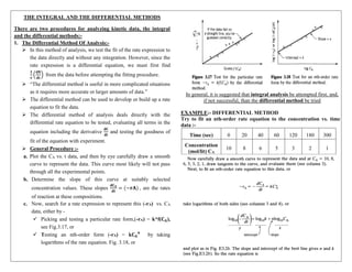
There are two procedures for analyzing kinetic data, the integral
and the differential methods:-
1. The Differential Method Of Analysis:-
➢ In this method of analysis, we test the fit of the rate expression to
the data directly and without any integration. However, since the
rate expression is a differential equation, we must first find
𝟏
𝐯
(
𝐝𝐍
𝐝𝐭
) from the data before attempting the fitting procedure.
➢ “The differential method is useful in more complicated situations
as it requires more accurate or larger amounts of data.”
➢ The differential method can be used to develop or build up a rate
equation to fit the data.
➢ The differential method of analysis deals directly with the
differential rate equation to be tested, evaluating all terms in the
equation including the derivative
𝐝𝐂
𝐝𝐭
and testing the goodness of
fit of the equation with experiment.
➢ General Procedure :-
a. Plot the CA vs. t data, and then by eye carefully draw a smooth
curve to represent the data. This curve most likely will not pass
through all the experimental points.
b. Determine the slope of this curve at suitably selected
concentration values. These slopes
𝐝𝐂𝐀
𝐝𝐭
= (−𝐫𝐀) , are the rates
of reaction at these compositions.
c. Now, search for a rate expression to represent this (-rA) vs. CA
data, either by -
✓ Picking and testing a particular rate form,(-rA) = k*f(𝐂𝐀),
see Fig.3.17, or
✓ Testing an nth-order form (-rA) = k𝐂𝐀
𝐧
by taking
logarithms of the rate equation. Fig. 3.18, or
In general, it is suggested that integral analysis be attempted first, and,
if not successful, than the differential method be tried
EXAMPLE:- DIFFERENTIAL METHOD
Try to fit an nth-order rate equation to the concentration vs. time
data :-
Time (sec) 0 20 40 60 120 180 300
Concentration
(mol/lit) CA
10 8 6 5 3 2 1

2. 2. The Integral Method Of Analysis :-
➢ In this method of analysis, we guess a particular form of rate
equation and, after appropriate integration and mathematical
manipulation, predict that the plot of a certain concentration
function versus time should yield a straight line. The data are
plotted, and if a reasonably good straight line is obtained, then
the rate equation is said to satisfactorily fit the data.
➢ “The integral method is easy to use and is recommended when
testing specific mechanisms, or relatively simple rate
expressions, or when the data are so scattered that we cannot
reliably find the derivatives needed in the differential method.”
➢ The integral method can only test this or that particular
mechanism or rate form.
➢ General Procedure :-
a) The integral method of analysis always puts a particular
rate equation to the test by integrating and comparing the
predicted C versus t curve with the experimental C versus
t data.
b) If the fit is unsatisfactory, another rate equation is guessed
and tested.
c) This procedure is shown and used in the cases next
treated. It should be noted that the integral method is
especially useful for fitting simple reaction types
corresponding to elementary reactions.
1, - 0.875
0, - 2.305

3. Let us consider the following example:-
A plot of In (1 - XA) or In (CA/CAo) v/s t, as shown in Fig. 3.1, gives a
straight line through the origin for this form of rate of equation.
If the experimental data seems to be better fitted by a
curve than by a straight line, try another rate form because
the first-order reaction does not satisfactorily fit the data.
Example 1 :- INTEGRAL METHOD
The composition of A in the reactor is measured at various times
with results shown in the following columns 1 and 2. Find a rate
equation to represent the data.

4. Case 1 : - Assume the reaction is first order -→
Start by guessing the simplest rate form, or first order kinetics. This
means that In (CAo/CA) v/s t, should give a straight line, see Eq. 11
or 12, or Fig. 3.1.
So, column 3 is calculated and the plot of Fig. E3.la is made.
.
 Unfortunately, this does not give a straight line, so first-
order kinetics cannot reasonably represent the data, and
we must guess another rate form
Case 2 : - Assume the reaction is Second order -→
Equation 16 tells that 1/C vs. t should give a straight line. So,
calculate column 4, plot column 1 vs, column 4, as shown in Fig.
E3.lb.

5. Again, this does not give a straight line, so a second-order kinetic
form is rejected.
We now have the reaction order using slope from above line.
𝐒𝐋𝐎𝐏𝐄 =
(𝟏. 𝟐𝟕 − 𝟏. 𝟓𝟒)
(𝟏 − 𝟎. 𝟑)
 -0.3857
 -0.04 (Approximately)
Hence, 𝑺𝒍𝒐𝒑𝒆 = 𝟏 − 𝒏 = −𝟎. 𝟒
 n = 1 - (-0.4)
 n = 1.4

6. To evaluate the rate constant, take any point on the CA vs. t
curve. Pick CAo = 10, for which tf = 18.5 s.
Replacing all values into Eq. (i) gives -
2. Rearranging above, we get –
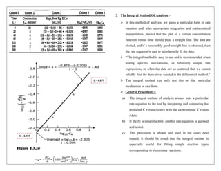
 𝐥𝐧([𝐀]𝟏𝐭)/𝟎. 𝟐) = −𝐊𝟏𝐭 (Straight line eqn : - y = mx + c)
Time (min) [A]1t (mol/L)
 ln([A]1t)/[A10])
Or
 ln([A]1t)/0.2)
0 0.2 0
10 0.15 -0.124938737
20 0.1 -0.301029996
30 0.07 -0.455931956
40 0.05 -0.602059991
DATA TABLE ASSUMING REACTION 1 IS A FIRST ORDER
REACTION
18.5, 8

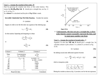
7. Analysis for Reaction 1:
The plot shows a clear linear relationship, confirming first-order
kinetics. Therefore, the rate expression for Reaction 1 is:
But, the value of K1 will be –
𝐾1 = (− 𝑆𝑙𝑜𝑝𝑒)
(𝐅𝐨𝐫 𝐞𝐪𝐮𝐚𝐭𝐢𝐨𝐧 𝐨𝐟 𝐬𝐭𝐫𝐚𝐢𝐠𝐡𝐭 𝐥𝐢𝐧𝐞 𝐰𝐢𝐭𝐡 𝟐 𝐩𝐨𝐧𝐭 𝐤𝐧𝐨𝐰𝐧) −
 𝐬𝐥𝐨𝐩𝐞 = [
(𝐲𝟐−𝐲𝟏)
(𝐱𝟐−𝐱𝟏)
]
 [
(−𝟎.𝟔−𝟎)
(𝟒𝟎−𝟎)
] = -0.015
Hence, the value of K1 will be –
𝐾1 = (− 𝑆𝑙𝑜𝑝𝑒) = −(−0.015)
 0.015
Therefore, the rate expression for Reaction 1 is:
(−𝐫𝐀) = 𝟎. 𝟎𝟏𝟓 𝐂𝐀
𝟏
ln([A]1t)/0.2)
 ln([A]1t)/0.2)