1. rsnSieve: a matlab application for automatic
resting state network selection using ICA
Tyler L. Coyea
aDepartment of Neurology, The University of Pennsylvania
1. Introduction
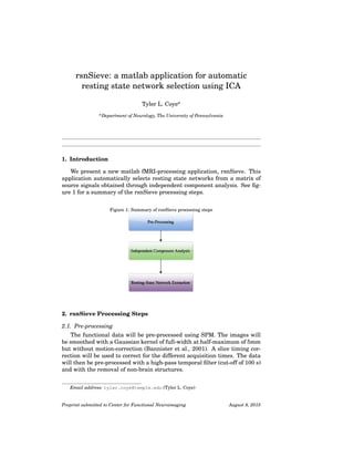
We present a new matlab fMRI-processing application, rsnSieve. This
application automatically selects resting state networks from a matrix of
source signals obtained through independent component analysis. See fig-
ure 1 for a summary of the rsnSieve processing steps.
Figure 1: Summary of rsnSieve processing steps
2. rsnSieve Processing Steps
2.1. Pre-processing
The functional data will be pre-processed using SPM. The images will
be smoothed with a Gaussian kernel of full-width at half-maximum of 5mm
but without motion-correction (Bannister et al., 2001). A slice timing cor-
rection will be used to correct for the different acquisition times. The data
will then be pre-processed with a high-pass temporal filter (cut-off of 100 s)
and with the removal of non-brain structures.
Email address: tyler.coye@temple.edu (Tyler L. Coye)
Preprint submitted to Center for Functional Neuroimaging August 8, 2015

2. 2.2 Spatial ICA 2
Figure 2: Spatial ICA of fMRI
image was obtained from http://users.ics.aalto.fi/whyj/publications/thesis/thesis_node8.html
2.2. Spatial ICA
The model used in ICA is a statistical generative model for an instan-
taneous linear mixture of random variables. When the mixed signals are
represented as a data matrix X, the mixing model can be expressed in the
matrix form as:
X = AS (1)
Each row of the source matrix S contains one independent component
and each column of the mixing matrix A holds the corresponding weights,
for a total of K sources.
To be able to use the fMRI signal in the ICA model, each scanned vol-
ume must be transformed into vector form in a bidirectional manner. The
fMRI signal is represented by a TxV data matrix X , where T is the number
of time points and V is the number of voxels in the volumes. This means
that each row of S contains an independent spatial pattern and the corre-
sponding column of A holds its activation time-courses. See figure 2 for an
illustration of this model.
The fastICA algorithm (FastICA, 1998, Hyvärinen, 1999) uses a fixed-
point optimization scheme based on Newton-iteration and an objective func-
tion related to negentropy. The idea is to first whiten the data using PCA
and then, based on the whitened data matrix X, search for a solution in
the form s = wT
x, where s and x are columns of the source matrix and
whitened data matrix, respectively. Or equivalently in matrix form:
S = WX, (2)
where W = AT
is the demixing matrix. The algorithm optimizes the ob-
jective function, which estimates the sources S by approximating statistical
independence. The algorithm starts from an initial condition, for example,
random mixing weights w . Then, on each iteration step, the weights w
are first updated, so that the corresponding sources become more indepen-
dent, and then normalized, so that W stays orthonormal. The iteration is
continued until the weights converge.

3. 2.3 Automatic selection of resting state networks 3
2.3. Automatic selection of resting state networks
We start with the K sources in S as estimated by fastICA. We are go-
ing to filter these components to select the optimal number of components
related to resting state networks. Our extraction process is based on a mod-
ified approach first discussed by Storti et al. (2013). Our approach will be
unique in that it is applied only to single subjects. See figure 3 for an outline
of the steps we will take to extract the resting state network components.
Figure 3: summary of resting-state network extraction
2.3.1. Pearson’s index evaluation (PIE)
Each independent component is in a row of matrix S. We want to de-
termine whether the data is symmetric or skewed. To do this, we look at
Pearson’s index of skewness of each row in S. Pearson’s second skewness
coefficient is defined as:
PC = 3
mean − median
σ
, (3)
where σ is the standard deviation. Noise components will have a PC
close to 0. We reject the independent components if the PC of the elements
in the corresponding row of S is lower than a selected threshold (TH). The
selected threshold is the median of the Pearson’s indexes of all elements in
S. Rejected independent components are moved to the last position and set
to 0. After this step, S will have non-zero rows less than or equal to K.
2.3.2. Silhouette k-means clustering
In this step we will apply cluster analysis using a k-means algorithm
(MacQueen, 1967; Golay et al., 1998; Goutte et al., 1999). This will remove
voxels associated with low values for each component. Clustering is ap-
plied to each non-zero row of S. We perform this analysis to separate the
candidate of each non-zero row in S in K clusters. This step will set to zero
some voxel elements in the columns of S. After clustering, we will eliminate

4. 2.3 Automatic selection of resting state networks 4
voxels belonging to the cluster with the centroid nearest 0. This cluster con-
tains voxels with the lowest activation values. We will use the silhouette
value (Kaufman and Rousseeuw, 1990) to optimize clustering quality.
Assuming a specific row of S, the optimal number of clusters to be used
for the values of this selected row was determined by using the method
proposed in Zhang et al. (2011) based on the evaluation of the silhouette
index. The silhouette value for each point is a measure of how similar
that point is to points in its own cluster, when compared to points in other
clusters. The silhouette value for point i in S , SVi, is defined as
SVi =
(bi − ai)
max(bi, ai)
(4)
where ai is the average distance from point i to the other points in the
same cluster as i, and bi is the minimum average distance from point i
to points in a different cluster, minimized over clusters. The silhouette
value ranges from -1 to +1. A high silhouette value indicates that i is well-
matched to its own cluster, and poorly-matched to neighboring clusters. If
most points have a high silhouette value, then the clustering solution is
appropriate. We will determine the number of clusters by maximizing the
average silhouette value.
2.3.3. Segmentation
After fastICA decomposition, the S matrix will include signals from sub-
cortical structures such as white matter and ventricals. To restrict activa-
tion to the gray matter, the fMRI data will be segmented with SPM. The
voxels in each component with at least 90% probability of belonging to the
white matter or CSF will be cancelled (Keihaninejad et al., 2010; Polanía
et al., 2012).
2.3.4. Relative power spectral analysis
For each component identified above, the relative fMRI time courses will
be baseline corrected, detrended and averaged. For each component, the
mean fMRI time series will then be transformed to a frequency domain with
the fast Fourier transform (using the periodogram method). The relative
power of each component in select frequency bands will be obtained. We
will estimate the relative power in three bands: P1[0 − 0.01Hz], P2[0.01 −
0.1Hz], and P3[> 0.1Hz]. If a signal x(t) has Fourier transform X(f), its
power spectral density is |X(f)|2
= SX(f). The absolute spectral power
in the band of frequencies f0Hz to f1Hz is the total power in that band
of frequencies, that is, the total power delivered at the output of an ideal
(unit gain) band pass filter that passes all frequencies from f0Hz to f1Hz
hertz and stop everything else. Thus, the Absolute Spectral Power in Band
(SPBabs) is:
ASPB =
ˆ −f0
−f1
Sx(f)df +
ˆ f1
f0
Sx(f)df. (5)

5. 5
The relative spectral power measures the ration of the total power in the
band (i.e., absolute spectral power) to the total power in the signal. Thus,
the Relative Spectral Power Band (RSPB) is:
RSPD =
´ −f0
−f1
Sx(f)df +
´ f1
f0
Sx(f)df
´ ∞
−∞
Sx(f)df
. (6)
Using (5) and (6) we write for P1, P2, and P3:
P1 =
´ .01
0
Sx(f)
´ b
0
Sx(f)
df, (7)
P2 =
´ .1
.01
Sx(f)
´ b
0
Sx(f)
df, (8)
P3 =
´ b
.1
Sx(f)
´ b
0
Sx(f)
df, (9)
where b depends on the acquisition parameters. RSNs are characterized
by slow fluctuations of functional imaging signals between 0.01 and 0.1 Hz
(P2) (Cordes et al., 2000; Damoiseaux et al., 2006; De Martino et al., 2007;
Mantini et al., 2007). Therefore, the components with P2 < 50% and with
P1 + P2 < 90% will be rejected. We will also filter out components with
P2 > 50% since intrinsic connectivity is detected in the very low-frequency
ranges (Cordes et al., 2001).
3. References
[1] Bannister, P. R., Beckmann, C., & Jenkinson, M. (2001). Exploratory
motion analysis in fMRI using ICA. NeuroImage, 6(13), 69.
[2] Cordes, D., Haughton, V. M., Arfanakis, K., Wendt, G. J., Turski, P.
A., Moritz, C. H., ... & Meyerand, M. E. (2000). Mapping function-
ally related regions of brain with functional connectivity MR imaging.
American Journal of Neuroradiology, 21(9), 1636-1644.
[3] Cordes, D., Haughton, V. M., Arfanakis, K., Carew, J. D., Turski, P. A.,
Moritz, C. H., ... & Meyerand, M. E. (2001). Frequencies contributing
to functional connectivity in the cerebral cortex in “resting-state” data.
American Journal of Neuroradiology, 22(7), 1326-1333.aut
[4] Damoiseaux, J. S., Rombouts, S. A. R. B., Barkhof, F., Scheltens,
P., Stam, C. J., Smith, S. M., & Beckmann, C. F. (2006). Consistent
resting-state networks across healthy subjects. Proceedings of the na-
tional academy of sciences, 103(37), 13848-13853.

6. 6
[5] De Martino, F., Gentile, F., Esposito, F., Balsi, M., Di Salle, F., Goebel,
R., & Formisano, E. (2007). Classification of fMRI independent com-
ponents using IC-fingerprints and support vector machine classifiers.
Neuroimage, 34(1), 177-194.
[6] Golay, X., Kollias, S., Stoll, G., Meier, D., Valavanis, A., & Boesiger,
P. (1998). A new correlation-based fuzzy logic clustering algorithm for
FMRI. Magnetic Resonance in Medicine, 40(2), 249-260.
[7] Goutte, C., Toft, P., Rostrup, E., Nielsen, F. Å., & Hansen, L. K. (1999).
On clustering fMRI time series. NeuroImage, 9(3), 298-310.
[8] Hyvärinen, A., & Oja, E. (1998). The Fast-ICA MATLAB package.
[9] Hyvärinen, A. (1999). Fast and robust fixed-point algorithms for in-
dependent component analysis. Neural Networks, IEEE Transactions
on, 10(3), 626-634.
[10] Kaufman, L., & Rousseeuw, P. J. (2009). Finding groups in data: an
introduction to cluster analysis (Vol. 344). John Wiley & Sons.
[11] Keihaninejad, S., Heckemann, R. A., Fagiolo, G., Symms, M. R., Ha-
jnal, J. V., Hammers, A., & Alzheimer’s Disease Neuroimaging Ini-
tiative. (2010). A robust method to estimate the intracranial volume
across MRI field strengths (1.5 T and 3T). Neuroimage, 50(4), 1427-
1437.
[12] MacQueen, J. (1967, June). Some methods for classification and anal-
ysis of multivariate observations. In Proceedings of the fifth Berkeley
symposium on mathematical statistics and probability (Vol. 1, No. 14,
pp. 281-297).
[13] Mantini, D., Perrucci, M. G., Del Gratta, C., Romani, G. L., & Corbetta,
M. (2007). Electrophysiological signatures of resting state networks in
the human brain. Proceedings of the National Academy of Sciences,
104(32), 13170-13175.
[14] Polanía, R., Paulus, W., & Nitsche, M. A. (2012). Reorganizing the in-
trinsic functional architecture of the human primary motor cortex dur-
ing rest with non-invasive cortical stimulation. PloS one, 7(1), e30971.
[15] Storti, S. F., Formaggio, E., Nordio, R., Manganotti, P., Fiaschi, A.,
Bertoldo, A., & Toffolo, G. M. (2013). Automatic selection of resting-
state networks with functional magnetic resonance imaging. Frontiers
in neuroscience, 7.
[16] Zhang, J., Tuo, X., Yuan, Z., Liao, W., & Chen, H. (2011). Analysis
of FMRI data using an integrated principal component analysis and
supervised affinity propagation clustering approach. Biomedical Engi-
neering, IEEE Transactions on, 58(11), 3184-3196.