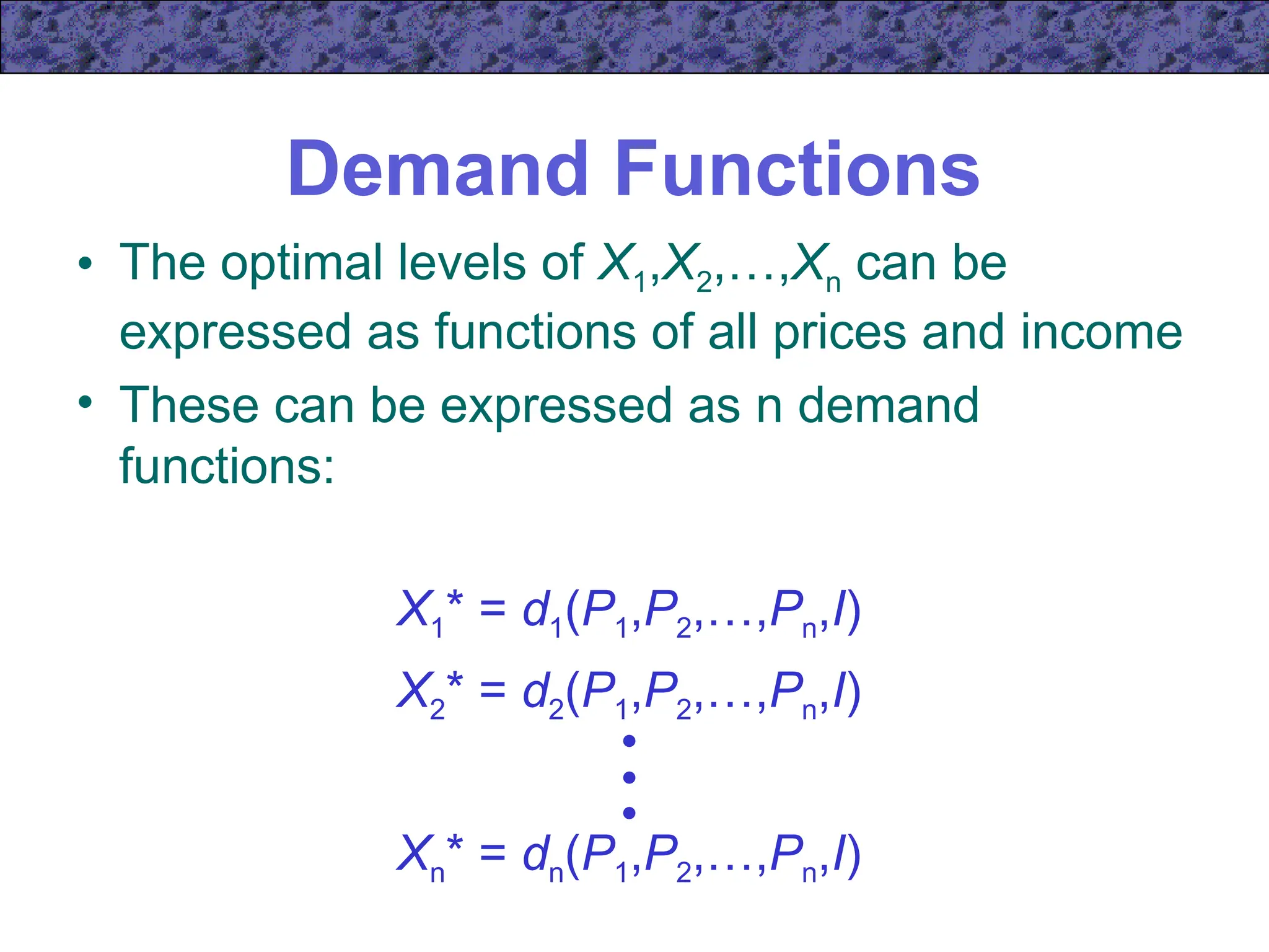
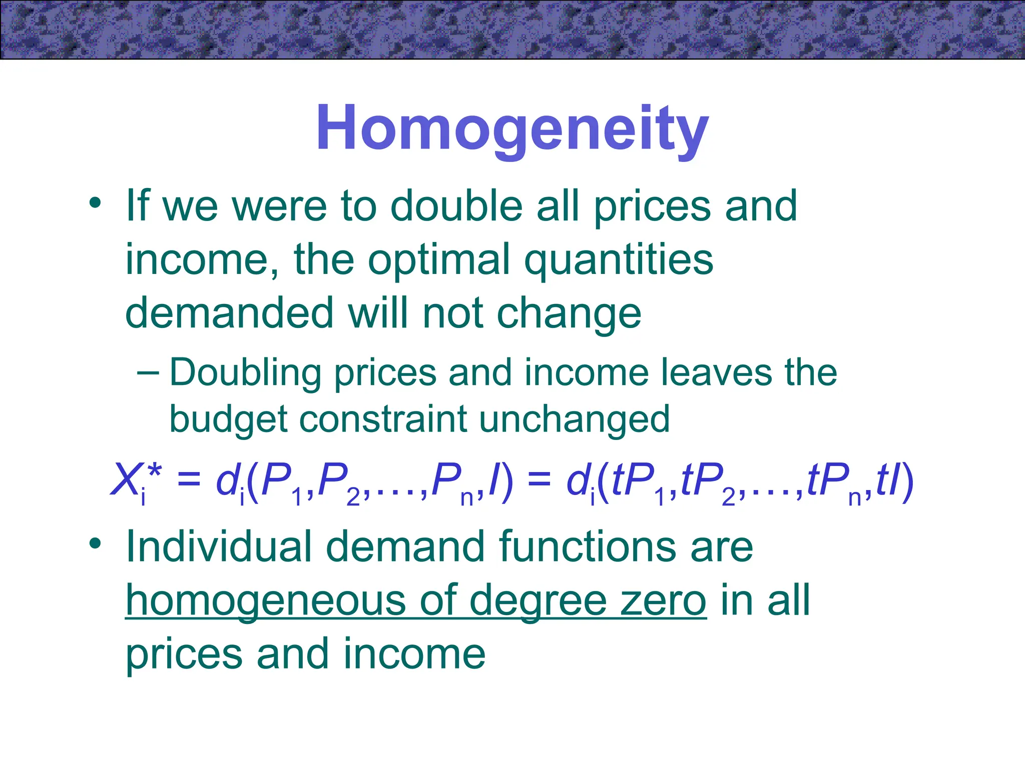
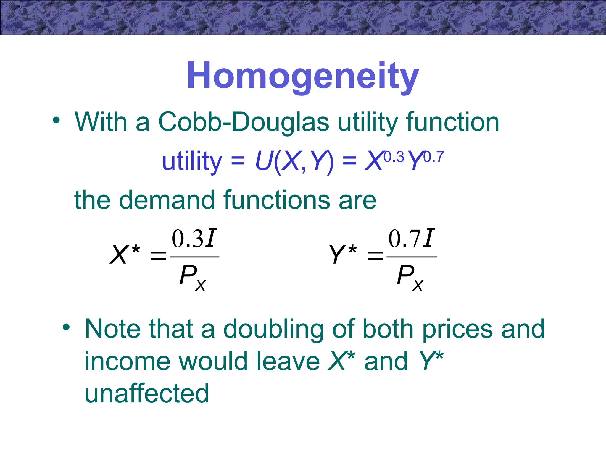
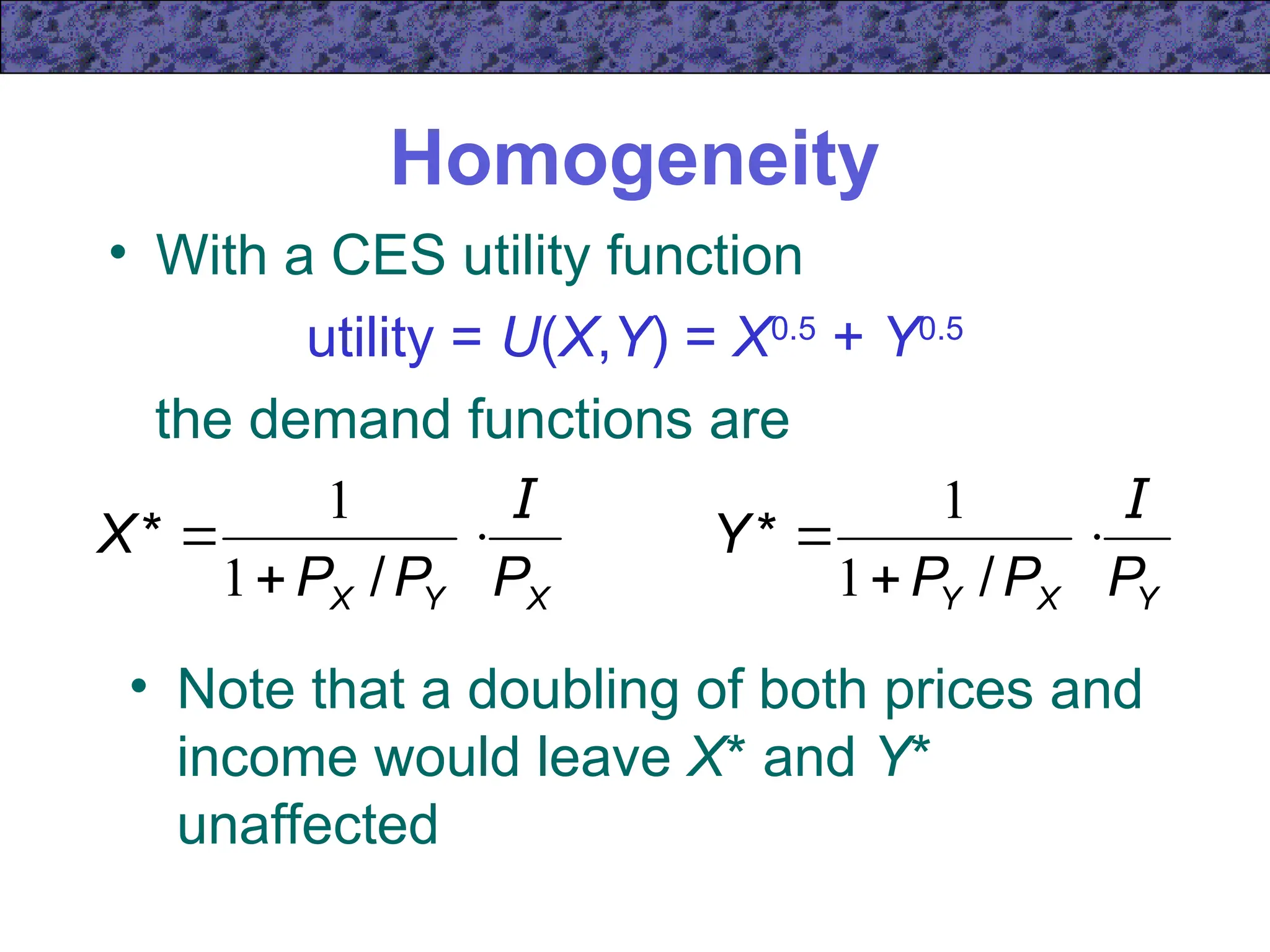
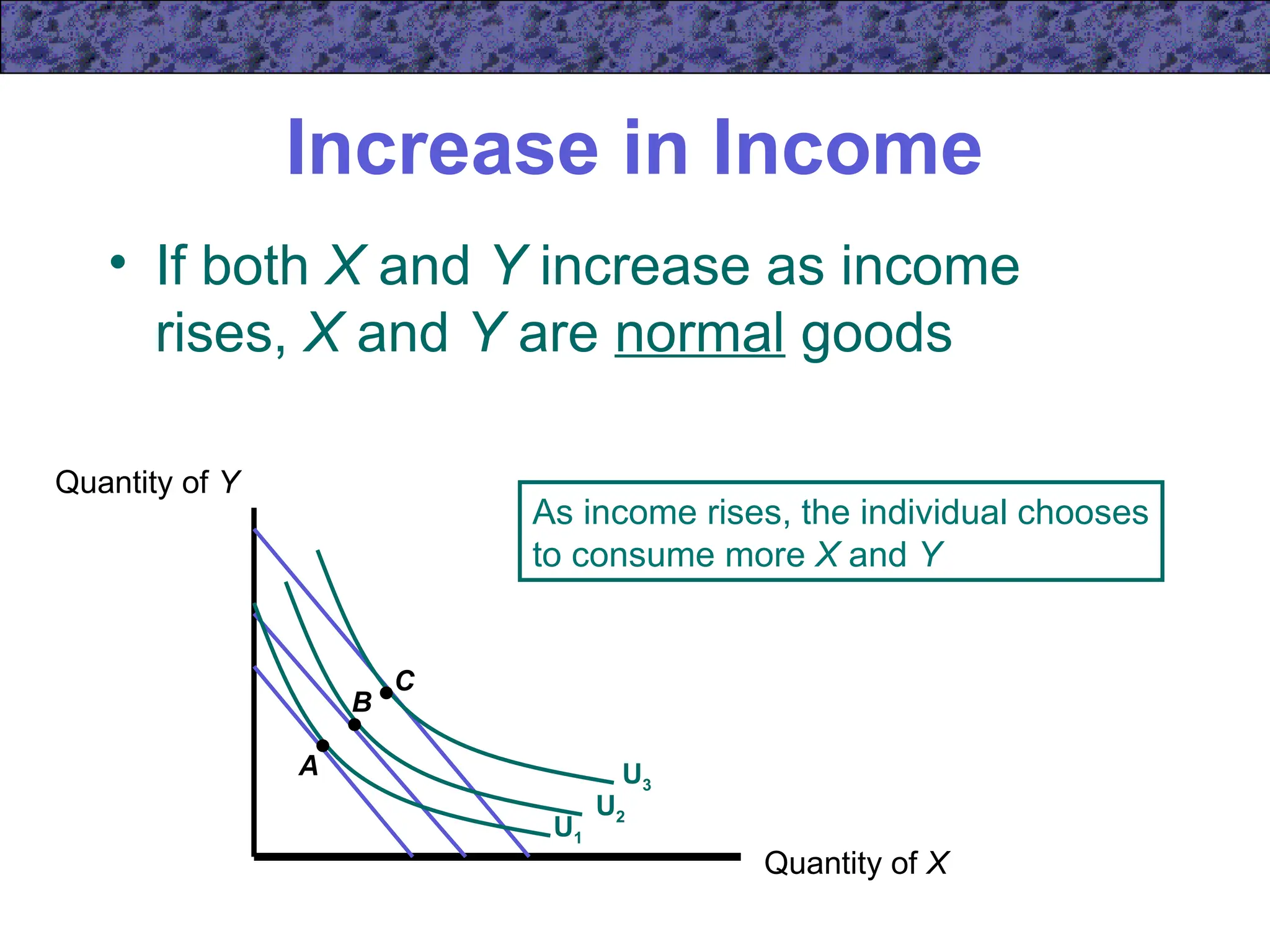
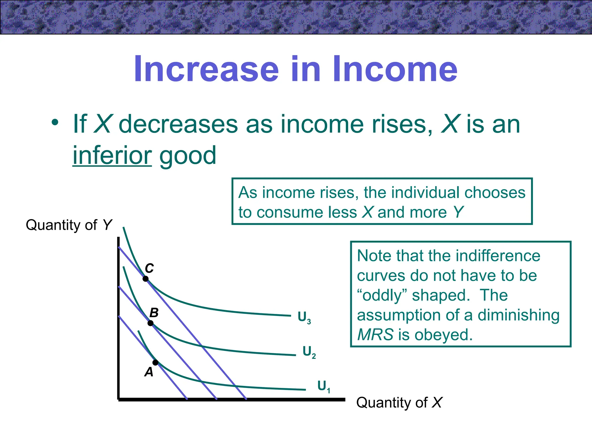
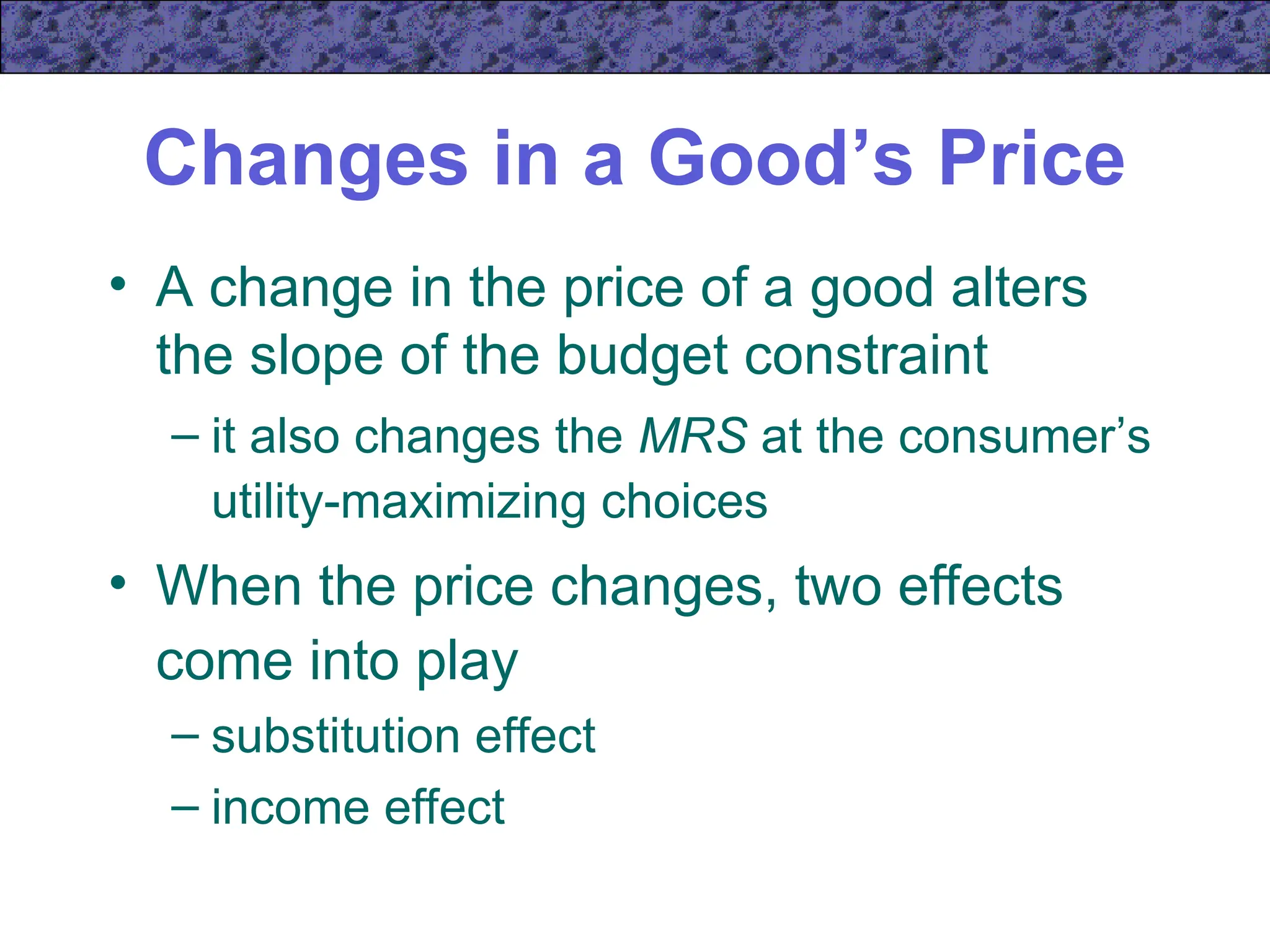
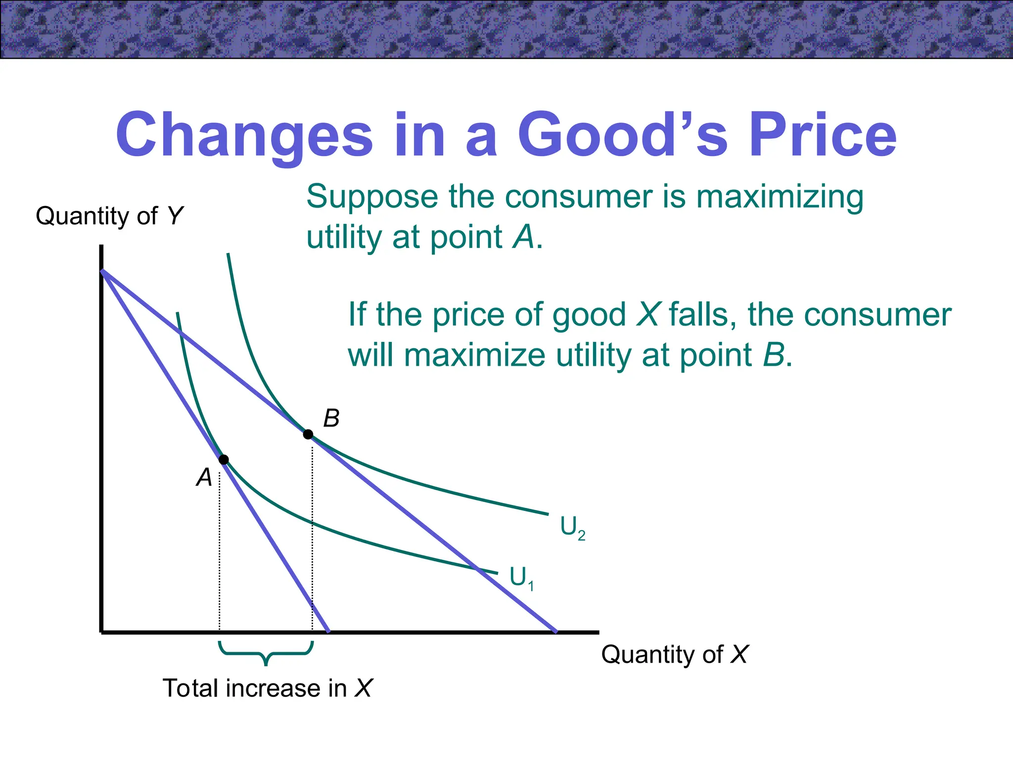
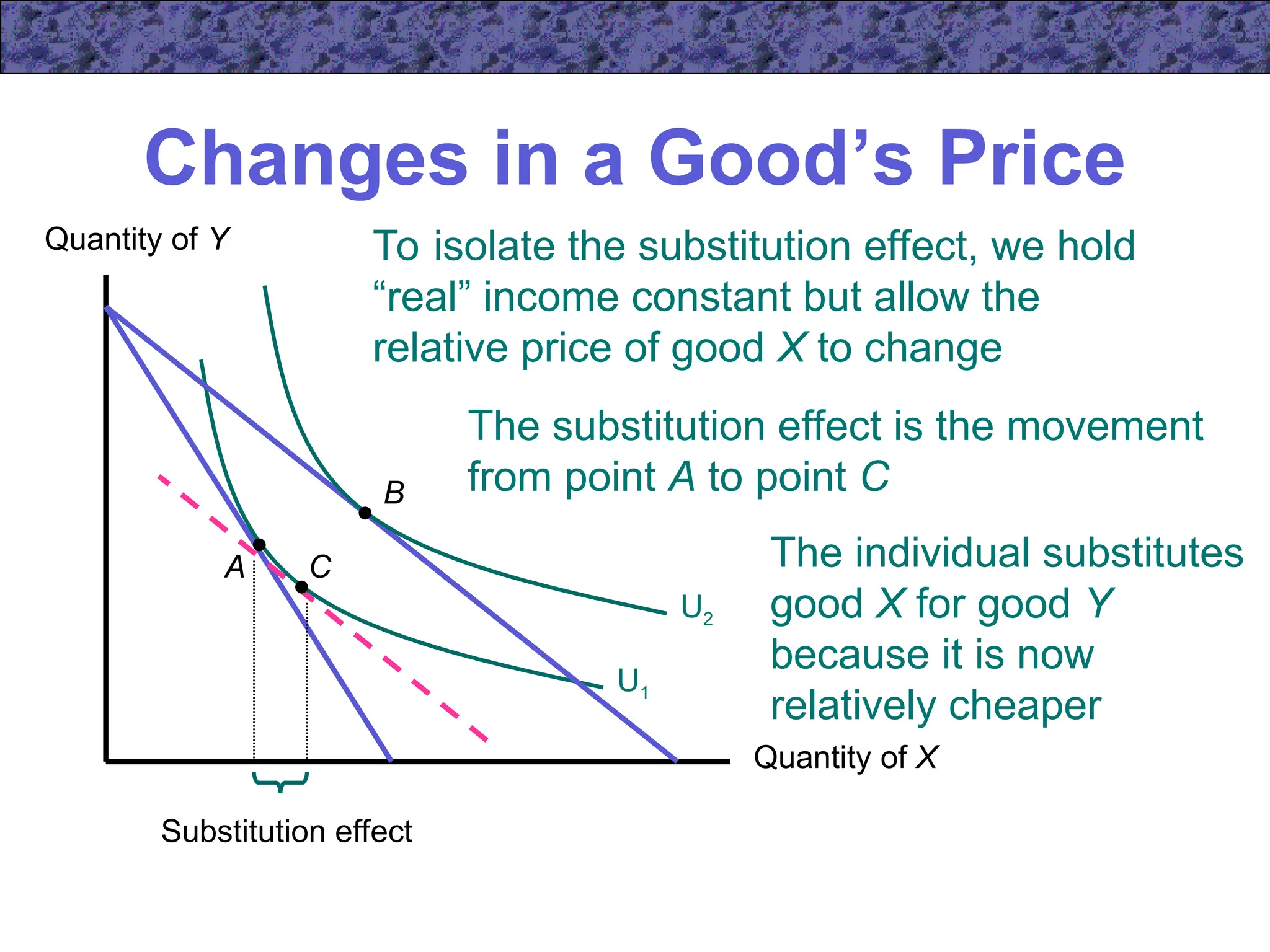
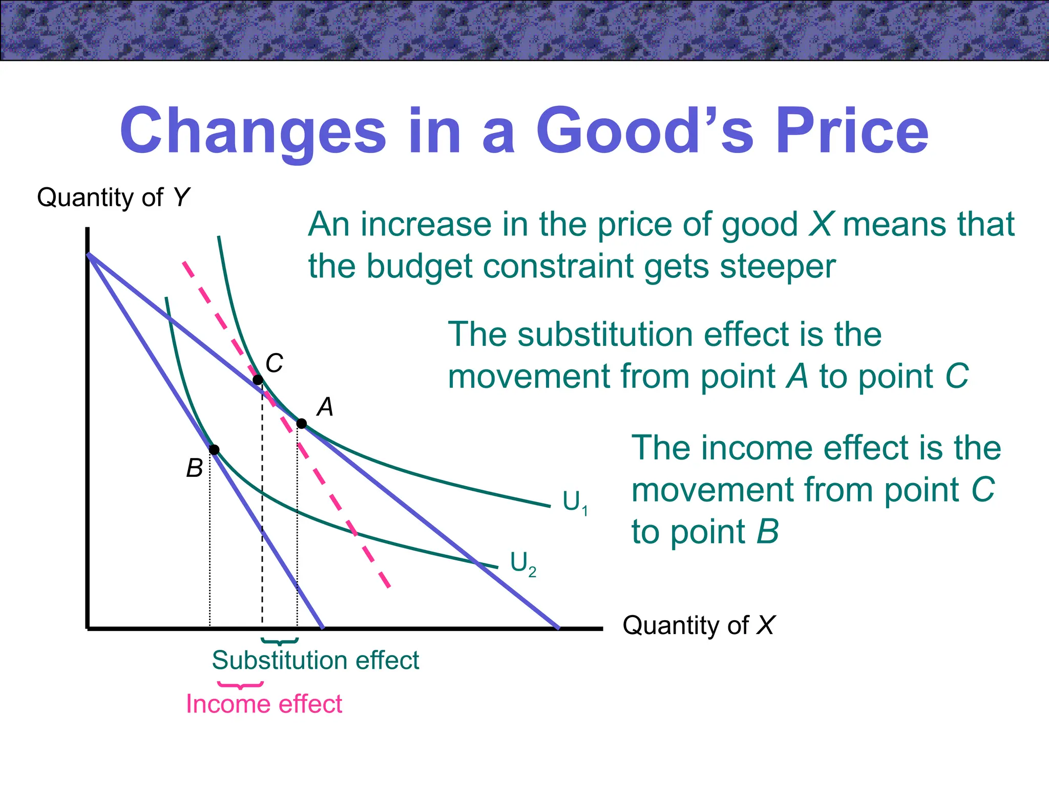
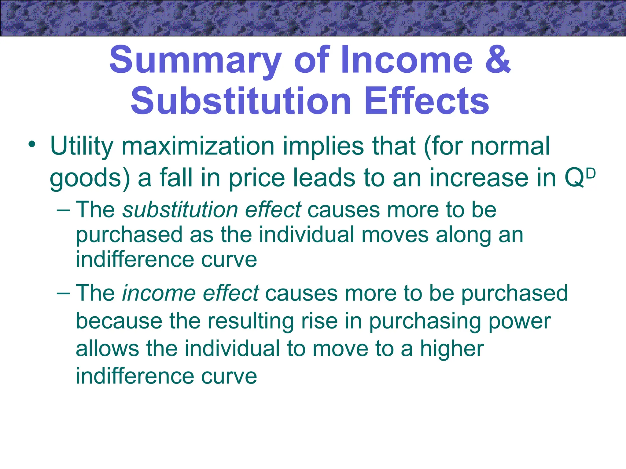
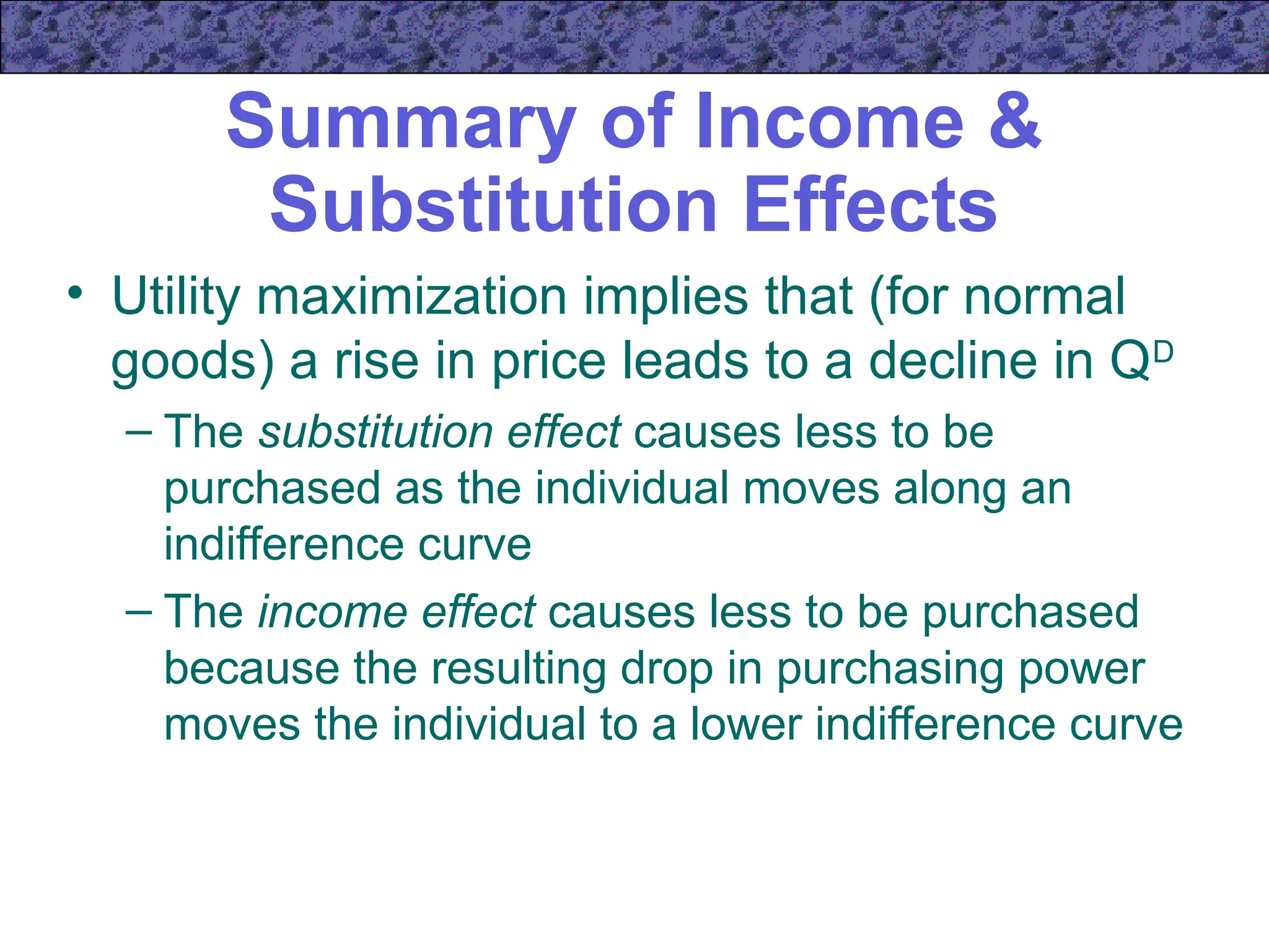
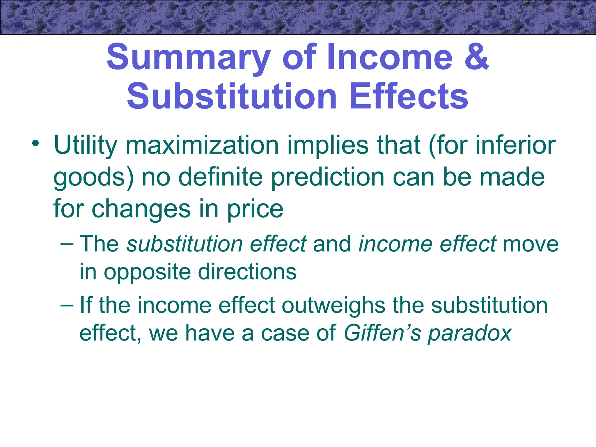
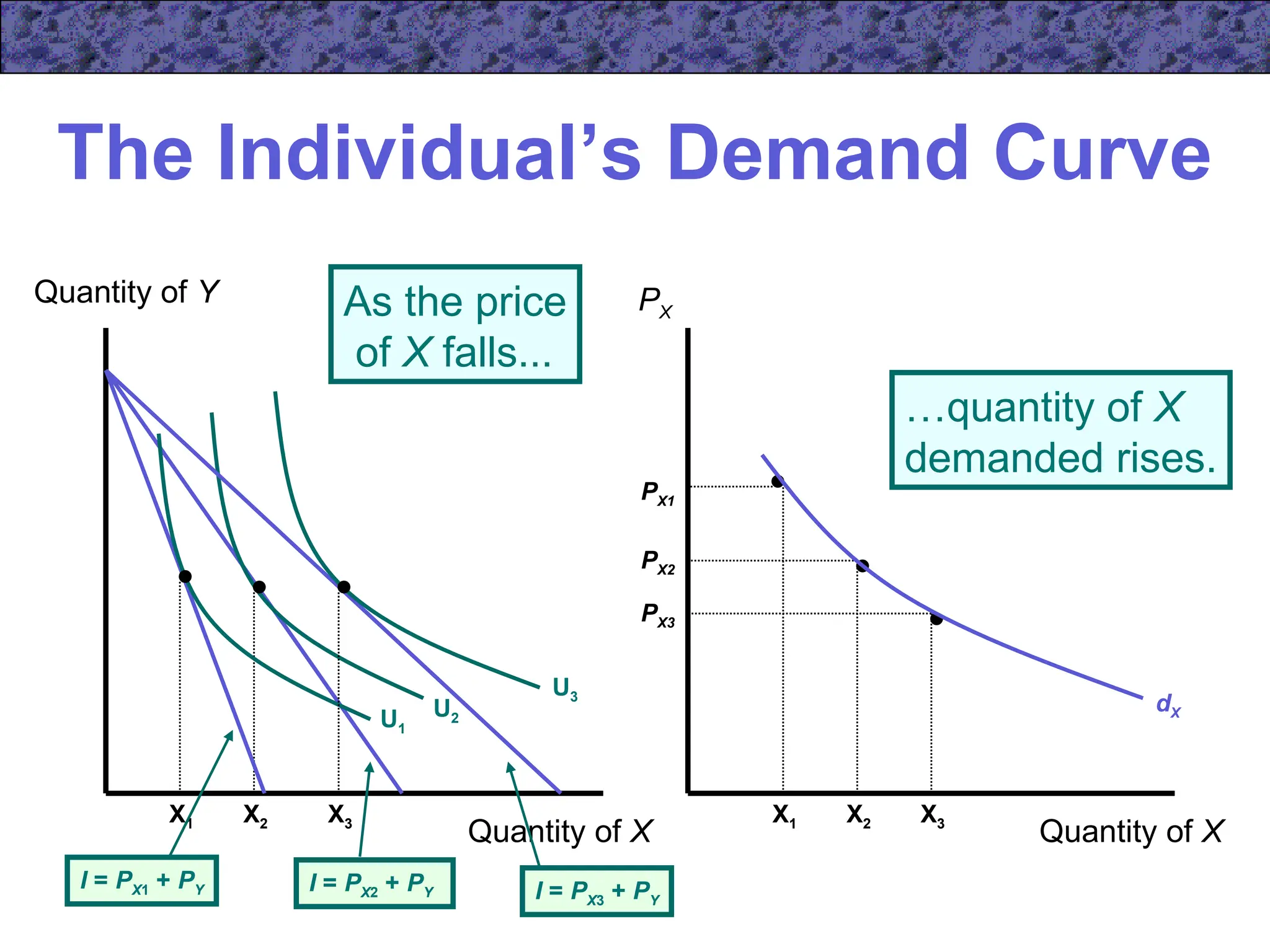
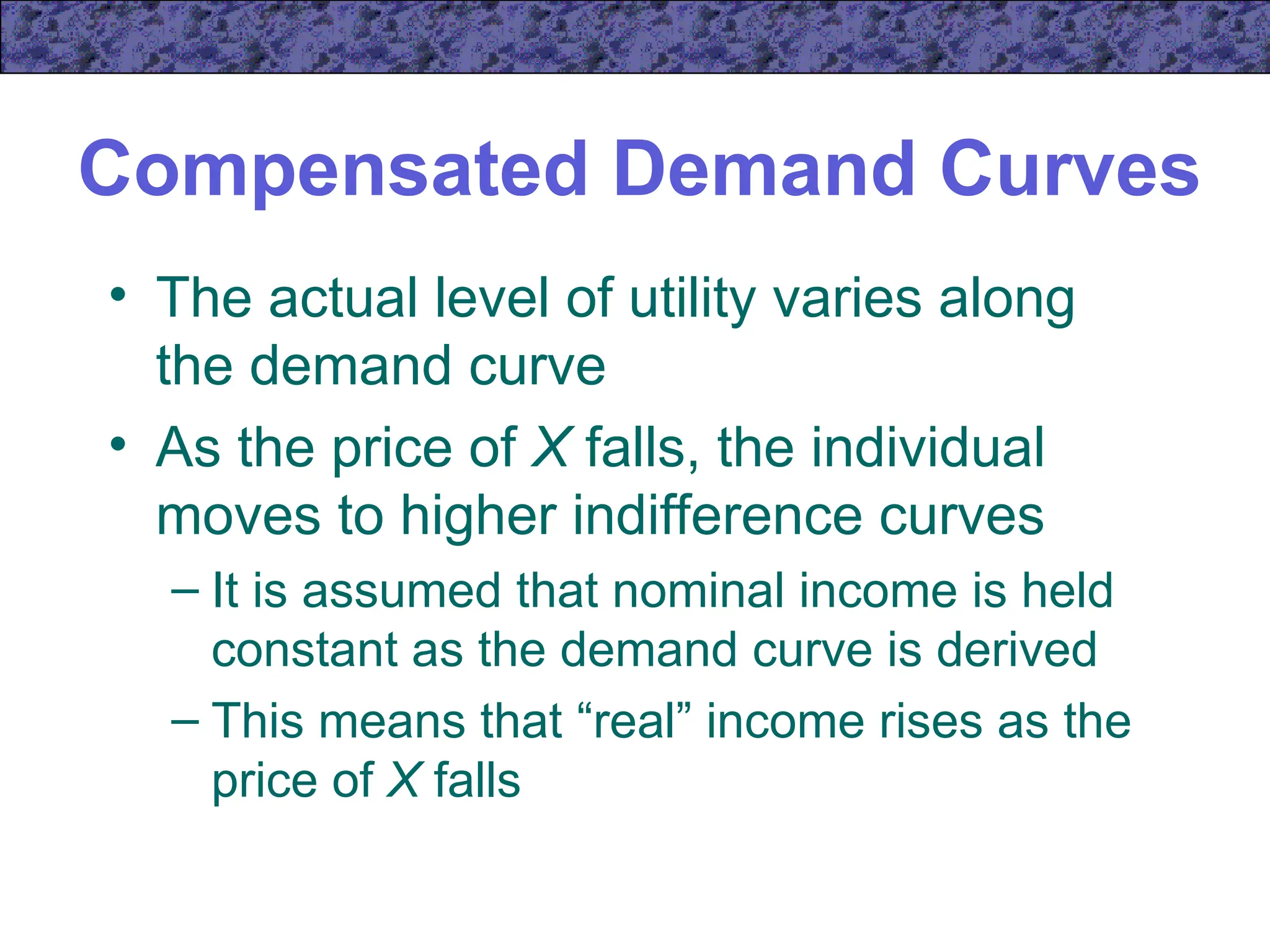
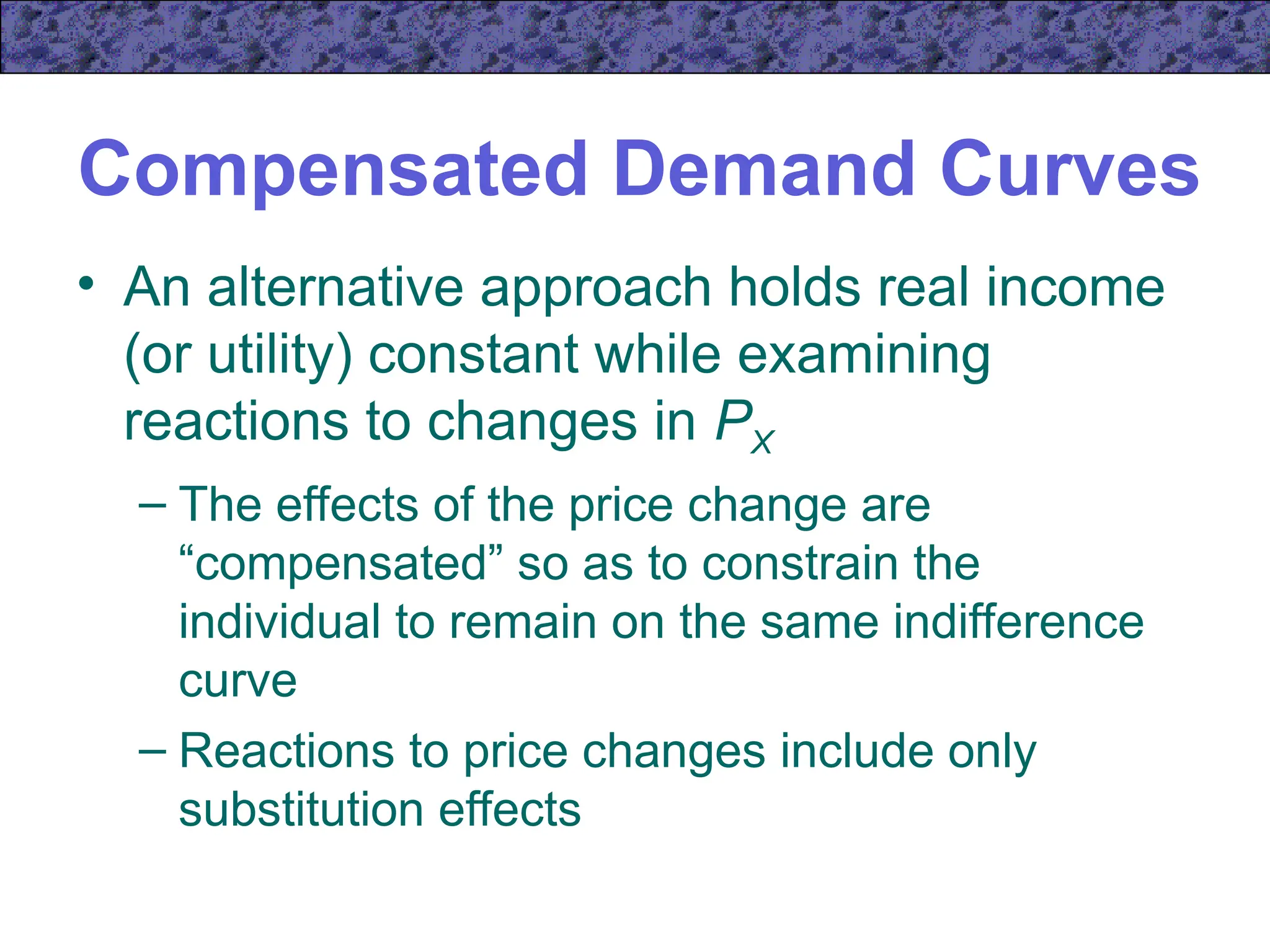
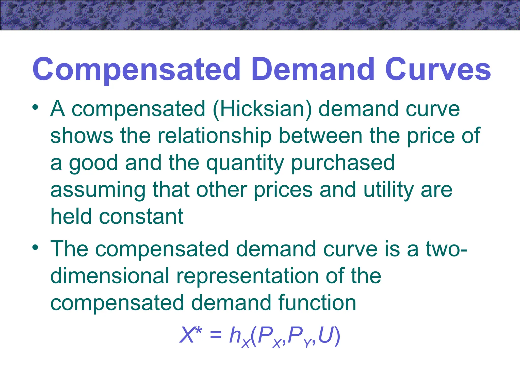
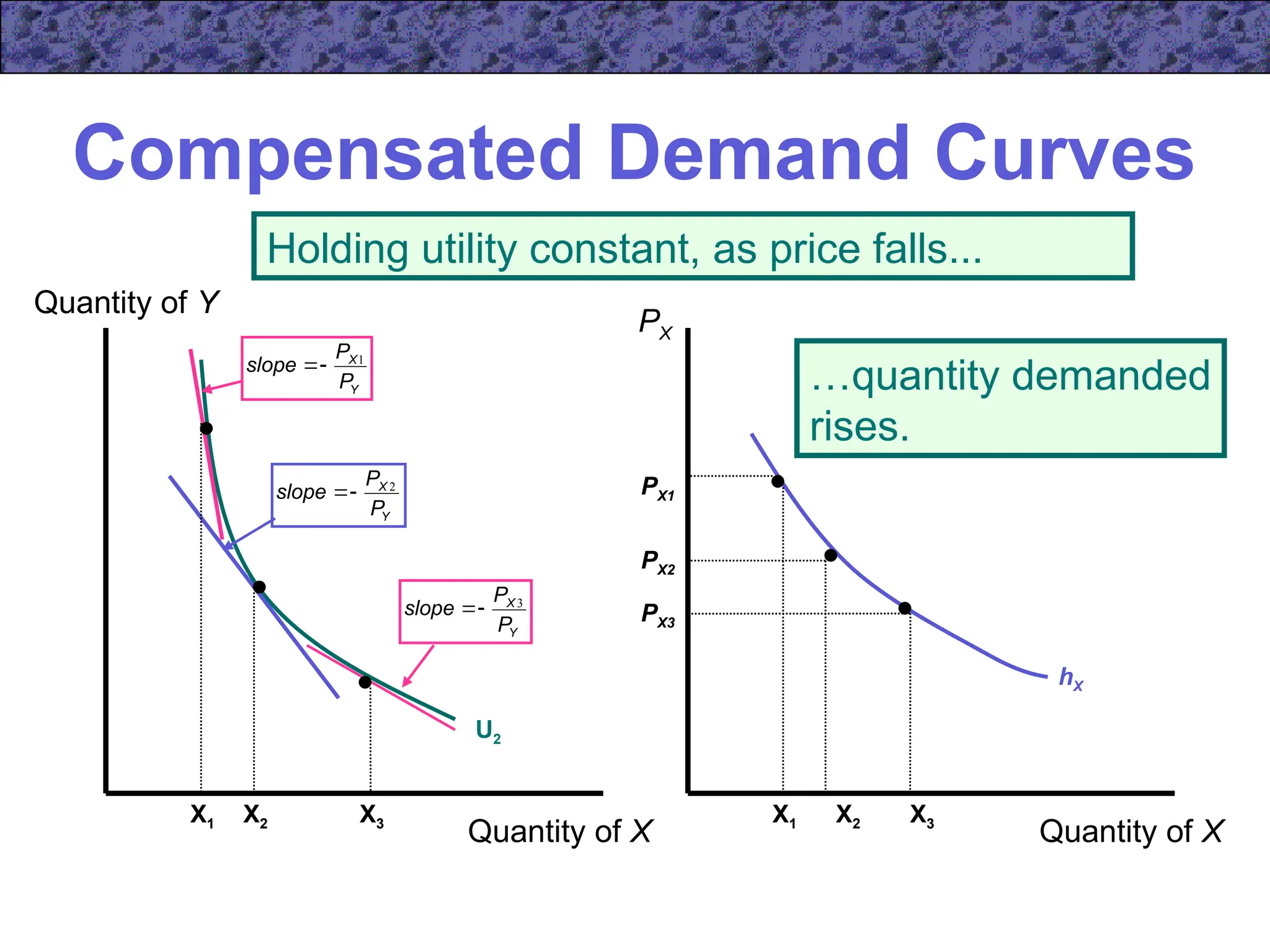
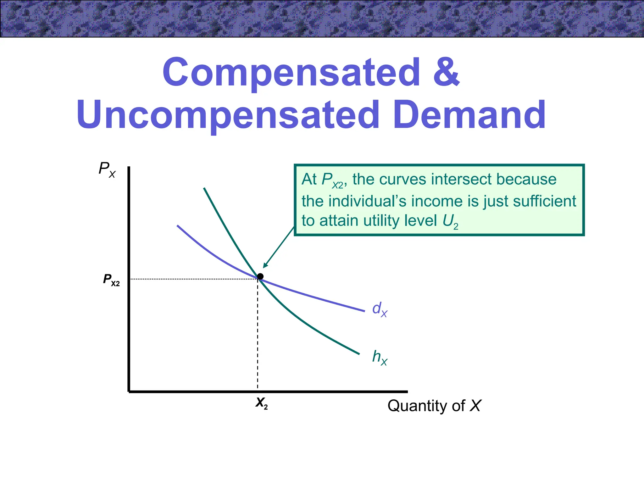
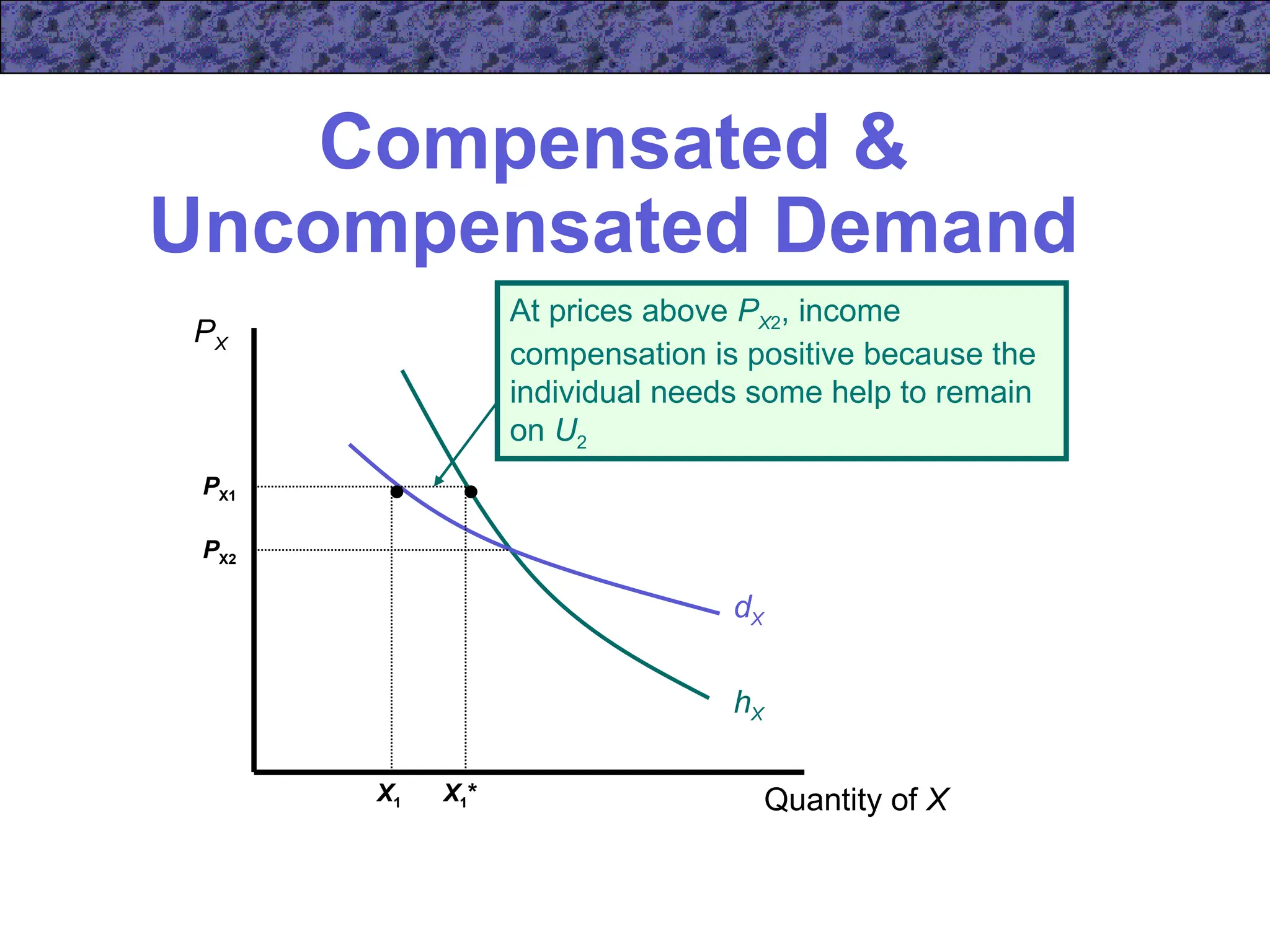
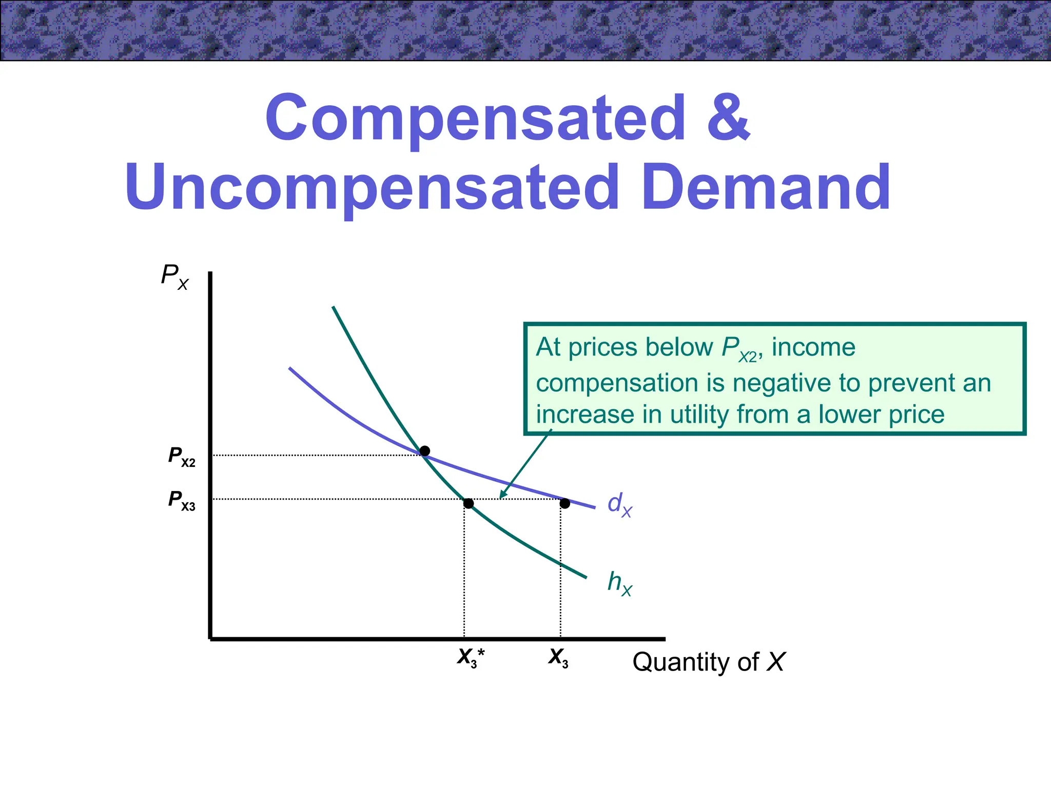
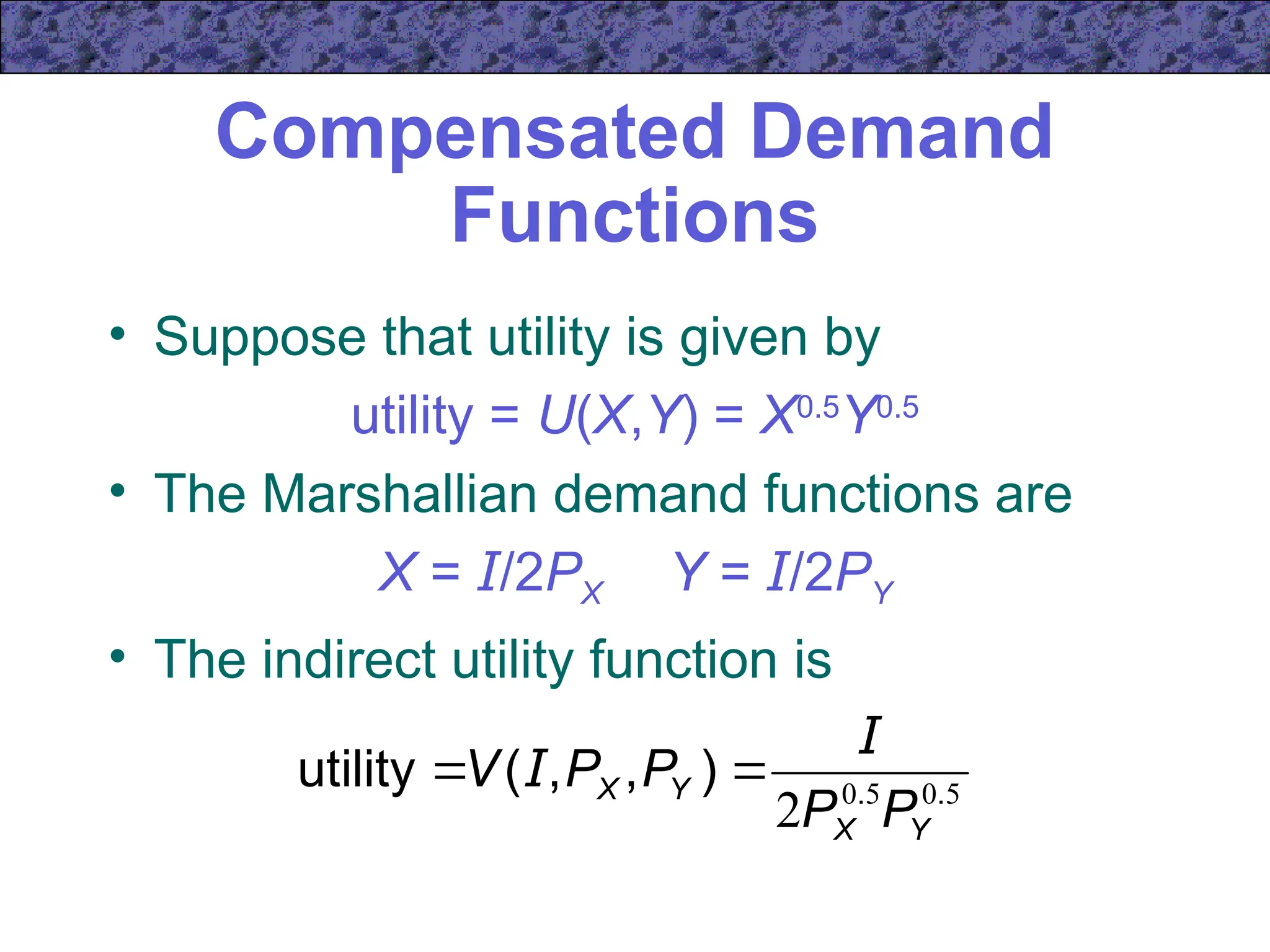
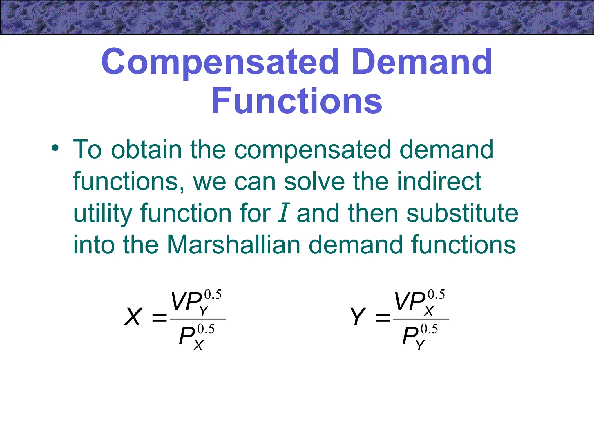
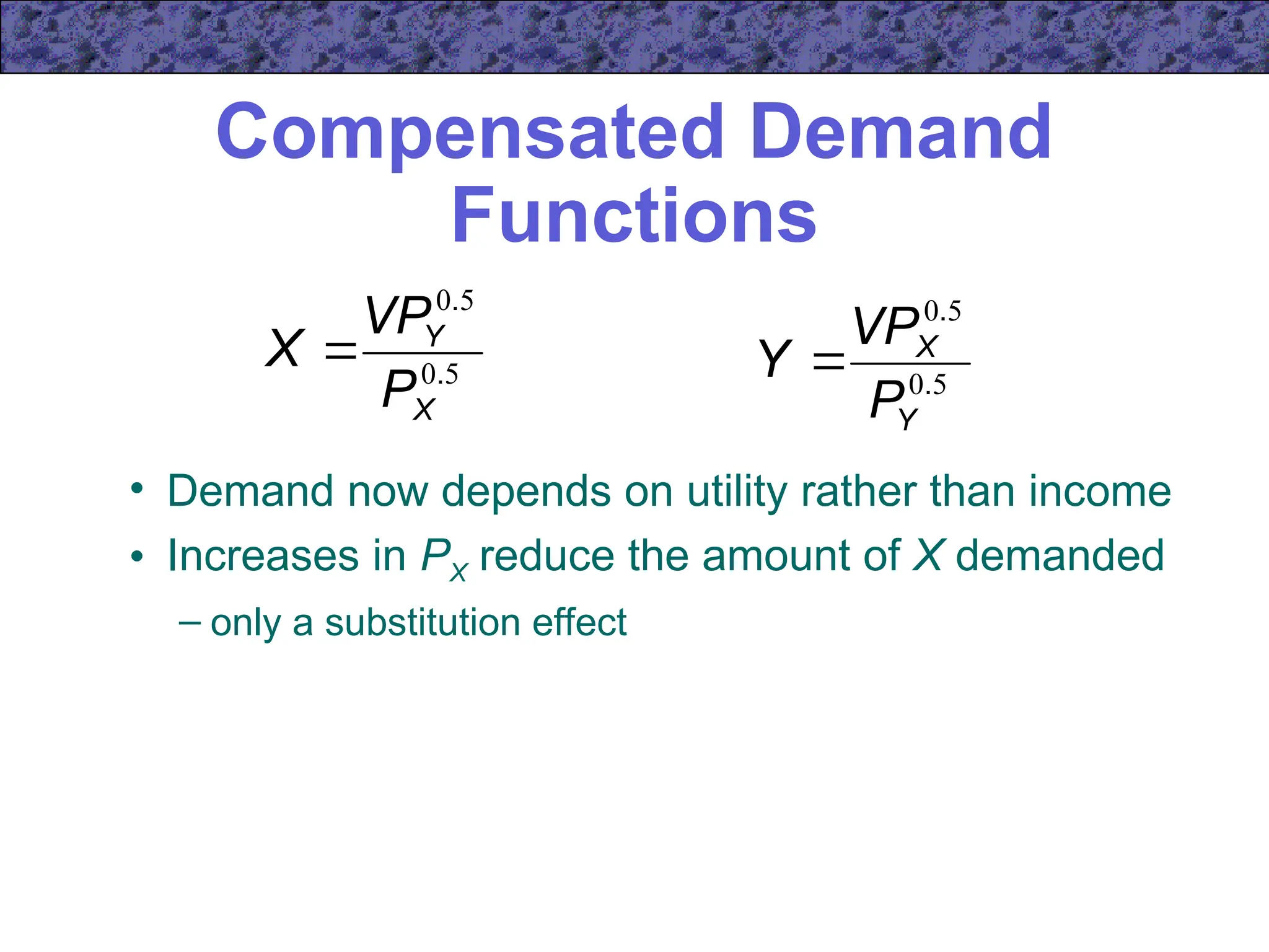
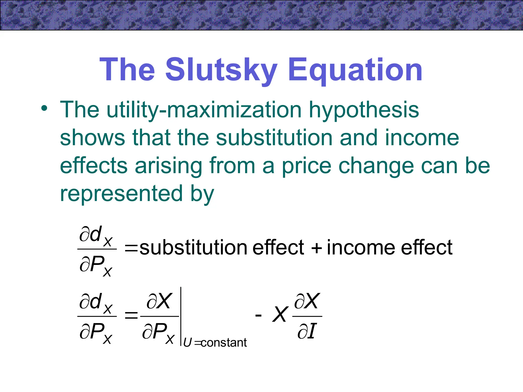
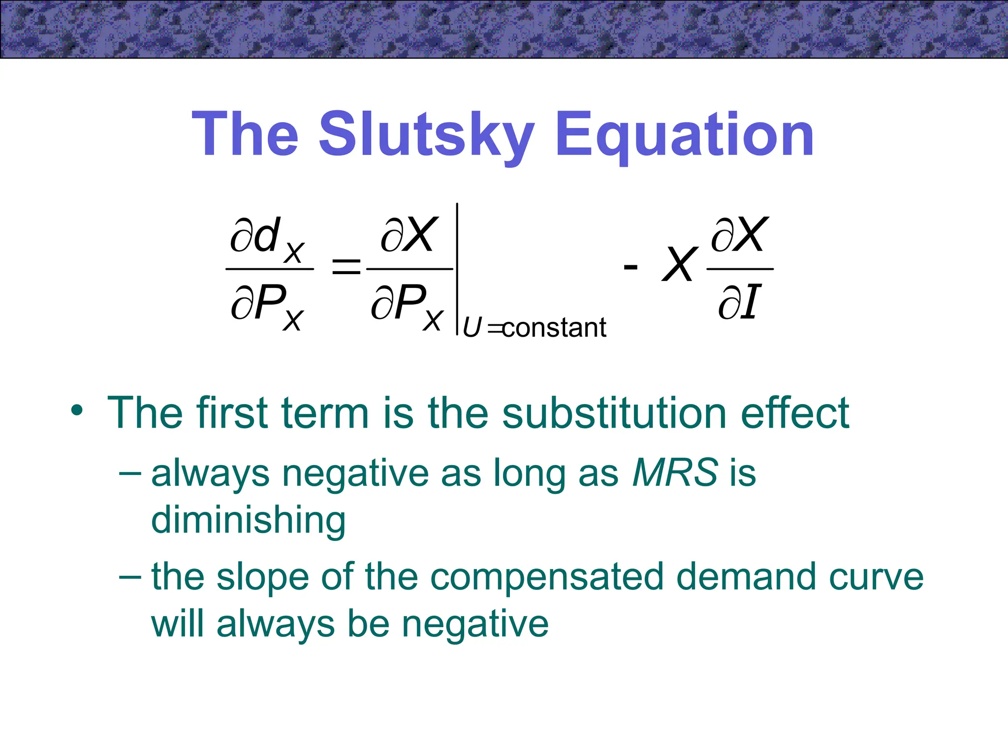
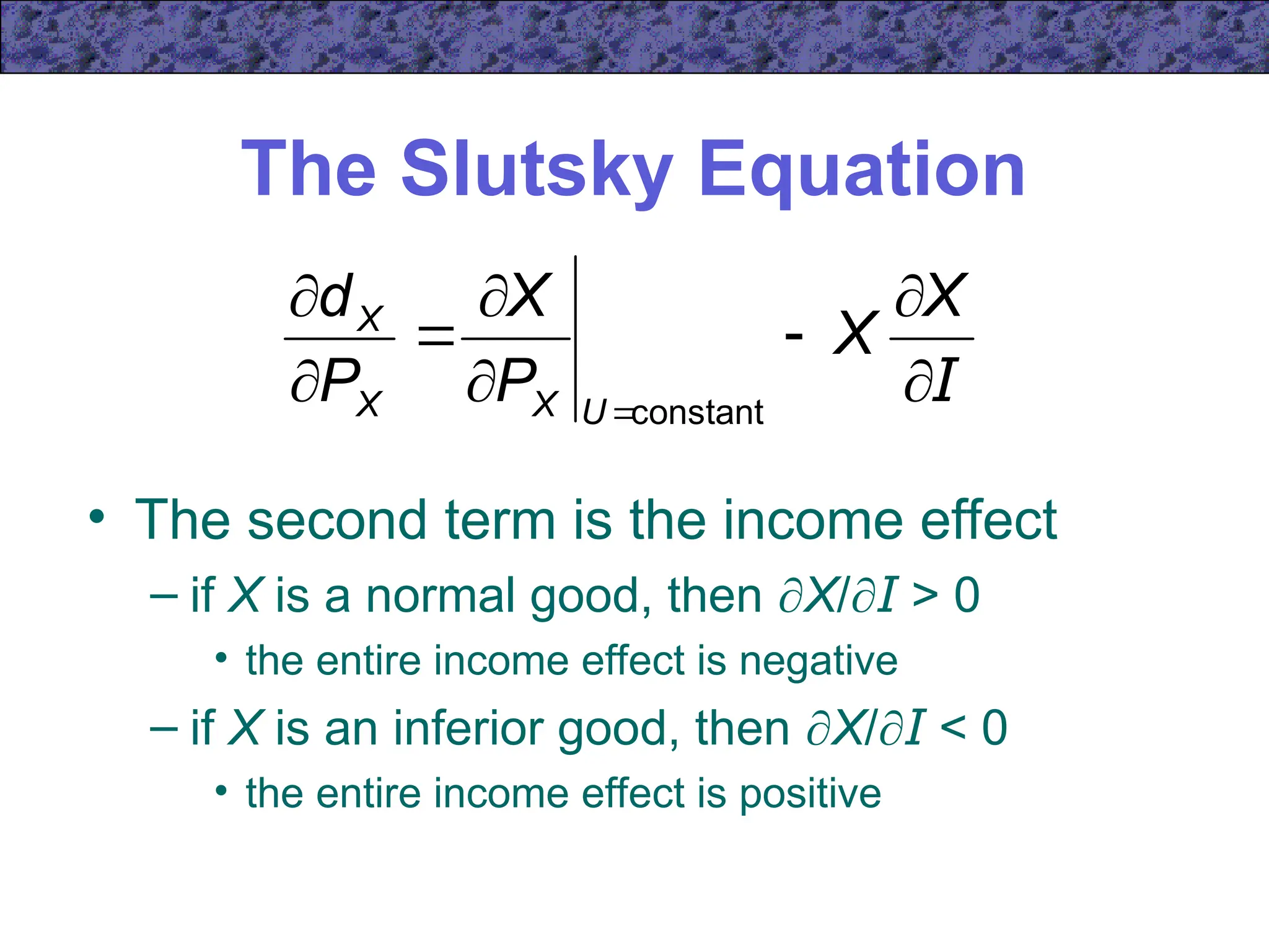
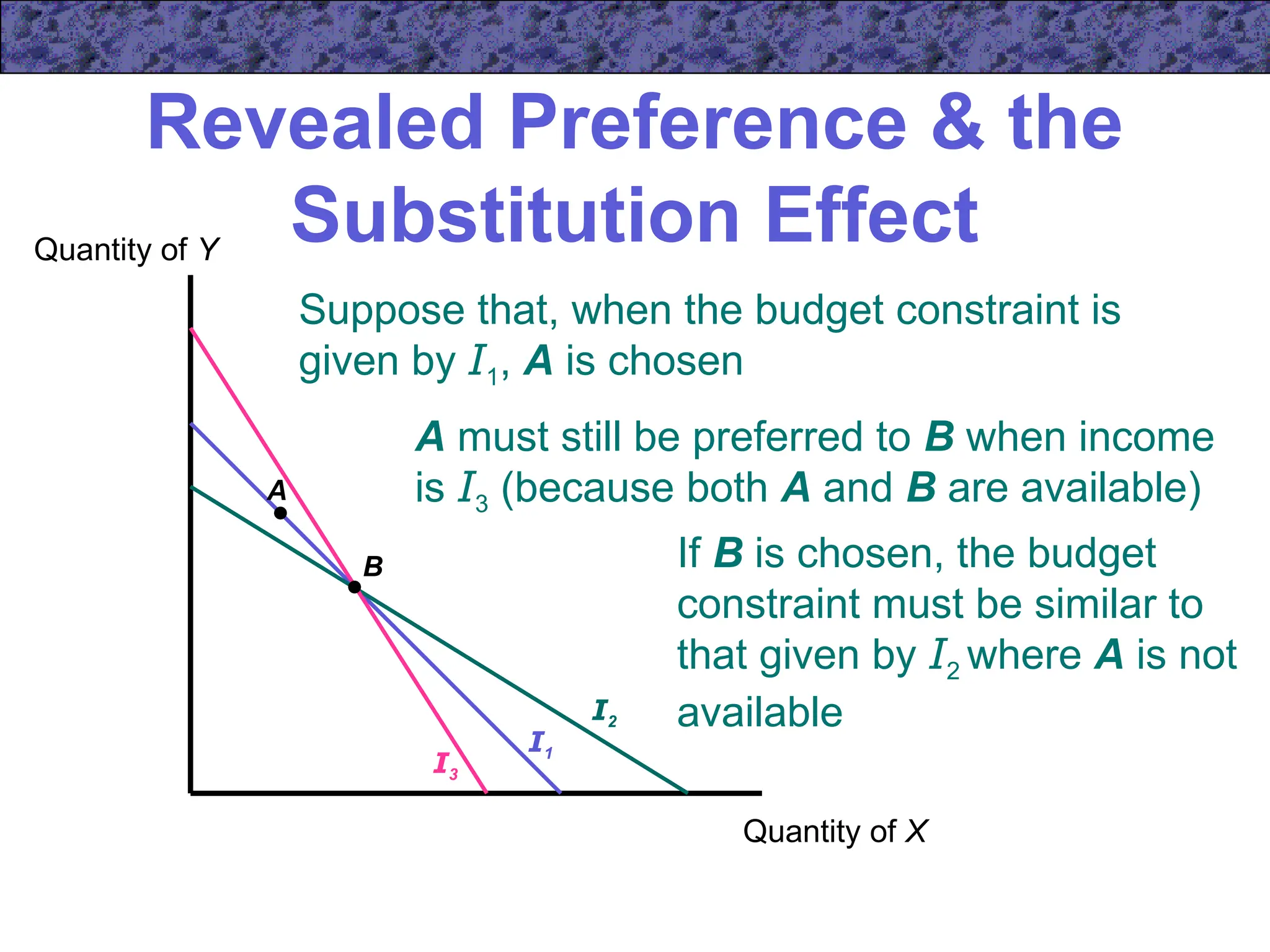
Chapter 5 focuses on income and substitution effects in microeconomic theory, detailing how changes in income and prices alter consumer behavior and demand functions. It introduces key concepts such as normal and inferior goods, Engel's Law, and the substitution and income effects during price changes. The chapter also covers demand curves, compensated demand functions, and the Slutsky equation, highlighting how consumer choices vary as prices and incomes fluctuate.

1. Chapter 5
INCOME AND SUBSTITUTION
EFFECTS
Copyright ©2002 by South-Western, a division of Thomson Learning. All rights reserved.
MICROECONOMIC THEORY
BASIC PRINCIPLES AND EXTENSIONS
EIGHTH EDITION
WALTER NICHOLSON

2. Demand Functions
• The optimal levels of X1,X2,…,Xn can be
expressed as functions of all prices and income
• These can be expressed as n demand
functions:
X1* = d1(P1,P2,…,Pn,I)
X2* = d2(P1,P2,…,Pn,I)
•
•
•
Xn* = dn(P1,P2,…,Pn,I)

3. Homogeneity
• If we were to double all prices and
income, the optimal quantities
demanded will not change
– Doubling prices and income leaves the
budget constraint unchanged
Xi* = di(P1,P2,…,Pn,I) = di(tP1,tP2,…,tPn,tI)
• Individual demand functions are
homogeneous of degree zero in all
prices and income

4. Homogeneity
• With a Cobb-Douglas utility function
utility = U(X,Y) = X0.3
Y0.7
the demand functions are
• Note that a doubling of both prices and
income would leave X* and Y*
unaffected
X
P
X
I
3
0.
* 
X
P
Y
I
7
0.
* 

5. Homogeneity
• With a CES utility function
utility = U(X,Y) = X0.5
+ Y0.5
the demand functions are
• Note that a doubling of both prices and
income would leave X* and Y*
unaffected
X
Y
X P
P
P
X
I



/
*
1
1
Y
X
Y P
P
P
Y
I



/
*
1
1

6. Changes in Income
• An increase in income will cause the
budget constraint out in a parallel
manner
• Since PX/PY does not change, the MRS
will stay constant as the worker moves
to higher levels of satisfaction

7. Increase in Income
• If both X and Y increase as income
rises, X and Y are normal goods
Quantity of X
Quantity of Y
C
U3
B
U2
A
U1
As income rises, the individual chooses
to consume more X and Y

8. Increase in Income
• If X decreases as income rises, X is an
inferior good
Quantity of X
Quantity of Y
C
U3
As income rises, the individual chooses
to consume less X and more Y
Note that the indifference
curves do not have to be
“oddly” shaped. The
assumption of a diminishing
MRS is obeyed.
B
U2
A
U1

9. Normal and Inferior Goods
• A good Xi for which Xi/I  0 over
some range of income is a normal good
in that range
• A good Xi for which Xi/I < 0 over
some range of income is an inferior
good in that range

10. Engel’s Law
• Using Belgian data from 1857, Engel
found an empirical generalization about
consumer behavior
• The proportion of total expenditure
devoted to food declines as income rises
– food is a necessity whose consumption rises
less rapidly than income

11. Substitution & Income Effects
• Even if the individual remained on the same
indifference curve when the price changes,
his optimal choice will change because the
MRS must equal the new price ratio
– the substitution effect
• The price change alters the individual’s “real”
income and therefore he must move to a new
indifference curve
– the income effect

12. Changes in a Good’s Price
• A change in the price of a good alters
the slope of the budget constraint
– it also changes the MRS at the consumer’s
utility-maximizing choices
• When the price changes, two effects
come into play
– substitution effect
– income effect

13. Changes in a Good’s Price
Quantity of X
Quantity of Y
U1
A
Suppose the consumer is maximizing
utility at point A.
U2
B
If the price of good X falls, the consumer
will maximize utility at point B.
Total increase in X

14. Changes in a Good’s Price
U1
U2
Quantity of X
Quantity of Y
A
B
To isolate the substitution effect, we hold
“real” income constant but allow the
relative price of good X to change
C
Substitution effect
The substitution effect is the movement
from point A to point C
The individual substitutes
good X for good Y
because it is now
relatively cheaper

15. Changes in a Good’s Price
U1
U2
Quantity of X
Quantity of Y
A
B
The income effect occurs because the
individual’s “real” income changes when
the price of good X changes
C
Income effect
The income effect is the movement
from point C to point B
If X is a normal good,
the individual will buy
more because “real”
income increased

16. Changes in a Good’s Price
U2
U1
Quantity of X
Quantity of Y
B
A
An increase in the price of good X means that
the budget constraint gets steeper
C
The substitution effect is the
movement from point A to point C
Substitution effect
Income effect
The income effect is the
movement from point C
to point B

17. Price Changes for
Normal Goods
• If a good is normal, substitution and
income effects reinforce one another
– When price falls, both effects lead to a rise
in QD
– When price rises, both effects lead to a drop
in QD

18. Price Changes for
Inferior Goods
• If a good is inferior, substitution and income
effects move in opposite directions
• The combined effect is indeterminate
– When price rises, the substitution effect leads to
a drop in QD
, but the income effect leads to a
rise in QD
– When price falls, the substitution effect leads to
a rise in QD
, but the income effect leads to a fall
in QD

19. Giffen’s Paradox
• If the income effect of a price change is
strong enough, there could be a positive
relationship between price and QD
– An increase in price leads to a drop in real
income
– Since the good is inferior, a drop in income
causes QD
to rise
• Thus, a rise in price leads to a rise in QD

20. Summary of Income &
Substitution Effects
• Utility maximization implies that (for normal
goods) a fall in price leads to an increase in QD
– The substitution effect causes more to be
purchased as the individual moves along an
indifference curve
– The income effect causes more to be purchased
because the resulting rise in purchasing power
allows the individual to move to a higher
indifference curve

21. Summary of Income &
Substitution Effects
• Utility maximization implies that (for normal
goods) a rise in price leads to a decline in QD
– The substitution effect causes less to be
purchased as the individual moves along an
indifference curve
– The income effect causes less to be purchased
because the resulting drop in purchasing power
moves the individual to a lower indifference curve

22. Summary of Income &
Substitution Effects
• Utility maximization implies that (for inferior
goods) no definite prediction can be made
for changes in price
– The substitution effect and income effect move
in opposite directions
– If the income effect outweighs the substitution
effect, we have a case of Giffen’s paradox

23. The Individual’s Demand Curve
• An individual’s demand for X1 depends
on preferences, all prices, and income:
X1* = d1(P1,P2,…,Pn,I)
• It may be convenient to graph the
individual’s demand for X1 assuming
that income and the prices of other
goods are held constant

24. The Individual’s Demand Curve
Quantity of Y
Quantity of X Quantity of X
PX
X2
PX2
U2
X2
I = PX2 + PY
X1
PX1
U1
X1
I = PX1 + PY
X3
PX3
X3
U3
I = PX3 + PY
As the price
of X falls...
dX
…quantity of X
demanded rises.

25. The Individual’s Demand Curve
• An individual demand curve shows the
relationship between the price of a good
and the quantity of that good purchased by
an individual assuming that all other
determinants of demand are held constant

26. Shifts in the Demand Curve
• Three factors are held constant when a
demand curve is derived
– income
– prices of other goods
– the individual’s preferences
• If any of these factors change, the
demand curve will shift to a new position

27. Shifts in the Demand Curve
• A movement along a given demand
curve is caused by a change in the price
of the good
– called a change in quantity demanded
• A shift in the demand curve is caused by
a change in income, prices of other
goods, or preferences
– called a change in demand

28. Compensated Demand Curves
• The actual level of utility varies along
the demand curve
• As the price of X falls, the individual
moves to higher indifference curves
– It is assumed that nominal income is held
constant as the demand curve is derived
– This means that “real” income rises as the
price of X falls

29. Compensated Demand Curves
• An alternative approach holds real income
(or utility) constant while examining
reactions to changes in PX
– The effects of the price change are
“compensated” so as to constrain the
individual to remain on the same indifference
curve
– Reactions to price changes include only
substitution effects

30. Compensated Demand Curves
• A compensated (Hicksian) demand curve
shows the relationship between the price of
a good and the quantity purchased
assuming that other prices and utility are
held constant
• The compensated demand curve is a two-
dimensional representation of the
compensated demand function
X* = hX(PX,PY,U)

31. hX
…quantity demanded
rises.
Compensated Demand Curves
Quantity of Y
Quantity of X Quantity of X
PX
U2
X2
PX2
X2
Y
X
P
P
slope 2


X1
PX1
Y
X
P
P
slope 1


X1 X3
PX3
Y
X
P
P
slope 3


X3
Holding utility constant, as price falls...

32. Compensated &
Uncompensated Demand
Quantity of X
PX
dX
hX
X2
PX2
At PX2, the curves intersect because
the individual’s income is just sufficient
to attain utility level U2

33. Compensated &
Uncompensated Demand
Quantity of X
PX
dX
hX
PX2
X1*
X1
PX1
At prices above PX2, income
compensation is positive because the
individual needs some help to remain
on U2

34. Compensated &
Uncompensated Demand
Quantity of X
PX
dX
hX
PX2
X3* X3
PX3
At prices below PX2, income
compensation is negative to prevent an
increase in utility from a lower price

35. Compensated &
Uncompensated Demand
• For a normal good, the compensated
demand curve is less responsive to price
changes than is the uncompensated
demand curve
– the uncompensated demand curve reflects
both income and substitution effects
– the compensated demand curve reflects only
substitution effects

36. Compensated Demand
Functions
• Suppose that utility is given by
utility = U(X,Y) = X0.5
Y0.5
• The Marshallian demand functions are
X = I/2PX Y = I/2PY
• The indirect utility function is
5
0
5
0
2 .
.
)
,
,
(
utility
Y
X
Y
X
P
P
P
P
V
I
I 


37. Compensated Demand
Functions
• To obtain the compensated demand
functions, we can solve the indirect
utility function for I and then substitute
into the Marshallian demand functions
5
0
5
0
.
.
X
Y
P
VP
X  5
0
5
0
.
.
Y
X
P
VP
Y 

38. Compensated Demand
Functions
• Demand now depends on utility rather than income
• Increases in PX reduce the amount of X demanded
– only a substitution effect
5
0
5
0
.
.
X
Y
P
VP
X 
5
0
5
0
.
.
Y
X
P
VP
Y 

39. A Mathematical Examination
of a Change in Price
• Our goal is to examine how the demand for
good X changes when PX changes
dX/PX
• Differentiation of the first-order conditions
from utility maximization can be performed
to solve for this derivative
• However, this approach is cumbersome and
provides little economic insight

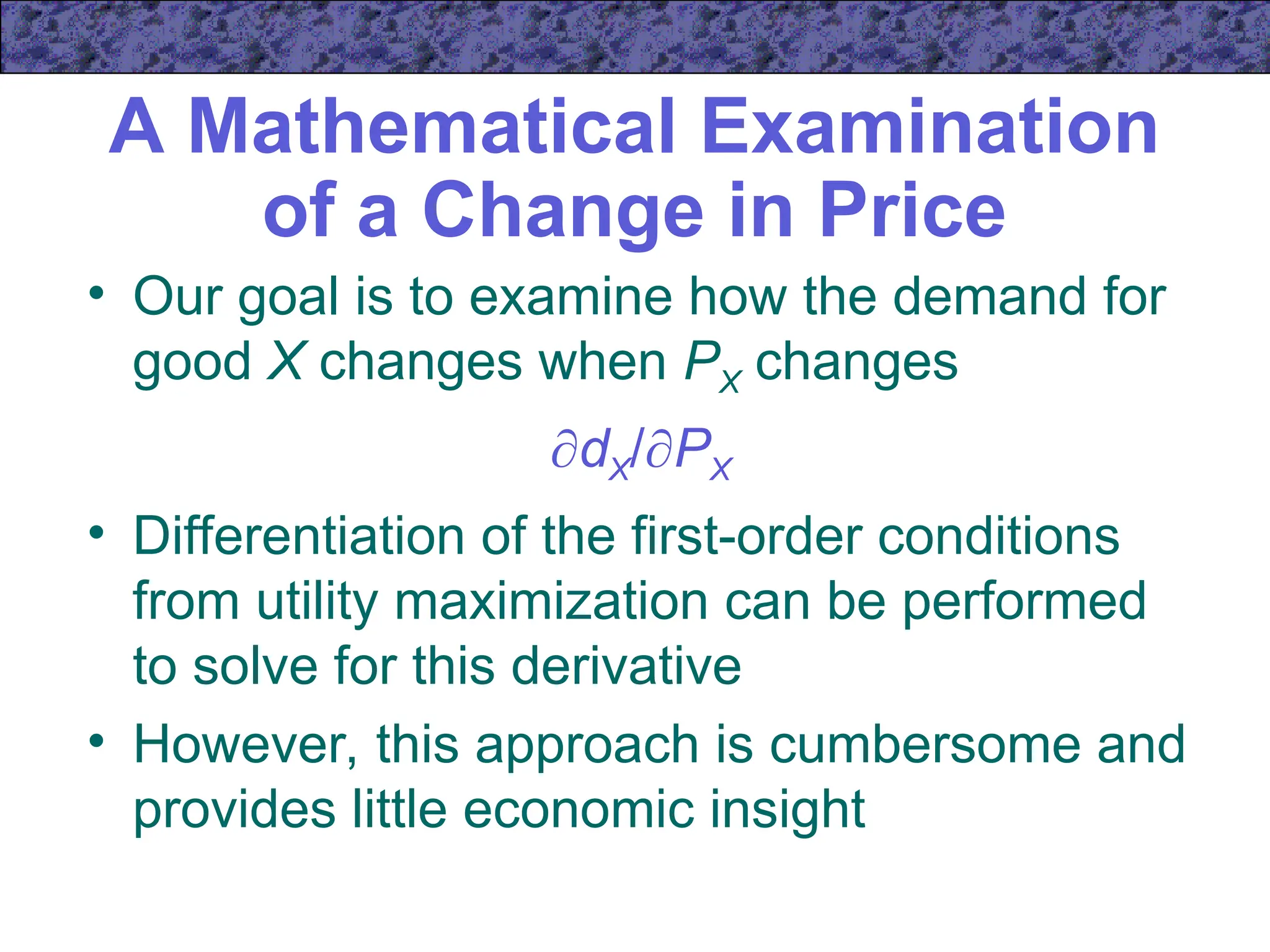
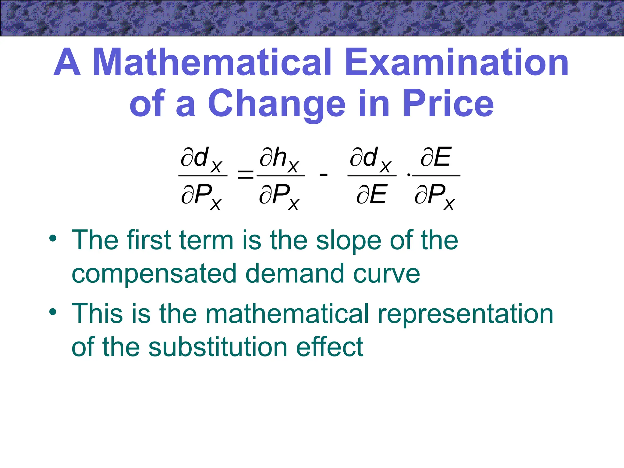
40. A Mathematical Examination
of a Change in Price
• Instead, we will use an indirect approach
• Remember the expenditure function
minimum expenditure = E(PX,PY,U)
• Then, by definition
hX (PX,PY,U) = dX [PX,PY,E(PX,PY,U)]
– Note that the two demand functions are equal
when income is exactly what is needed to attain
the required utility level

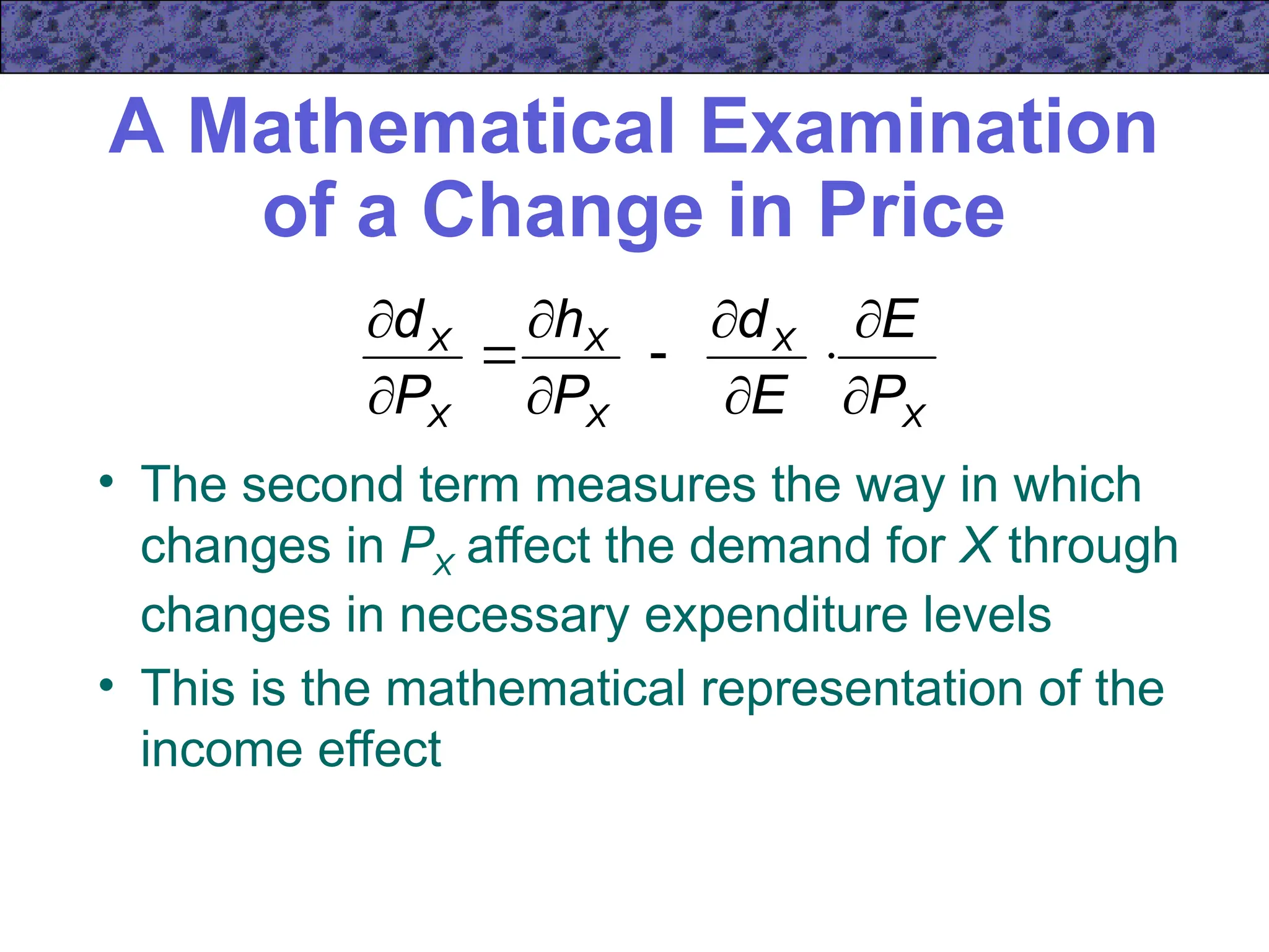
41. A Mathematical Examination
of a Change in Price
• We can differentiate the compensated
demand function and get
hX (PX,PY,U) = dX [PX,PY,E(PX,PY,U)]
X
X
X
X
X
X
P
E
E
d
P
d
P
h











X
X
X
X
X
X
P
E
E
d
P
h
P
d












42. A Mathematical Examination
of a Change in Price
• The first term is the slope of the
compensated demand curve
• This is the mathematical representation
of the substitution effect
X
X
X
X
X
X
P
E
E
d
P
h
P
d












43. A Mathematical Examination
of a Change in Price
• The second term measures the way in which
changes in PX affect the demand for X through
changes in necessary expenditure levels
• This is the mathematical representation of the
income effect
X
X
X
X
X
X
P
E
E
d
P
h
P
d












44. The Slutsky Equation
• The substitution effect can be written as
constant
effect
on
substituti







U
X
X
X
P
X
P
h
• The income effect can be written as
X
X
X
P
E
I
X
P
E
E
d














effect
income

45. The Slutsky Equation
• Note that E/PX = X
– A $1 increase in PX raises necessary
expenditures by X dollars
– $1 extra must be paid for each unit of X
purchased

46. The Slutsky Equation
• The utility-maximization hypothesis
shows that the substitution and income
effects arising from a price change can be
represented by
I













X
X
P
X
P
d
P
d
U
X
X
X
X
X
constant
effect
income
effect
on
substituti

47. The Slutsky Equation
• The first term is the substitution effect
– always negative as long as MRS is
diminishing
– the slope of the compensated demand curve
will always be negative
I









X
X
P
X
P
d
U
X
X
X
constant

48. The Slutsky Equation
• The second term is the income effect
– if X is a normal good, then X/I > 0
• the entire income effect is negative
– if X is an inferior good, then X/I < 0
• the entire income effect is positive
I









X
X
P
X
P
d
U
X
X
X
constant

49. Revealed Preference & the
Substitution Effect
• The theory of revealed preference was
proposed by Paul Samuelson in the late
1940s
• The theory defines a principle of
rationality based on observed behavior
and then uses it to approximate an
individual’s utility function

50. Revealed Preference & the
Substitution Effect
• Consider two bundles of goods: A and B
• If the individual can afford to purchase
either bundle but chooses A, we say that
A had been revealed preferred to B
• Under any other price-income
arrangement, B can never be revealed
preferred to A

51. Revealed Preference & the
Substitution Effect
B
A
I1
I2
I3
Quantity of X
Quantity of Y
Suppose that, when the budget constraint is
given by I1, A is chosen
A must still be preferred to B when income
is I3 (because both A and B are available)
If B is chosen, the budget
constraint must be similar to
that given by I2 where A is not
available

52. Negativity of the
Substitution Effect
• Suppose that an individual is indifferent
between two bundles: C and D
• Let PX
C
,PY
C
be the prices at which
bundle C is chosen
• Let PX
D
,PY
D
be the prices at which
bundle D is chosen

53. Negativity of the
Substitution Effect
• Since the individual is indifferent between
C and D
– When C is chosen, D must cost at least as
much as C
PX
C
XC + PY
C
YC ≤ PX
D
XD + PY
D
YD
– When D is chosen, C must cost at least as
much as D
PX
D
XD + PY
D
YD ≤ PX
C
XC + PY
C
YC

54. Negativity of the
Substitution Effect
• Rearranging, we get
PX
C
(XC - XD) + PY
C
(YC -YD) ≤ 0
PX
D
(XD - XC) + PY
D
(YD -YC) ≤ 0
• Adding these together, we get
(PX
C
– PX
D
)(XC - XD) + (PY
C
– PY
D
)(YC - YD) ≤ 0

55. Negativity of the
Substitution Effect
• Suppose that only the price of X changes
(PY
C
= PY
D
)
(PX
C
– PX
D
)(XC - XD) ≤ 0
• This implies that price and quantity move
in opposite direction when utility is held
constant
– the substitution effect is negative

56. Mathematical Generalization
• If, at prices Pi
0
bundle Xi
0
is chosen instead of
bundle Xi
1
(and bundle Xi
1
is affordable), then
 
 

n
i
n
i
i
i
i
i X
P
X
P
1 1
1
0
0
0
• Bundle 0 has been “revealed preferred”
to bundle 1

57. Mathematical Generalization
• Consequently, at prices that prevail
when bundle 1 is chosen (Pi
1
), then
 
 

n
i
n
i
i
i
i
i X
P
X
P
1 1
1
1
0
1
• Bundle 0 must be more expensive than
bundle 1

58. Strong Axiom of Revealed
Preference
• If commodity bundle 0 is revealed
preferred to bundle 1, and if bundle 1 is
revealed preferred to bundle 2, and if
bundle 2 is revealed preferred to bundle 3,
…,and if bundle k-1 is revealed preferred
to bundle k, then bundle k cannot be
revealed preferred to bundle 0

59. Consumer Welfare
• The expenditure function shows the
minimum expenditure necessary to
achieve a desired utility level (given
prices)
• The function can be denoted as
expenditure = E(PX,PY,U0)
where U0 is the “target” level of utility

60. Consumer Welfare
• One way to evaluate the welfare cost of a
price increase (from PX
0
to PX
1
) would be
to compare the expenditures required to
achieve U0 under these two situations
expenditure at PX
0
= E0 = E(PX
0
,PY,U0)
expenditure at PX
1
= E1 = E(PX
1
,PY,U0)

61. Consumer Welfare
• The loss in welfare would be measured
as the increase in expenditures required
to achieve U0
welfare loss = E0 – E1
• Because E1 > E0, this change would be
negative
– the price increase makes the person worse
off

62. Consumer Welfare
• Remember that the derivative of the
expenditure function with respect to PX is the
compensated demand function (hX)
)
,
,
(
)
,
,
(
0
0
U
P
P
h
dP
U
P
P
dE
Y
X
X
X
Y
X

• The change in necessary expenditures
brought about by a change in PX is given
by the quantity of X demanded

63. Consumer Welfare
• To evaluate the change in expenditure
caused by a price change (from PX
0
to PX
1
),
we must integrate the compensated
demand function
 

1
0
1
0
0
X
X
X
X
P
P
P
P
X
Y
X
x dP
U
P
P
h
dE )
,
,
(
– This integral is the area to the left of the
compensated demand curve between PX
0
and PX
1

64. welfare loss
Consumer Welfare
Quantity of X
PX
hX
PX
1
X1
PX
0
X0
When the price rises from PX
0
to PX
1
,
the consumer suffers a loss in welfare

65. Consumer Welfare
• Because a price change generally
involves both income and substitution
effects, it is unclear which compensated
demand curve should be used
• Do we use the compensated demand
curve for the original target utility (U0) or
the new level of utility after the price
change (U1)?

66. Consumer Welfare
Quantity of X
PX
hX(U0)
PX
1
X1
When the price rises from PX
0
to PX
1
, the actual
market reaction will be to move from A to C
hX(U1)
dX
A
C
PX
0
X0
The consumer’s utility falls from U0 to U1

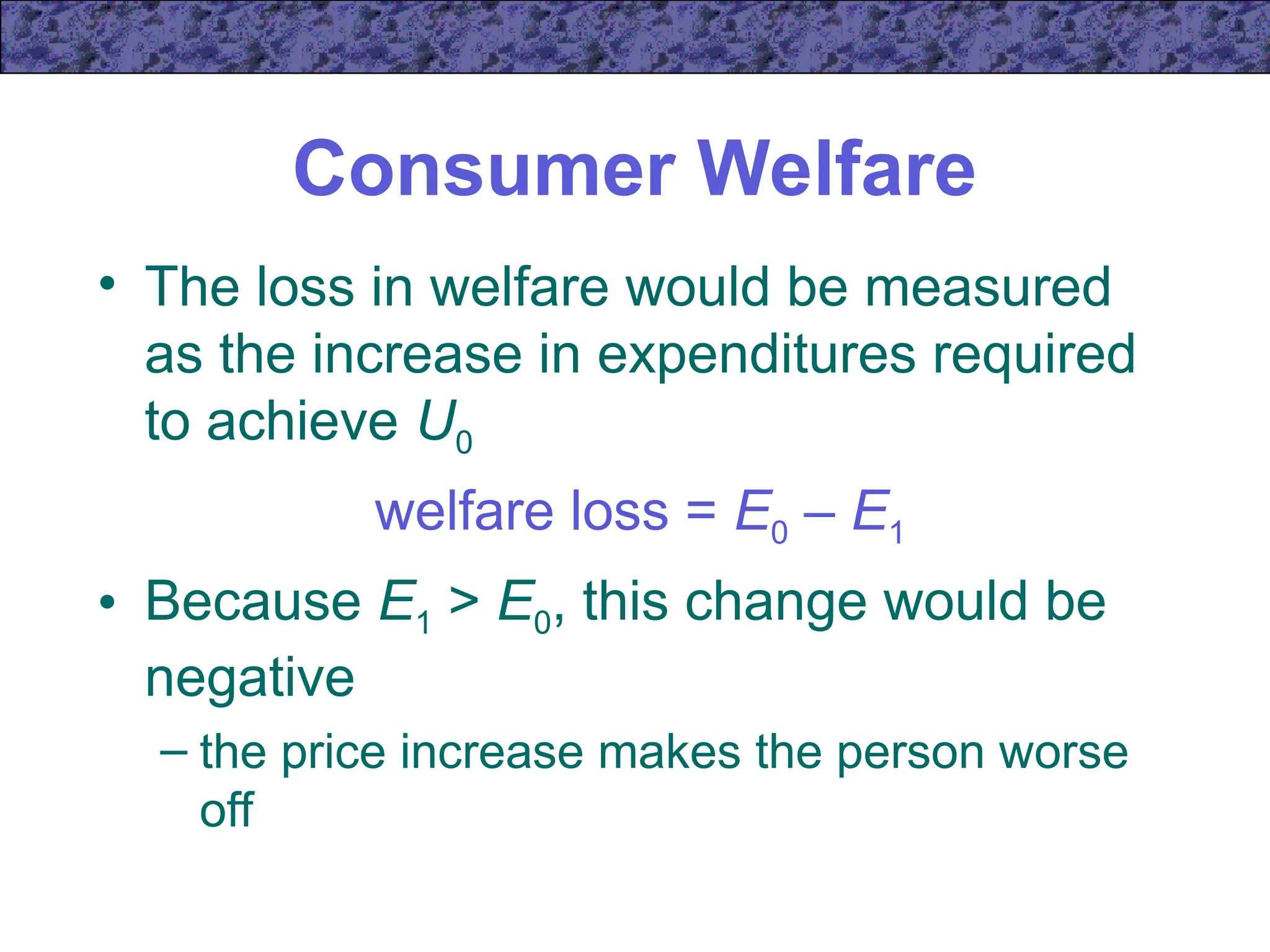
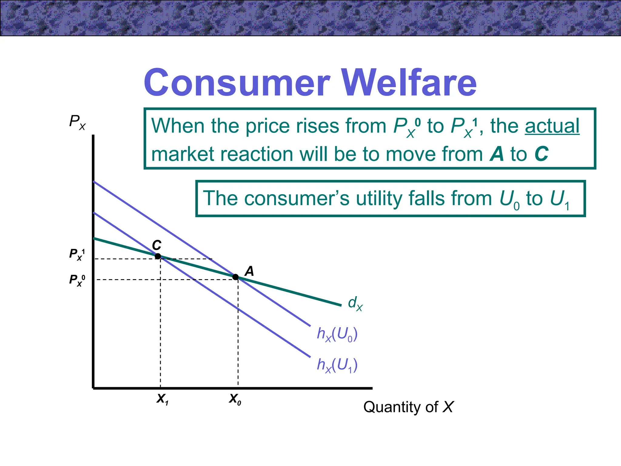
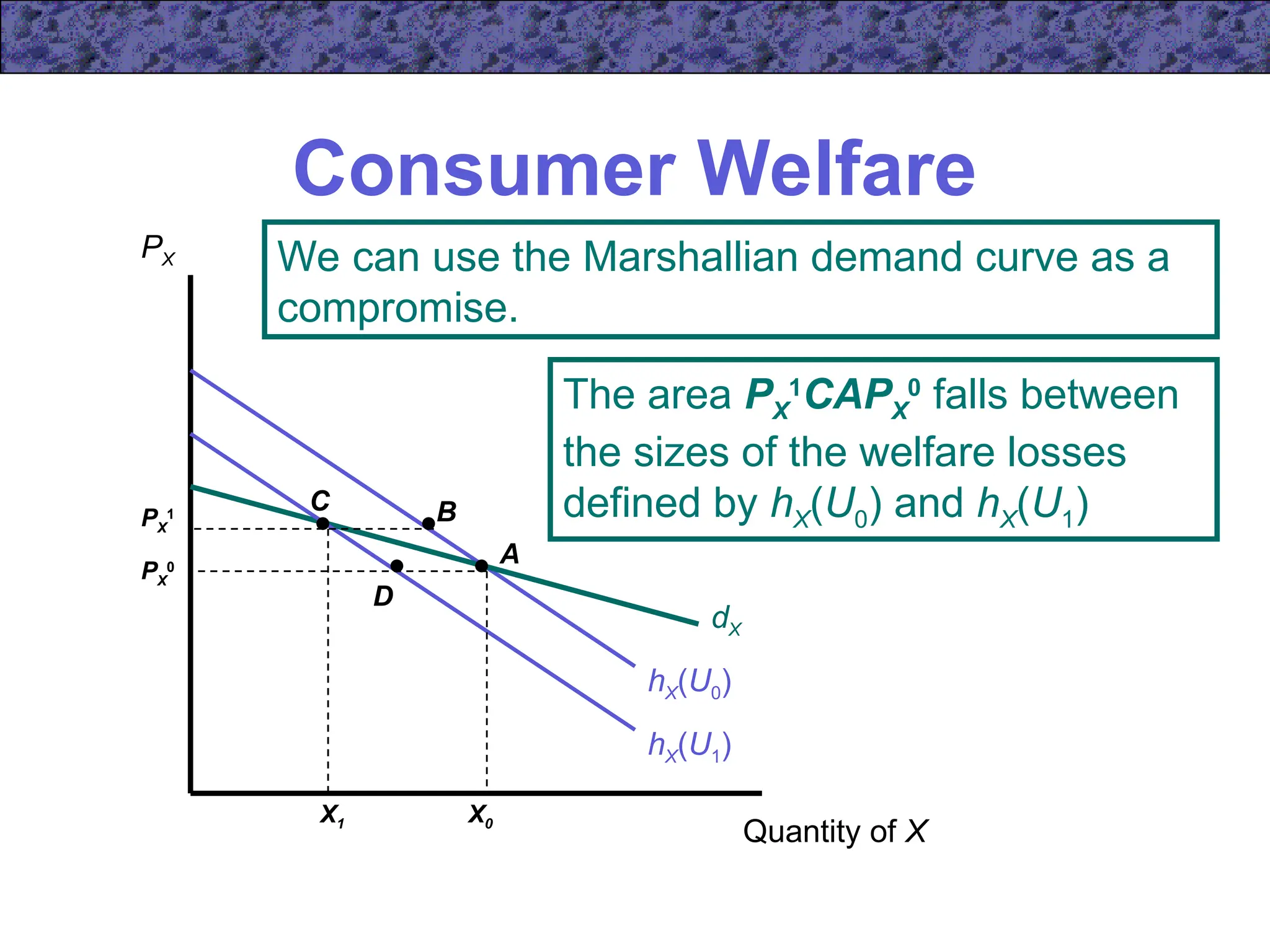
67. Consumer Welfare
Quantity of X
PX
hX(U0)
PX
1
X1
Is the consumer’s loss in welfare best
described by area PX
1
BAPX
0
[using hX(U0)]
or by area PX
1
CDPX
0
[using hX(U1)]?
hX(U1)
dX
A
B
C
D
PX
0
X0
Is U0 or U1 the appropriate
utility target?

68. Consumer Welfare
Quantity of X
PX
hX(U0)
PX
1
X1
We can use the Marshallian demand curve as a
compromise.
hX(U1)
dX
A
B
C
D
PX
0
X0
The area PX
1
CAPX
0
falls between
the sizes of the welfare losses
defined by hX(U0) and hX(U1)

69. Loss of Consumer Welfare
from a Rise in Price
• Suppose that the compensated demand
function for X is given by
5
0
5
0
.
.
)
,
,
(
X
Y
Y
X
X
P
VP
V
P
P
h
X 

the welfare loss from a price increase
from PX = 0.25 to PX = 1 is given by
1
25
0
5
0
5
0
1
25
0
5
0
5
0
2




X
X
P
P
X
Y
X
X
Y
P
VP
P
dP
VP
.
.
.
.
.
.

70. Loss of Consumer Welfare
from a Rise in Price
• If we assume that the initial utility level
(V) is equal to 2,
loss = 4(1)0.5
– 4(0.25)0.5
= 2
• If we assume that the utility level (V)
falls to 1 after the price increase (and
used this level to calculate welfare
loss),
loss = 2(1)0.5
– 2(0.25)0.5
= 1

71. Loss of Consumer Welfare
from a Rise in Price
• Suppose that we use the Marshallian
demand function instead
X
Y
X
X
P
P
P
d
X
2
I

 )
,
,
( I
the welfare loss from a price increase
from PX = 0.25 to PX = 1 is given by
1
25
0
1
25
0
2
2




X
X
P
P
X
X
X
P
dP
P .
.
ln
I
I

72. Loss of Consumer Welfare
from a Rise in Price
• Because income (I) is equal to 2,
loss = 0 – (-1.39) = 1.39
• This computed loss from the Marshallian
demand function is a compromise
between the two amounts computed
using the compensated demand
functions

73. Important Points to Note:
• Proportional changes in all prices and
income do not shift the individual’s budget
constraint and therefore do not alter the
quantities of goods chosen
– demand functions are homogeneous of degree
zero in all prices and income

74. Important Points to Note:
• When purchasing power changes (income
changes but prices remain the same),
budget constraints shift
– for normal goods, an increase in income
means that more is purchased
– for inferior goods, an increase in income
means that less is purchased

75. Important Points to Note:
• A fall in the price of a good causes
substitution and income effects
– For a normal good, both effects cause more of
the good to be purchased
– For inferior goods, substitution and income
effects work in opposite directions
• A rise in the price of a good also causes
income and substitution effects
– For normal goods, less will be demanded
– For inferior goods, the net result is ambiguous

76. Important Points to Note:
• The Marshallian demand curve summarizes
the total quantity of a good demanded at
each price
– changes in price prompt movemens along the
curve
– changes in income, prices of other goods, or
preferences may cause the demand curve to
shift

77. Important Points to Note:
• Compensated demand curves illustrate
movements along a given indifference
curve for alternative prices
– these are constructed by holding utility constant
– they exhibit only the substitution effects from a
price change
– their slope is unambiguously negative (or zero)

78. Important Points to Note:
• Income and substitution effects can be
analyzed using the Slutsky equation
• Income and substitution effects can also be
examined using revealed preference
• The welfare changes that accompany price
changes can sometimes be measured by
the changing area under the demand curve