1) The document presents a modified damped spring equation that is easier to tune and more stable than traditional springs. It derives the equation from first principles using the symplectic Euler integration method.
2) The modified equation sets stiffness and damping coefficients based on particle mass and timestep, eliminating the need to manually tune coefficients. It ensures the spring reaches equilibrium in one timestep, regardless of system parameters.
3) The equation is refactored to allow softness by introducing coefficients between 0-1. Setting coefficients to 1 yields rigid behavior, while lower values produce softer springs. The upper limits prevent instability from overshooting.
Strong Nuclear Force and Quantum Vacuum as Gravity (FUNDAMENTAL TENSOR)SergioPrezFelipe
Publication at ccsenet. Gravity explained by a new theory, ‘Superconducting String Theory (SST)’, completely opposite from current field emission based and inspired on originals string theories. Strengths are decomposed to make strings behave as one-dimensional structure with universe acting as a superconductor where resistance is near 0 and the matter moves inside. Strong nuclear force, with an attraction of 10.000 Newtons is which makes space to curve, generating acceleration, more matter more acceleration. Electromagnetic moves in 8 decimals, gravity is moved to more than 30 decimals to work as a superconductor.
Mechanical Vibrations Theory and Applications 1st Edition Kelly Solutions Manualvilyku
Full download http://alibabadownload.com/product/mechanical-vibrations-theory-and-applications-1st-edition-kelly-solutions-manual/
Mechanical Vibrations Theory and Applications 1st Edition Kelly Solutions Manual
Three Degree of Freedom Control of Inverted Pendulum by using Repulsive Magne...idescitation
An inverted pendulum is a pendulum which has its
mass above its pivot point. Inverted Pendulum is a classical
problem in dynamics and control theory and is widely used as
a benchmark for testing control algorithms (PID controllers,
neural networks, fuzzy control, genetic algorithms etc.).
Variations on this problem include multiple links allowing
the motion of the cart to be commanded while maintaining
the pendulum and balancing the cart- pendulum system on
see- saw. The inverted pendulum is related to rocket or missile
guidance, where the centre of gravity is located behind the
canter of drag causing aerodynamic instability. The
understanding of similar problem can be shown by balancing
an upturned broomstick on the end of one’s finger is a simple
demonstration and the problem is solved in the technology of
the seaway Position, self balancing transportation device. So,
here the entire above problem can be solved by using levitation
system. In this levitation system three magnets are used in
equilateral triangle for giving the force to inverted pendulum
in 3-dimension for balancing the pendulum.
Strong Nuclear Force and Quantum Vacuum as Gravity (FUNDAMENTAL TENSOR)SergioPrezFelipe
Publication at Publication at journal of advanced in physics. Gravity explained by a new theory, ‘Superconducting String Theory (SST)’, completely opposite from current field emission based and inspired on originals string theories. Strengths are decomposed to make strings behave as one-dimensional structure with universe acting as a superconductor where resistance is near 0 and the matter moves inside. Strong nuclear force, with an attraction of 10.000 Newtons is which makes space to curve, generating acceleration, more matter more acceleration. Electromagnetic moves in 8 decimals, gravity is moved to more than 30 decimals to work as a superconductor.
Learn Online Courses of Subject Engineering Mechanics of First Year Engineering. Clear the Concepts of Engineering Mechanics Through Video Lectures and PDF Notes. Visit us: https://ekeeda.com/streamdetails/subject/Engineering-Mechanics
De Alembert’s Principle and Generalized Force, a technical discourse on Class...Manmohan Dash
A technical discourse on formal classical mechanics. This is a 12 slide introduction to the basics of how Newton's Laws are generalized into a Lagrangian Dynamics apt at the level of an advance student of Physics.
12-1 EQUILIBRIUM\
After reading this module, you should be able to . . .
12.01 Distinguish between equilibrium and static equilibrium.
12.02 Specify the four conditions for static equilibrium.
12.03 Explain center of gravity and how it relates to center of
mass.
12.04 For a given distribution of particles, calculate the coordinates of the center of gravity and the center of mass.
12-2 SOME EXAMPLES OF STATIC EQUILIBRIUM
After reading this module, you should be able to . . .
12.05 Apply the force and torque conditions for static
equilibrium.
12.06 Identify that a wise choice about the placement of the origin (about which to calculate torques) can simplify the
calculations by eliminating one or more unknown forces
from the torque equation.
12-3 ELASTICITY
After reading this module, you should be able to . . .
12.07 Explain what an indeterminate situation is.
12.08 For tension and compression, apply the equation that
relates stress to strain and Young’s modulus.
12.09 Distinguish between yield strength and ultimate strength.
12.10 For shearing, apply the equation that relates stress to
strain and the shear modulus.
12.11 For hydraulic stress, apply the equation that relates
fluid pressure to strain and the bulk modulus. etc...
Strong Nuclear Force and Quantum Vacuum as Gravity (FUNDAMENTAL TENSOR)SergioPrezFelipe
Publication at ccsenet. Gravity explained by a new theory, ‘Superconducting String Theory (SST)’, completely opposite from current field emission based and inspired on originals string theories. Strengths are decomposed to make strings behave as one-dimensional structure with universe acting as a superconductor where resistance is near 0 and the matter moves inside. Strong nuclear force, with an attraction of 10.000 Newtons is which makes space to curve, generating acceleration, more matter more acceleration. Electromagnetic moves in 8 decimals, gravity is moved to more than 30 decimals to work as a superconductor.
Mechanical Vibrations Theory and Applications 1st Edition Kelly Solutions Manualvilyku
Full download http://alibabadownload.com/product/mechanical-vibrations-theory-and-applications-1st-edition-kelly-solutions-manual/
Mechanical Vibrations Theory and Applications 1st Edition Kelly Solutions Manual
Three Degree of Freedom Control of Inverted Pendulum by using Repulsive Magne...idescitation
An inverted pendulum is a pendulum which has its
mass above its pivot point. Inverted Pendulum is a classical
problem in dynamics and control theory and is widely used as
a benchmark for testing control algorithms (PID controllers,
neural networks, fuzzy control, genetic algorithms etc.).
Variations on this problem include multiple links allowing
the motion of the cart to be commanded while maintaining
the pendulum and balancing the cart- pendulum system on
see- saw. The inverted pendulum is related to rocket or missile
guidance, where the centre of gravity is located behind the
canter of drag causing aerodynamic instability. The
understanding of similar problem can be shown by balancing
an upturned broomstick on the end of one’s finger is a simple
demonstration and the problem is solved in the technology of
the seaway Position, self balancing transportation device. So,
here the entire above problem can be solved by using levitation
system. In this levitation system three magnets are used in
equilateral triangle for giving the force to inverted pendulum
in 3-dimension for balancing the pendulum.
Strong Nuclear Force and Quantum Vacuum as Gravity (FUNDAMENTAL TENSOR)SergioPrezFelipe
Publication at Publication at journal of advanced in physics. Gravity explained by a new theory, ‘Superconducting String Theory (SST)’, completely opposite from current field emission based and inspired on originals string theories. Strengths are decomposed to make strings behave as one-dimensional structure with universe acting as a superconductor where resistance is near 0 and the matter moves inside. Strong nuclear force, with an attraction of 10.000 Newtons is which makes space to curve, generating acceleration, more matter more acceleration. Electromagnetic moves in 8 decimals, gravity is moved to more than 30 decimals to work as a superconductor.
Learn Online Courses of Subject Engineering Mechanics of First Year Engineering. Clear the Concepts of Engineering Mechanics Through Video Lectures and PDF Notes. Visit us: https://ekeeda.com/streamdetails/subject/Engineering-Mechanics
De Alembert’s Principle and Generalized Force, a technical discourse on Class...Manmohan Dash
A technical discourse on formal classical mechanics. This is a 12 slide introduction to the basics of how Newton's Laws are generalized into a Lagrangian Dynamics apt at the level of an advance student of Physics.
12-1 EQUILIBRIUM\
After reading this module, you should be able to . . .
12.01 Distinguish between equilibrium and static equilibrium.
12.02 Specify the four conditions for static equilibrium.
12.03 Explain center of gravity and how it relates to center of
mass.
12.04 For a given distribution of particles, calculate the coordinates of the center of gravity and the center of mass.
12-2 SOME EXAMPLES OF STATIC EQUILIBRIUM
After reading this module, you should be able to . . .
12.05 Apply the force and torque conditions for static
equilibrium.
12.06 Identify that a wise choice about the placement of the origin (about which to calculate torques) can simplify the
calculations by eliminating one or more unknown forces
from the torque equation.
12-3 ELASTICITY
After reading this module, you should be able to . . .
12.07 Explain what an indeterminate situation is.
12.08 For tension and compression, apply the equation that
relates stress to strain and Young’s modulus.
12.09 Distinguish between yield strength and ultimate strength.
12.10 For shearing, apply the equation that relates stress to
strain and the shear modulus.
12.11 For hydraulic stress, apply the equation that relates
fluid pressure to strain and the bulk modulus. etc...
My name is Paulin O. I am associated with solidworksassignmenthelp.com for the past 10 years and have been helping the engineering students with their assignments I have a Masters in mechanical Engineering from Cornell University, USA.
Iterative constraint solvers work great, but there are cases where we could use better convergence. This presentation explores various Mixed Linear Complementarity Problem (MLCP) solvers and the Featherstone articulated body algorithm and how to mix them.
Structural Analysis Report
If you are a beginner for Ansys must watch this video (https://youtu.be/eAf2eBYY6GU) basic to advance.
In this video, we will perform structural analysis.With the help of Ansys Fea Software.This is a fantastic video for beginners as well as for a skilled one because I have covered all concepts is a beautiful manner
There are many Finite element analysis software available in the market but ANSYS is one of the best simulation software you can download it at Ansys company website which is free for students.For simulation services please contact me
I can solve FEA problems is an economical price
contact me;
515mrigendra@gmail.com
Study of a Gear-Rack and links System: Equations, configuration and CAD designPietro Galli
The study dealt with the Designing of a mechanism form a starting configuration. Development of equations (Study of the motion and of the velocities), CAD files and engineer drawings (Using Solidworks)
REPORT SUMMARYVibration refers to a mechanical.docxdebishakespeare
REPORT SUMMARY
Vibration refers to a mechanical phenomenon involving oscillations about a point. These oscillations can be of any imaginable range of amplitudes and frequencies, with each combination having its own effect. These effects can be positive and purposefully induced, but they can also be unintentional and catastrophic. It's therefore imperative to understand how to classify and model vibration.
Within the classroom portion of ME 345, we discussed damped and undamped vibrations, appropriate models, and several of their properties. The purpose of Lab 3 is to give us the corresponding "hands-on" experience to cement our understanding of the theory.
As it turns out, vibration can be modeled with a simple spring-mass system (spring-mass-damper system for damped vibration). In order to create a mathematical model for our simple spring-mass system, we apply Newton's second law and sum the forces about the mass. After applying some of our knowledge of differential equations, the result is a second order linear differential equation (in vector form). This can easily be converted to the scalar version, from which it's easy to glean various properties of the vibration (i.e. natural frequency, period, etc.).
In the lab, we were provided with a PASCO motion sensor, USB link, ramp, and accompanying software. All of the aforementioned equipment was already assembled and connected. The ramp was set up at an angle with a stop on the elevated end and the motion sensor on the lower end. The sensor was connected to the USB link, which was in turn connected to the computer. We chose to use the Xplorer GLX software to interface with the sensor and record our data. After receiving our equipment, we gathered data on our spring's extension with a known load to derive a spring constant. We were provided with a small cart to which we attached weights to increase its mass. In order to model free vibration, we placed the cart on the track and attached it to the stop at the top of the ramp with a spring. After displacing the cart a certain distance from its equilibrium point, the cart was released and was allowed to oscillate on the track while we recorded its distance from the sensor. This was done with displacements of -20cm, -10cm, +10cm, and +20cm from the system's equilibrium point. After gathering this data for the "free" case, a magnet was attached to the front of the car, spaced as far from the track as possible. As the track is magnetic, this caused a slight damping effect, basically converting our spring-mass system to an underdamped spring-mass-damper system. After repeating the procedure for the "free" case, we moved the magnets as close to the track as possible (causing the system to become overdamped) and again repeated the procedure for the "free" case.
We were finally able to determine the period, phase angle, damping coefficients, and circular and cyclical frequencies for the three systems. There were similarities and differ ...
EGME 431 Term ProjectJake Bailey, CSU FullertonSpring .docxSALU18
EGME 431 Term Project
Jake Bailey, CSU Fullerton
Spring 2016
This document serves to set forth the requirements for your term project, and the criteria
which such project submissions shall be judged. This outline should be the first point of inquiry
for any questions you may have about your project.
The project consists of a thorough investigation, analysis, and set of design improvement sug-
gestions for a simplified automobile suspension model. The dynamics of this model are rather
complex: as such, I have provided a detailed derivation of the equations of motion for this system
to you in a separate document. Your responsibility will be that of the analyst: use the provided dy-
namic models to investigate the system’s response to typical inputs, judge these responses critically,
and suggest improvements to the system.
Your project submissions shall consist of a single analysis and design report. The project
report shall be turned in no later than the final class meeting of the semester, which is May 10,
2016 at 7:00 PM. As always, late assignments will not be accepted. The report shall, at a minimum,
include:
• A description of your analysis methodology
• A summary of the important results from your analyses, including plots and data tables where
appropriate
• A thorough defense of your analysis results, including (but not limited to):
– comparison with analytical approximations
– investigation of typical results of published investigations, and
– discussion and investigation of the approximate errors accrued in your simulations
• A succinct description of the modifications you propose to improve the performance of the
system, including justification of your choices
The dynamic models which have been provided to you include both a fully coupled, non-linear
model and a simplified, linearized version. It is up to you to decide which to use for each portion
of the tasks outlined below. Note, however, that you should, at a minimum, simulate both models
under a common input. This will server as a basis for comparison.
Your specific tasks for this project are as follows:
1. Find the response of the system to a variety of inputs, including steps, impulses, and harmonic
excitation.
2. Determine the Displacement Transmissibility Ratio and Force Transmissibility Ratio of the
system over a range of input frequencies.
1
3. Using judgment, analytical techniques, and/or optimization methods, find a new set of sys-
tem parameters (stiffnesses and damping coefficients) which will improve the response of the
system to the selected inputs.
4. Finally, prepare a report which thoroughly summarizes and defends your methodology and
results.
A final word on collaboration. You are encouraged to discuss your ideas and your solution
approach with your classmates and colleagues. You are, however, expressly forbidden from sharing
simulation data, code, spreadsheets, scripts, or the like with anyone. Two students submitting
substantially similar s ...
Lab 05 – Gravitation and Keplers Laws Name __________________.docxDIPESH30
Lab 05 – Gravitation and Keplers Laws Name: _____________________
Why everyone in this class is attracted to everyone else.
https://phet.colorado.edu/en/simulation/gravity-force-lab
Adapted from Chris Bier’s Collisions PhET Lab OPTION A: CREATIVE COMMONS - ATTRIBUTION
Introduction:
Every object around you is attracted to you. In fact, every object in the galaxy is attracted to every other object in the galaxy. Newton postulated and Cavendish confirmed that all objects with mass are attracted to all other objects with mass by a force that is proportional to their masses and inversely proportional to the square of the distance between the objects' centers. This relationship became Newton's Law of Universal Gravitation. In this simulation, you will look at two massive objects and their gravitational force between them to observe G, the constant of universal gravity that Cavendish investigated.
Important Formulas:
Procedure: https://phet.colorado.edu/en/simulation/gravity-force-lab
1. Take some time and familiarize yourself with the simulation. Notice how forces change as mass changes and as distance changes.
2. Fill out the chart below for the two objects at various distances.
3. Rearranging the equation for Force, you can CALCULATE the value of G using the values given below for m1, m2, and d, and the value for the Force that you obtain in the simulation. Record the force between the two object and then solve (calculate G) for the universal gravitation constant, G and compare it to values published in books, online, or your text book. The numbers you calculate for G will vary slightly from row to row. Remember significant digits!15 pts
Mass Object 1 Mass Object 2 Distance Force Gravitation Constant,G
50.00 kg
25.00 kg
3.0m
50.00 kg
25.00 kg
4.0m
50.00 kg
25.00 kg
5.0m
50.00 kg
25.00 kg
6.0m
50.00 kg
25.00 kg
9.0m
What do you notice about the force that acts on each object? 3 pts
[Answer Here]
Average value of G: _________________2 ptsUnits of G: _______________2 pts
Published value of G: ________________2 pts Source: _______________2 pts
How did your average value of G compare to the published value for G that you found? 3 pts
[Answer Here]
Conclusion Questions and Calculations:Bold and Underlinethe correct answer to each question.
1. Gravitational force is always attractive / repulsive. (circle) 2 pts
2. Newton’s 3rd Law tells us that if a gravitational force exists between two objects, one very massive and one less massive, then the force on the less massive object will be greater than / equal to / less than the force on the more massive object. 2 pts
3. The distance between masses is measured from their edges between them / from their centers / from the edge of one to the center of the other. 2 pts
4. As the distance between masses decreases, force increases / decreases. 2 pts
5. Doubling the mass of both masses would result in a change of force between the mas ...
UiPath Test Automation using UiPath Test Suite series, part 4DianaGray10
Welcome to UiPath Test Automation using UiPath Test Suite series part 4. In this session, we will cover Test Manager overview along with SAP heatmap.
The UiPath Test Manager overview with SAP heatmap webinar offers a concise yet comprehensive exploration of the role of a Test Manager within SAP environments, coupled with the utilization of heatmaps for effective testing strategies.
Participants will gain insights into the responsibilities, challenges, and best practices associated with test management in SAP projects. Additionally, the webinar delves into the significance of heatmaps as a visual aid for identifying testing priorities, areas of risk, and resource allocation within SAP landscapes. Through this session, attendees can expect to enhance their understanding of test management principles while learning practical approaches to optimize testing processes in SAP environments using heatmap visualization techniques
What will you get from this session?
1. Insights into SAP testing best practices
2. Heatmap utilization for testing
3. Optimization of testing processes
4. Demo
Topics covered:
Execution from the test manager
Orchestrator execution result
Defect reporting
SAP heatmap example with demo
Speaker:
Deepak Rai, Automation Practice Lead, Boundaryless Group and UiPath MVP
Elevating Tactical DDD Patterns Through Object CalisthenicsDorra BARTAGUIZ
After immersing yourself in the blue book and its red counterpart, attending DDD-focused conferences, and applying tactical patterns, you're left with a crucial question: How do I ensure my design is effective? Tactical patterns within Domain-Driven Design (DDD) serve as guiding principles for creating clear and manageable domain models. However, achieving success with these patterns requires additional guidance. Interestingly, we've observed that a set of constraints initially designed for training purposes remarkably aligns with effective pattern implementation, offering a more ‘mechanical’ approach. Let's explore together how Object Calisthenics can elevate the design of your tactical DDD patterns, offering concrete help for those venturing into DDD for the first time!
GDG Cloud Southlake #33: Boule & Rebala: Effective AppSec in SDLC using Deplo...James Anderson
Effective Application Security in Software Delivery lifecycle using Deployment Firewall and DBOM
The modern software delivery process (or the CI/CD process) includes many tools, distributed teams, open-source code, and cloud platforms. Constant focus on speed to release software to market, along with the traditional slow and manual security checks has caused gaps in continuous security as an important piece in the software supply chain. Today organizations feel more susceptible to external and internal cyber threats due to the vast attack surface in their applications supply chain and the lack of end-to-end governance and risk management.
The software team must secure its software delivery process to avoid vulnerability and security breaches. This needs to be achieved with existing tool chains and without extensive rework of the delivery processes. This talk will present strategies and techniques for providing visibility into the true risk of the existing vulnerabilities, preventing the introduction of security issues in the software, resolving vulnerabilities in production environments quickly, and capturing the deployment bill of materials (DBOM).
Speakers:
Bob Boule
Robert Boule is a technology enthusiast with PASSION for technology and making things work along with a knack for helping others understand how things work. He comes with around 20 years of solution engineering experience in application security, software continuous delivery, and SaaS platforms. He is known for his dynamic presentations in CI/CD and application security integrated in software delivery lifecycle.
Gopinath Rebala
Gopinath Rebala is the CTO of OpsMx, where he has overall responsibility for the machine learning and data processing architectures for Secure Software Delivery. Gopi also has a strong connection with our customers, leading design and architecture for strategic implementations. Gopi is a frequent speaker and well-known leader in continuous delivery and integrating security into software delivery.
JMeter webinar - integration with InfluxDB and GrafanaRTTS
Watch this recorded webinar about real-time monitoring of application performance. See how to integrate Apache JMeter, the open-source leader in performance testing, with InfluxDB, the open-source time-series database, and Grafana, the open-source analytics and visualization application.
In this webinar, we will review the benefits of leveraging InfluxDB and Grafana when executing load tests and demonstrate how these tools are used to visualize performance metrics.
Length: 30 minutes
Session Overview
-------------------------------------------
During this webinar, we will cover the following topics while demonstrating the integrations of JMeter, InfluxDB and Grafana:
- What out-of-the-box solutions are available for real-time monitoring JMeter tests?
- What are the benefits of integrating InfluxDB and Grafana into the load testing stack?
- Which features are provided by Grafana?
- Demonstration of InfluxDB and Grafana using a practice web application
To view the webinar recording, go to:
https://www.rttsweb.com/jmeter-integration-webinar
Transcript: Selling digital books in 2024: Insights from industry leaders - T...BookNet Canada
The publishing industry has been selling digital audiobooks and ebooks for over a decade and has found its groove. What’s changed? What has stayed the same? Where do we go from here? Join a group of leading sales peers from across the industry for a conversation about the lessons learned since the popularization of digital books, best practices, digital book supply chain management, and more.
Link to video recording: https://bnctechforum.ca/sessions/selling-digital-books-in-2024-insights-from-industry-leaders/
Presented by BookNet Canada on May 28, 2024, with support from the Department of Canadian Heritage.
Essentials of Automations: Optimizing FME Workflows with ParametersSafe Software
Are you looking to streamline your workflows and boost your projects’ efficiency? Do you find yourself searching for ways to add flexibility and control over your FME workflows? If so, you’re in the right place.
Join us for an insightful dive into the world of FME parameters, a critical element in optimizing workflow efficiency. This webinar marks the beginning of our three-part “Essentials of Automation” series. This first webinar is designed to equip you with the knowledge and skills to utilize parameters effectively: enhancing the flexibility, maintainability, and user control of your FME projects.
Here’s what you’ll gain:
- Essentials of FME Parameters: Understand the pivotal role of parameters, including Reader/Writer, Transformer, User, and FME Flow categories. Discover how they are the key to unlocking automation and optimization within your workflows.
- Practical Applications in FME Form: Delve into key user parameter types including choice, connections, and file URLs. Allow users to control how a workflow runs, making your workflows more reusable. Learn to import values and deliver the best user experience for your workflows while enhancing accuracy.
- Optimization Strategies in FME Flow: Explore the creation and strategic deployment of parameters in FME Flow, including the use of deployment and geometry parameters, to maximize workflow efficiency.
- Pro Tips for Success: Gain insights on parameterizing connections and leveraging new features like Conditional Visibility for clarity and simplicity.
We’ll wrap up with a glimpse into future webinars, followed by a Q&A session to address your specific questions surrounding this topic.
Don’t miss this opportunity to elevate your FME expertise and drive your projects to new heights of efficiency.
Accelerate your Kubernetes clusters with Varnish CachingThijs Feryn
A presentation about the usage and availability of Varnish on Kubernetes. This talk explores the capabilities of Varnish caching and shows how to use the Varnish Helm chart to deploy it to Kubernetes.
This presentation was delivered at K8SUG Singapore. See https://feryn.eu/presentations/accelerate-your-kubernetes-clusters-with-varnish-caching-k8sug-singapore-28-2024 for more details.
Software Delivery At the Speed of AI: Inflectra Invests In AI-Powered QualityInflectra
In this insightful webinar, Inflectra explores how artificial intelligence (AI) is transforming software development and testing. Discover how AI-powered tools are revolutionizing every stage of the software development lifecycle (SDLC), from design and prototyping to testing, deployment, and monitoring.
Learn about:
• The Future of Testing: How AI is shifting testing towards verification, analysis, and higher-level skills, while reducing repetitive tasks.
• Test Automation: How AI-powered test case generation, optimization, and self-healing tests are making testing more efficient and effective.
• Visual Testing: Explore the emerging capabilities of AI in visual testing and how it's set to revolutionize UI verification.
• Inflectra's AI Solutions: See demonstrations of Inflectra's cutting-edge AI tools like the ChatGPT plugin and Azure Open AI platform, designed to streamline your testing process.
Whether you're a developer, tester, or QA professional, this webinar will give you valuable insights into how AI is shaping the future of software delivery.
Dev Dives: Train smarter, not harder – active learning and UiPath LLMs for do...UiPathCommunity
💥 Speed, accuracy, and scaling – discover the superpowers of GenAI in action with UiPath Document Understanding and Communications Mining™:
See how to accelerate model training and optimize model performance with active learning
Learn about the latest enhancements to out-of-the-box document processing – with little to no training required
Get an exclusive demo of the new family of UiPath LLMs – GenAI models specialized for processing different types of documents and messages
This is a hands-on session specifically designed for automation developers and AI enthusiasts seeking to enhance their knowledge in leveraging the latest intelligent document processing capabilities offered by UiPath.
Speakers:
👨🏫 Andras Palfi, Senior Product Manager, UiPath
👩🏫 Lenka Dulovicova, Product Program Manager, UiPath
Slack (or Teams) Automation for Bonterra Impact Management (fka Social Soluti...Jeffrey Haguewood
Sidekick Solutions uses Bonterra Impact Management (fka Social Solutions Apricot) and automation solutions to integrate data for business workflows.
We believe integration and automation are essential to user experience and the promise of efficient work through technology. Automation is the critical ingredient to realizing that full vision. We develop integration products and services for Bonterra Case Management software to support the deployment of automations for a variety of use cases.
This video focuses on the notifications, alerts, and approval requests using Slack for Bonterra Impact Management. The solutions covered in this webinar can also be deployed for Microsoft Teams.
Interested in deploying notification automations for Bonterra Impact Management? Contact us at sales@sidekicksolutionsllc.com to discuss next steps.
Encryption in Microsoft 365 - ExpertsLive Netherlands 2024Albert Hoitingh
In this session I delve into the encryption technology used in Microsoft 365 and Microsoft Purview. Including the concepts of Customer Key and Double Key Encryption.
Encryption in Microsoft 365 - ExpertsLive Netherlands 2024
Hatten spring 1561232600_stablesprings0.7.3
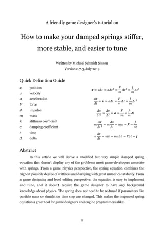
1. 1
A friendly game designer's tutorial on
How to make your damped springs stiffer,
more stable, and easier to tune
Written by Michael Schmidt Nissen
Version 0.7.3, July 2019
Quick Definition Guide
x position
v velocity
a acceleration
F force
J impulse
m mass
k stiffness coefficient
c damping coefficient
t time
Δ delta
Abstract
In this article we will derive a modified but very simple damped spring
equation that doesn't display any of the problems most game-developers associate
with springs. From a game physics perspective, the spring equation combines the
highest possible degree of stiffness and damping with great numerical stability. From
a game designing and level editing perspective, the equation is easy to implement
and tune, and it doesn't require the game designer to have any background
knowledge about physics. The spring does not need to be re-tuned if parameters like
particle mass or simulation time step are changed. This makes the improved spring
equation a great tool for game designers and engine programmers alike.
2. 2
The trouble with springs...
In the game development community, the damped spring based on Hooke's
law of elasticity is often regarded as the black sheep of game physics, and a number
of notable books, papers and websites warns the reader against implementing them.
There are at least two good reasons for this.
The most straight-forward reason is that springs are notoriously difficult to
tune. It can be very time consuming to adjust the stiffness and damping coefficients
in order to make a simulation behave just right. For large spring systems the task can
be daunting. If a single variable is changed, for instance a spring coefficient, the mass
of a particle, or the physics engine time step, you might have to re-tune everything
from scratch.
A deeper reason for avoiding springs is that they are prone to instability. Every
once in a while, a system of connected springs and particles will blow up in your face
without warning, and for no apparent reason – usually followed by a program crash.
This happens because either simulation time step or spring coefficients have been set
too high, or particle mass has been set too low, placing the simulation outside it's
(usually unknown) range of stability.
The problem is that there’s no simple or death-proof way to determine what
combination of values adds up to a stable system. Thus, the game designer's ability to
balance a spring system often relies on experience and “gut feeling”, which makes it
look more like black magic than actual physics. This lack of transparency is why the
game development community looks upon springs with a lot of suspicion.
Improving Hooke's infamous damped spring
In the following pages we will do a complete breakdown of the math behind
damped springs and use it to reformulate the old equation in a way that makes sense
for game developers. We will only be focusing on how springs work in the discrete
time-stepping world of game physics, not how they work in real-life, which is a
slightly different thing. First, let's take a look at the equation at hand:
The equation is divided up into two parts. The first part calculates a spring
3. 3
force that is linearly proportional to displacement x, and the second part calculates a
damping force that is linearly proportional to velocity v. The value of the stiffness
and damping coefficients k and c decide the magnitude of the forces.
Game designers usually want a spring to be as rigid as possible. That is, they
want it to behave like a steel rod, and not like a soggy old rubber band. But what k
and c values do we plug in to achieve this behaviour? 0.001? 1.337E42? For someone
who doesn't understand the underlying math it is basically trial-and-error: Plug in a
random value. If the spring behaves too sloppy, increase the value, and if the
simulation becomes jittery or explodes, decrease it.
In the following section we will derive a spring equation that eliminates this
challenge and allows the game designer to implement a spring that will always stay
inside the safe region of stability and will reach its rest state in as little as one loop.
To explain how this is done we first need to take a look at our integrator – the part of
the program that computes new particle velocities and positions based on the forces
applied to them. The most commonly used integrator is the so-called symplectic
Euler or semi-explicit Euler method:
This integrator is popular because it is very easy to implement, and it displays
great energy conservation and stability compared to similar algorithms. Please notice
that velocity is expressed as v = a Δt, and that distance is expressed as x = v Δt.
Let's move on and look at a damped spring attached to a fixed point in one end
and a particle in the other. Assume that the particle is displaced distance x from its
rest position. Now let us try to find the force required to move it the opposite
distance in one loop with the symplectic Euler algorithm. From Newton's 2nd law of
motion we know that a = F / m, which give us the following relationship between
distance and force:
4. 4
The minus sign simply means that we are going in the opposite direction of the
displacement. Now we can isolate force:
And since the spring force in Hooke's law of elasticity is defined as:
It becomes immediately clear that:
Which is the exact stiffness coefficient value required to move the particle
back to its rest position in one simulation loop. However, since we are not doing
anything to stop the particle, it will keep oscillating back and forth through the rest
position. We need to add damping, which is done with the second part of the spring
equation.
Let's assume the particle has a velocity v that we want to eliminate. By
calculating the amount of force needed to exactly counter this velocity, we can make
the particle stop at the rest distance. In the Symplectic Euler integration algorithm
we have the following relationship between velocity and force:
When isolating force we get:
5. 5
And since the damping force is defined:
We immediately see by inspection that the damping coefficient is:
This is the exact damping coefficient value needed to make the spring stop the
particle in one simulation loop. Now we can join the two parts and write out the
complete damped spring equation in its most raw and basic form:
This spring equation has some very interesting properties. The first thing we
notice is the lack of coefficients. We've simply replaced k with m/Δt2 and c with m/Δt.
When implementing the equation we see that it really does work! The spring reaches
rest length and stops dead without any oscillation in one loop, completely
independent of particle position, velocity, mass, and physics engine time step.
This is the stiffest possible spring we can imagine, and it displays behaviour
more similar to a rigid constraint than a soft, bouncy spring. We have found the steel
rod spring we were looking for in the beginning of the chapter. The equation also has
another interesting property. It simply cannot blow up no matter what values we
throw at it. Practically speaking, we can regard the spring as being unconditionally
stable.
We can refactor the equation a bit so it's easier to use in a programming
context. Now time step, state, and mass are separated, which makes it easier to write
re-useable code. Since physics engines normally run with a fixed time step, we can
also pre-compute the 1/Δt and 1/Δt2
values and save a few precious CPU-cycles.
6. 6
Re-introducing coefficients
Now we have a really powerful spring equation. It is easy to implement, very
stable, and it reaches its rest-state in just one loop. But in our quest towards a better
spring it has lost its springiness. We need to get the softness and bounciness back
again, and for this purpose we will re-introduce stiffness and damping coefficients.
To avoid confusion, the new coefficients are named Cs and Cd. While the
original coefficients could represent any positive numerical value, these both lie in
the interval between zero and one.
As we can see, the new coefficients are simply the fraction of completely rigid
behaviour we would like the spring to display. Soft, bouncy springs would usually
have values in the range of 0.00001 – 0.001. In the other end of the scale, values of
just 0.01 – 0.1 is enough to display rigid behaviour. Setting both values to 1.0 would
of course still satisfy the spring in one loop.
Please notice that spring behaviour is determined exclusively by these two
coefficients. Particle mass or simulation time step has literally no influence on how
the spring behaves, and changing them – even during runtime – wouldn't make it
necessary to re-tune the system. This makes the spring a much more powerful and
developer-friendly tool that can be used safely by designers without any worries
about possible future changes in game physics.
Interestingly, the spring will get less rigid and less stable if we increase the Cs
or Cd values above one. This happens because the particles overshoot their target rest
values, leading to undefined behaviour. If we keep increasing either or both of the
coefficients, the system will start to jitter, and at some point it will ride the Neptune
Express. In other words, we have – almost by accident – determined the exact upper
limit for the two spring coefficients, which we can define:
This also allows us to simplify the spring a bit, making it almost as simple as
7. 7
the equation we started out with:
Now it also becomes clear why so many people dislike the Hooke's law spring
equation. Not because it is inherently bad, but because it is so easy to accidentally
plug in a coefficient value that doesn't make any sense. The equation derived in this
paper always scales spring force to fit time step and mass, but the original equation
does not.
This makes it very easy for the less physics-minded game designer to
inadvertently plug in a coefficient value above the upper limits we have just derived.
In the original equation it isn't even apparent that there is such a thing as an upper
limit. I would like to stress the point that this lack of transparency in the original
Hooke's law spring is the main reason why so many people have frustrating
experiences with it.
Two connected particles with different mass
It is only slightly more complicated to constrain two free-moving particles
with the improved spring. To do this, we need to introduce the concept of reduced
mass. This is a quantity that can be used to compute interactions between two bodies
as-if one body were stationary, which allows us to reuse the equation we've already
derived. The reduced mass for two particles with mass ma and mb is defined:
Since the inverse mass quantity is often pre-computed for other purposes, it can also
be useful to define reduced mass like this:
Unsurprisingly, the maximum coefficient values for two connected particles are:
8. 8
Which gives us the following equation to work with:
This spring equation will move two connected particles of any given mass to
rest distance and make them stand still relative to each other in one loop. However,
since angular momentum is conserved, the particles may rotate around each other,
which will make the bodies come to rest at a larger distance, depending on how fast
they spin.
Impulse-based spring
Today, most physics engines are based on impulses, or direct changes in
velocities, rather than forces and acceleration. The spring equation described above
works just as well if we redesign it to work at impulse-level. Since impulse is defined
J = F Δt, the symplectic Euler integration algorithm needs a little update:
The maximum coefficient values for the impulse based spring are:
This gives us the following impulse based spring to work with. When used
with the integration algorithm shown above, this equation returns the numerically
exact same result as the force based spring we derived earlier in the paper.
9. 9
And that pretty much sums it up. Now I think it's about time we got our hands dirty
and turned all the math into a working piece of code.
From math to code
I am using C++ syntax in the following code snippets, but for the sake of
brevity and clarity I have kept them unoptimized and as simple as possible. With a
little effort you should be able to make them run in your own favourite programming
language. First let's define the particle class, which should be pretty self-explanatory:
class Particle
{
vec2 position; //
vec2 velocity; //
vec2 impulse; //
float inverse_mass; // Set to zero for infinite mass = static object.
};
Next we have the spring class, which is equally simple:
class Spring
{
vec2 unit_vector; // Normalized distance vector.
float rest_distance; //
float reduced_mass; //
Particle* particle_a; // Pointer to endpoint particle a.
Particle* particle_b; // Pointer to endpoint particle b.
};
Then we have the function that updates particle state. This part of the code
implements the symplectic Euler integration algorithm and it is important to
understand that the spring equation is tailored to be used with this update method. If
you swap this out with another algorithm, it will probably break the logic of the
spring equation.
10. 10
void ComputeNewState( Particle* P )
{
// Compute new velocity from impulse, scaled by mass.
P->velocity += P->impulse * P->inverse_mass;
// Compute new position from velocity.
P->position += P->velocity * TIMESTEP;
// Reset impulse vector.
P->impulse = Vec2( 0.0, 0.0 );
}
Finally there is the function that computes and applies the spring impulse to
its two endpoint particles. This is the core of our physics engine, and this is where the
spring equation dwells.
void ComputeSpringImpulse( Spring* S )
{
// First we calculate the distance and velocity vectors.
vec2 distance = S->particle_b->position - S->particle_a->position;
vec2 velocity = S->particle_b->velocity - S->particle_a->velocity;
// We normalize the distance vector to get the unit vector.
S->unit_vector = distance.normalize();
// Now we calculate the distance and velocity errors.
float distance_error = S->unit_vector.dot( distance ) - S->rest_distance;
float velocity_error = S->unit_vector.dot( velocity );
// Now we use the spring equation to calculate the impulse.
float distance_impulse = C_S * distance_error * INVERSE_TIMESTEP;
float velocity_impulse = C_D * velocity_error;
float impulse = -( distance_impulse + velocity_impulse ) * S->reduced_mass;
// Finally, we apply opposite equal impulses to the endpoint particles.
S->particle_a->impulse -= impulse * S->unit_vector;
S->particle_b->impulse += impulse * S->unit_vector;
}
11. 11
Limitations and Pitfalls
When connecting multiple springs and particles into larger bodies, we run into
the same trouble as with any other type of constraint. Rather than cooperating, they
tend to compete against each other, and this spells trouble. When a spring moves two
particles to satisfy distance and velocity, it usually means dissatisfying one or several
other springs. It is outside the scope of this article to dig deeply into this problem,
but I would like to provide a bit of advice on how to prevent the worst disasters.
When two or more springs are connected to the same particle, which is the
case in any kind of rope, mesh, or squishy body, setting the coefficients to the
maximum value of 1.0 will lead to stability problems. Although the spring equation is
stable when particles are connected to just one spring, this is sadly not the case for
higher number of springs. After some lengthy tampering I have worked out that a
safe upper limit for both the stiffness and damping coefficient is:
Where n denotes the highest number of springs attached to any of the two
particles connected by the spring. So for example, in a rope where any particle is
connected by at most two springs, Cs and Cd can both safely be set to 0.33, and in a
square mesh, where any particle is at most connected by four springs, they can be set
to 0.2.
Conclusion and future work
As promised, I have managed to derive a very stable, rigid, and user-friendly
spring equation over the course of a few pages. The math behind the equation is
surprisingly simple, which makes me wonder why it hasn't been described or
implemented decades ago. In the next article, we will look further into the mentioned
limitations when implementing large systems of interconnected springs and improve
it even further using an iterative approach with warm starting.
12. 12
About the author
Michael Schmidt Nissen lives in Denmark and currently makes a living as a
historical blacksmith. He extracts iron and steel from local ores using the same
techniques as his Viking ancestors. Programming, especially small games and
physics simulations, has been a beloved hobby ever since Michael learned to code in
the golden era of the Commodore 64 and Amiga 500.
If you enjoyed reading this article, please consider giving it some constructive
feedback and share it with your colleagues. Also, if you use the spring equation in a
game or demo, please give the author credit for it.
Links
https://en.wikipedia.org/wiki/Hooke%27s_law
https://en.wikipedia.org/wiki/Newton%27s_laws_of_motion
https://en.wikipedia.org/wiki/Reduced_mass
https://en.wikipedia.org/wiki/Semi-implicit_Euler_method
http://gafferongames.com/game-physics/spring-physics/