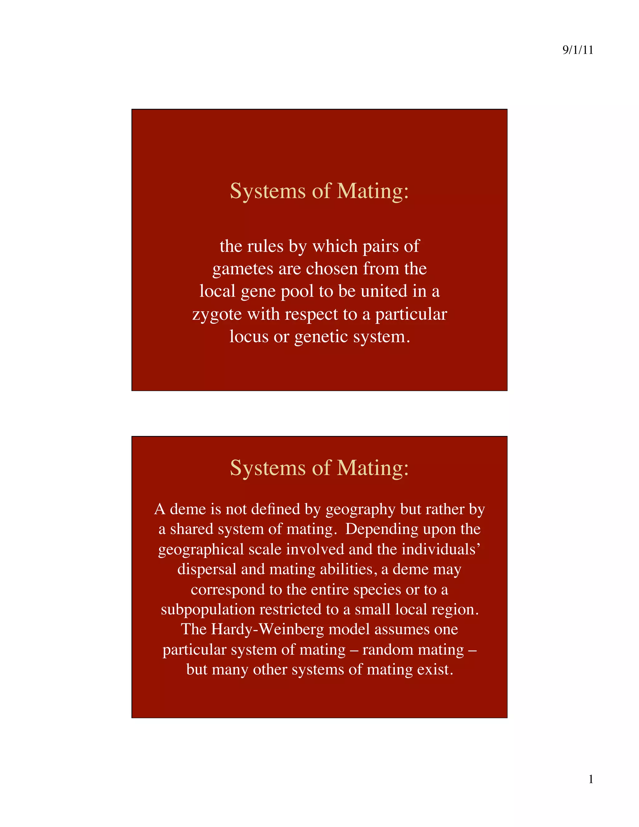
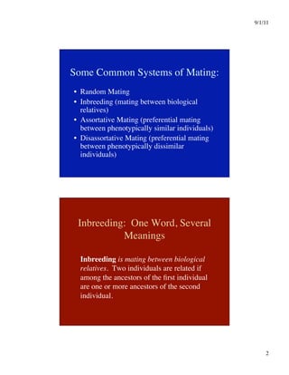
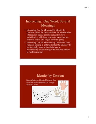
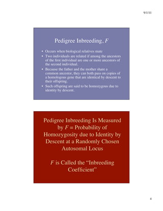
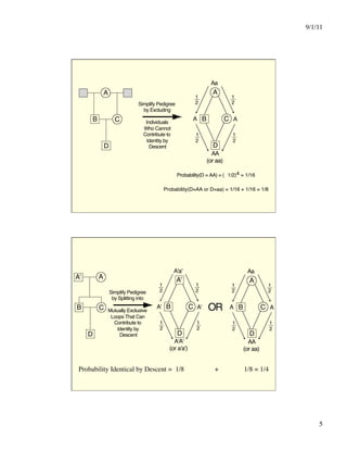
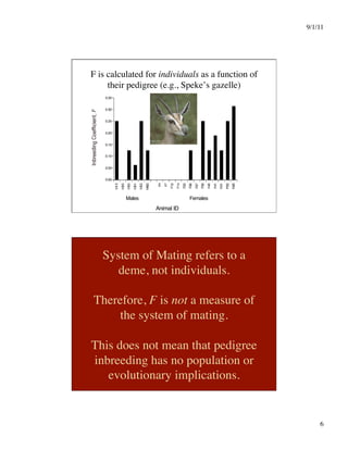
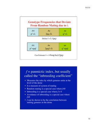
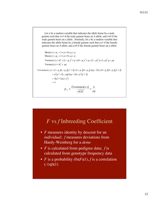
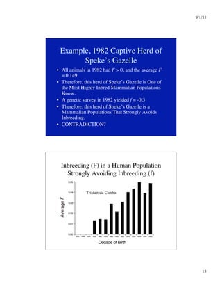
9/1/11

1

Systems of Mating:
the rules by which pairs of
gametes are chosen from the
local gene pool to be united in a
zygote with respect to a particular
locus or genetic system.
Systems of Mating:
A deme is not defined by geography but rather by
a shared system of mating. Depending upon the
geographical scale involved and the individuals’
dispersal and mating abilities, a deme may
correspond to the entire species or to a
subpopulation restricted to a small local region.
The Hardy-Weinberg model assumes one
particular system of mating – random mating –
but many other systems of mating exist.
9/1/11

2

Some Common Systems of Mating:
•  Random Mating
•  Inbreeding (mating between biological
relatives)
•  Assortative Mating (preferential mating
between phenotypically similar individuals)
•  Disassortative Mating (preferential mating
between phenotypically dissimilar
individuals)
Inbreeding: One Word, Several
Meanings

Inbreeding is mating between biological
relatives. Two individuals are related if
among the ancestors of the first individual
are one or more ancestors of the second
individual.
9/1/11

3

Inbreeding: One Word, Several
Meanings
•  Inbreeding Can Be Measured by Identity by
Descent, Either for Individuals or for a Population
(Because of shared common ancestors, two
individuals could share genes at a locus that are
identical copies of a single ancestral gene)
•  Inbreeding Can Be Measured by Deviations from
Random Mating in a Deme (either the tendency to
preferentially mate with relatives or to
preferentially avoid mating with relatives relative
to random mating)
Identity by Descent
Some alleles are identical because they
are replicated descendants of a single
ancestral allele
9/1/11

4

Pedigree Inbreeding, F
•  Occurs when biological relatives mate
•  Two individuals are related if among the ancestors
of the first individual are one or more ancestors of
the second individual.
•  Because the father and the mother share a
common ancestor, they can both pass on copies of
a homologous gene that are identical by descent to
their offspring.
•  Such offspring are said to be homozygous due to
identity by descent.
Pedigree Inbreeding Is Measured
by F = Probability of
Homozygosity due to Identity by
Descent at a Randomly Chosen
Autosomal Locus
F is Called the “Inbreeding
Coefficient”
9/1/11

5

A
B C
D
Simplify Pedigree
by Excluding
Individuals
Who Cannot
Contribute to
Identity by
Descent
A
B C
D
Aa
A A
AA
(or aa)
1
2
1
2
1
2
1
2
Probability(D = AA) = ( 1/2)4 = 1/16
Probability(D=AA or D=aa) = 1/16 + 1/16 = 1/8
A
B C
D
Simplify Pedigree
by Splitting into
Mutually Exclusive
Loops That Can
Contribute to
Identity by
Descent
A
B C
D
Aa
A A
AA
(or aa)
1
2
1
2
1
2
1
2
A'
B C
D
A'a'
A' A'
A'A'
(or a'a')
1
2
1
2
1
2
1
2
A'
OR
Probability Identical by Descent = 1/8 + 1/8 = 1/4
9/1/11

6

F is calculated for individuals as a function of
their pedigree (e.g., Speke’s gazelle)
Animal ID
Males Females
0.35
0.30
0.25
0.20
0.15
0.10
0.05
0.00
System of Mating refers to a
deme, not individuals.
Therefore, F is not a measure of
the system of mating.
This does not mean that pedigree
inbreeding has no population or
evolutionary implications.
9/1/11

7

F displays strong interactions with rare, recessive
alleles and epistatic gene complexes.

Consider first a model in which a recessive allele is lethal when
homozygous.

• B = the sum over all loci of the probability that a gamete drawn
from the gene pool bears a recessive lethal allele at a particular
locus.
• Alternatively, B = the average number of lethal alleles over all loci
borne by a gamete in the gene pool.
• BF = the rate of occurrence of both gametes bearing lethal alleles
that are identical by descent, thereby resulting in the death of the
inbred individual. 
Consider first a model in which a recessive allele is
lethal when homozygous.

• The number of times an inbred individual will be identical-by-
descent for a lethal allele will often follow a Poisson distribution.
• e‑BF = the probability that an individual has exactly 0 lethal genes
that are identical-by-descent and therefore homozygous.
• -A = the natural logarithm of the probability of not dying from any
cause other then being homozgyous for a lethal recessive allele that
is identical-by-descent, so e‑A = the probability of not dying from
something else.
• e‑BFe‑A = e-(A+BF) = probability of an individual with F being alive.
• ln(Probability of an individual with F being alive) = -A - BF
9/1/11

8

Consider first a model in which a recessive allele is
lethal when homozygous.

• ln(Probability of an individual with F being alive) = -A - BF
• Because BF0, the above equation describes inbreeding
depression, the reduction of a beneficial trait (such as viability or
birth weight) with increasing levels of pedigree inbreeding. 
• To detect and describe inbreeding depression, pool together all the
animals in a population with the same F to estimate the probability
of being alive, and then regress the ln(prob. of being alive) vs. F.
100
90
80
70
60
50
40
30
25
0 1/16
1/8
3/16
1/4
5/16
Inbreeding Coefficient ( F)
30 Day Survival
1 Year Survival
A = -ln(0.79)=0.23
A = -ln(0.66)
=0.42
Inbreeding Depression in Speke’s gazelle
9/1/11

9

F displays strong interactions with rare, recessive
alleles and epistatic gene complexes.

Example of epistasis: synthetic lethals.

• Knock-out (complete loss of function) mutations were induced for
virtually all of the 6200 genes in the yeast (Saccharomyces
cerevisiae) genome (Tong et al. 2001. Sci. 294:2364-2368).
• 80% of these knock-out mutations were not lethal when made
homozygous through identity by descent and classified
“nonessential”
• Extensive lethality emerged when yeast strains were bred that bore
homozygous pairs of mutants from this “nonessential” class.
• Therefore, B = the number of “lethal equivalents” rather than the
number of actual lethal alleles.
F displays strong interactions with rare, recessive
alleles and epistatic gene complexes.

• 2B = the number of lethal equivalents in heterozygous condition
that a living animal is expected to bear.
• For Speke’s gazelles, the average number of lethal equivalents for
one-year survivorship borne by the founding animals of this herd is
therefore 7.5 lethal equivalents per animal.
• Humans from the United States and Europe yield values of 2B
between 5-8.
• Therefore, even small amounts of pedigree inbreeding in a
population may increase the incidence of some types of genetic
disease by orders of magnitude in the pedigree-inbred subset of the
population (e.g., 0.05% of matings in the US are between cousins,
but 18-24% of albinos in the US come from cousin matings vs. an
overall incidence of 0.006%).
9/1/11

10

System of Mating Inbreeding, f
•  F is calculated for individuals from pedigree
data.
•  Demes are defined by a shared system of
mating, but this is a population level concept.
•  Therefore, we need another definition of
inbreeding at the level of a deme to describe
the population incidence of matings between
relatives.
Inbreeding as a Deviation from Random Mating
A
p
a
q
A
p
AA
p2 +λ
Aa
pq-λ
a
q
aA
qp-λ
aa
q2 +λ
A
p
a
q = 1-p
Maternal Gamete
Paternal
Gamete
Gene Pool
9/1/11

11

Genotype Frequencies that Deviate
From Random Mating due to λ
AA
p2 +λ
Aa
2pq-2λ
aa
q2 +λ
Define f = λ /(pq)
AA
p2 +pqf
Aa
2pq(1-f)
aa
q2 +pqf
Can Estimate f = 1-Freq(Aa)/(2pq)
f = panmictic index, but usually
called the “inbreeding coefficient”
•  Measures the rules by which gametes unite at the
level of the deme
•  Is a measure of system of mating
•  Random mating is a special case where f=0
•  Inbreeding is a special case where f  0
•  Avoidance of inbreeding is a special case where
f0
•  f can be shown to be the correlation between
uniting gametes in the deme
9/1/11

12

Let x be a random variable that indicates the allele borne by a male
gamete such that x=1 if the male gamete bears an A allele, and x=0 if the
male gamete bears an a allele. Similarly, let y be a random variable that
indicates the allele borne by a female gamete such that y=1 if the female
gamete bears an A allele, and y=0 if the female gamete bears an a allele.
Mean(x) = µx = 1× p + 0× q = p
Mean(y) = µy = 1× p + 0× q = p
Variance(x) = σx
2
= 1− µx
( )
2
× p + 0− µx
( )
2
× q = 1− p
( )
2
p + − p
( )
2
q = pq
Variance(y) = σy
2
= pq
Covariance(x,y) = 1− µx
( ) 1− µy
( ) p2
+ λ
( )+ 1− µx
( ) 0− µy
( ) 2pq− 2λ
( )+ 0− µx
( ) 0− µy
( ) q2
+ λ
( )
= q2
p2
+ λ
( )− pq 2pq− 2λ
( )+ p2
q2
+ λ
( )
= λ q2
+ 2pq+ p2
( )
= λ
ρx, y =
Covariance x,y
( )
σx
2
σy
2
=
λ
pq
F vs f Inbreeding Coefficient
•  F measures identity by descent for an
individual; f measures deviations from
Hardy-Weinberg for a deme
•  F is calculated from pedigree data; f is
calculated from genotype frequency data
•  F is a probability (0≤F≤1), f is a correlation
(-1≤f≤1)
9/1/11

13

Example, 1982 Captive Herd of
Speke’s Gazelle
•  All animals in 1982 had F  0, and the average F
= 0.149
•  Therefore, this herd of Speke’s Gazelle is One of
the Most Highly Inbred Mammalian Populations
Know.
•  A genetic survey in 1982 yielded f = -0.3
•  Therefore, this herd of Speke’s Gazelle is a
Mammalian Populations That Strongly Avoids
Inbreeding.
•  CONTRADICTION? 
Inbreeding (F) in a Human Population
Strongly Avoiding Inbreeding (f)
0.00
0.01
0.02
0.03
0.04
0.05
1820 1830 1840 1850 1860 1870 1880 1890 1900 1910 1920 1930 1940 1950
Decade of Birth
Tristan da Cunha
9/1/11

14

Impact of f
•  Can greatly affect genotype frequencies,
particularly that of homozygotes for rare
alleles: e.g., let q =.001, then q2 = 0.000001
Now let f = 0.01, then q2+pqf = 0.000011
•  f is NOT an evolutionary force by itself: 
p’ = (1)(p2+pqf) + (.5)[2pq(1-f)]
= p2+pq + pqf - pqf
= p(p+q) = p
A contrast between F, the pedigree inbreeding coefficient,
and f, the system-of-mating inbreeding coefficient
Property
 F
 f
Data Used
 Pedigree Data
 Genotype
Frequency Data
Type of Measure
 Probability
 Correlation
Coefficient
Range
 0 ≤ F ≤ 1
 -1 ≤ f ≤ 1
Level
 Individual
 Deme
Biological
Meaning
Probability of
Identity–by–De-
scent
System of
Mating or HW
Deviation
9/1/11

15

Assortative Mating
occurs when individuals with similar
phenotypes are more likely to mate
than expected under random pairing
in the population
Assortative Mating
Reynolds, R. Graham  Fitzpatrick, Benjamin M. Evolution 61 (9), 2253-2259.
9/1/11

16

100% Assortative Mating For A Codominant, Single Locus Phenotype
1
 1
1/4

 1/4

Meiosis 
Fertilization
Phenotype
Production
Zygotes
1
Phenotypes of
Adult Population
1
 1
1
AA
GAA
Aa
GAa
aa
Gaa
TAA
GAA
TAa
GAa
Taa
Gaa
AA X AA
GAA
Aa X Aa
GAa
aa X aa
Gaa
Mate Choice
Mated Adults
AA
GAA+GAa/4
Aa
GAa/2
aa
Gaa+GAa/4
1
 1
1/2
Zygotes
100% Assortative Mating For A Codominant, Single Locus Phenotype
1
 1
1/4

 1/4

Zygotes
1
Phenotypes of
Adult Population
1
 1
1
AA
GAA
Aa
GAa
aa
Gaa
TAA
GAA
TAa
GAa
Taa
Gaa
AA X AA
GAA
Aa X Aa
GAa
aa X aa
Gaa
Mate Choice
Mated Adults
AA
GAA+GAa/4
Aa
GAa/2
aa
Gaa+GAa/4
1
 1
1/2
Zygotes
p = (1)GAA+(1/2)GAa
p’ = (1)(GAA+ GAa/4)+(1/2)GAa/2
p’ = GAA+ GAa/2 = p
9/1/11

17

100% Assortative Mating For A Codominant, Single Locus Phenotype
1/4

 1/4

Zygotes
Gen. 0
AA
GAA
Aa
GAa
aa
Gaa
AA
GAA+GAa/4
Aa
GAa/2
aa
Gaa+GAa/4
1
 1
1/2
Zygotes
Gen. 1
Note, GAa(1)= 1/2GAa(1) = GAa(i)= (1/2)iGAa(0) 
As i – ∞, GAa(equilibrium) – 0
At equilibrium:
aa
Gaa+GAa/2 = q
AA
GAA+GAa/2 = p
Profound, Early Onset Deafness
•  Assortative Mating Rates Vary From 80% to 94%
in USA and Europe.
•  About half of the cases are due to accidents and
disease
•  The other half of the cases are due to
homozygosity for a recessive allele at any one of
35 loci.
•  Half of the genetic cases are due to homozygosity
for a recessive allele at the GJB2 locus that
encodes the gap-junction protein connexin-26,
with q ≈ 0.01 in European and USA populations.
9/1/11

18

GJB2 locus, Alleles A and a
•  Frequency of a is about 0.01 in U.S.A. 
Europe
•  Under random mating expect an aa
genotype frequency of (0.01)2 = 0.0001 who
will be deaf
•  Actual incidence of deafness due to aa is
0.0003 to 0.0005 (as if f=0.02 to 0.04)
•  3 to 5 times more children are deaf due to
this gene because of assortative mating.
GJB2 locus, Alleles A and a
•  Only a quarter of the people with profound
early onset deafness are aa.
•  Within matings of deaf people, therefore
expect (1/4)(1/4) = 1/16 to be aa X aa.
•  But 1/6 of the children of deaf couples are aa!
•  In many of these couples, one of the parents is
deaf due to homozygosity for a recessive allele
at another locus, yet this person is also Aa at
the GJB2 locus.
9/1/11

19

GJB2 locus, Alleles A and a
•  Consider a second locus with alleles B and b such
that bb is deaf and frequency of b is 0.0001.
•  Under random mating equilibrium, expected
frequency of ab gametes is (0.01)(0.0001) =
0.000001
•  But assortative mating implies that the rare bb
individuals will mate 1/4 of the time with aa
individuals, and the children of such matings can
produce ab gametes.
•  THEREFORE, ASSORTATIVE MATING
CREATES LINKAGE DISEQUILIBRIUM!
2-Locus, 2-Allele 100% Assortative Mating With Additive Phenotypes
9/1/11

20

Equilibrium Populations Possible Under
a 2-Locus, 2-Allele 100% Assortative
Mating With Additive Phenotypes
Initial Gene Pool
Genotypes pA = pB pA  pB pA  pB
AB/AB pA pA pB
Ab/Ab 0 0 pA - pB
aB/aB 0 pB - pA 0
ab/ab pb pb pa
Note, can start with D=0, but all equilibrium populations have |D’|=1

Properties of Assortative Mating
•  Increases the Frequency of Homozygotes Relative to
Hardy-Weinberg For Loci Contributing to the
Phenotype Or For Loci Correlated For Any Reason to
the Phenotype
•  Does Not Change Allele Frequencies --Therefore Is Not
An Evolutionary Forces at the Single Locus Level
•  Assortative Mating Creates Disequilibrium Among Loci
that Contribute to the Phenotype and Is A Powerful
Evolutionary Force at the Multi-Locus Level
•  Multiple Equilibria Exist at the Multi-Locus Level And
The Course of Evolution Is Constrained By the Initial
Gene Pool: historical factors are a determinant of the
course of evolution
9/1/11

21

Assortative Mating  Inbreeding
•  Both Increase Frequency of Homozygotes Relative to
Hardy-Weinberg (result in f  0)
•  Increased Homozygosity Under Assortative Mating
Occurs Only For Loci Contributing to the Phenotype Or
For Loci Correlated For Any Reason to the Phenotype;
Inbreeding Increases Homozygosity for All Loci
•  Neither Changes Allele Frequencies --Therefore They
Are Not Evolutionary Forces at the Single Locus Level
•  Assortative Mating Creates Disequilibrium Among Loci
that Contribute to the Phenotype; Inbreeding Slows
Down the Decay of Disequilibrium, but Does Not
Create Any Disequilibrium.
ASSORTATIVE MATING, LINKAGE
DISEQUILIBRIUM AND ADMIXTURE
•  Assortative mating directly affects the genotype and
gamete frequencies of the loci that contribute to the
phenotype for which assortative mating is occurring and
of any loci in linkage disequilibrium with them.
•  Admixture occurs when two or more genetically
distinct subpopulations are mixed together and begin
interbreeding.
•  Admixture induces disequilibrium, so assortative mating
for any phenotype associated with the parental
subpopulations can potentially affect the genotype
frequencies at many loci not directly affect the assorting
phenotype.
9/1/11

22

ASSORTATIVE MATING, LINKAGE
DISEQUILIBRIUM AND ADMIXTURE
Subpopulation 1
0.03
 0.07
 0.27
 0.63
 0.63
 0.27
 0.07
0.03
Subpopulation 2
D = (0.03)(0.63)-(0.07)(0.27) = 0
 D = (0.63)(0.03)-(0.27)(0.07) = 0
Combined Population (50:50 Mix)
0.33
 0.17
 0.17
 0.33
D = (0.33)(0.33)-(0.17)(0.17) = 0.08
AB

 Ab
 aB
 ab
 AB

 Ab
 aB
 ab
AB

 Ab
 aB
 ab
ASSORTATIVE MATING, LINKAGE
DISEQUILIBRIUM AND ADMIXTURE
•  Assortative mating for any trait that differentiates the
original subpopulations (even non genetic) reduces
heterozygosity at all loci with allele frequency
differences between the original subpopulations.
•  The rate of dissipation of D in the admixed population is
therefore  (1-r). 
•  The admixed populations do not fuse immediately, but
rather remain stratified, sometimes indefinitely if the
assortative mating is strong enough.
9/1/11

23

Disassortative Mating
occurs when individuals with
dissimilar phenotypes are more likely
to mate than expected under random
pairing in the population
Disassortative Mating
Cowslip
9/1/11

24

Disassortative Mating
Cowslip
Disassortative Mating
Cowslip
9/1/11

25

A model of 100% Disassortative mating
Disassortative Mating Starting at HW Equilibrium
generation AA Aa aa p f
0 0.5625 0.3750 0.0625 0.7500 0.0000
1 0.3913 0.5652 0.0435 0.6739 -0.2860
2 0.4209 0.5324 0.0468 0.6871 -0.2380
3 0.4170 0.5366 0.0463 0.6853 -0.2442
4 0.4176 0.5361 0.0464 0.6856 -0.2434
5 0.4175 0.5361 0.0464 0.6855 -0.2435
6 0.4175 0.5361 0.0464 0.6856 -0.2435
7 0.4175 0.5361 0.0464 0.6856 -0.2435
8 0.4175 0.5361 0.0464 0.6856 -0.2435
9 0.4175 0.5361 0.0464 0.6856 -0.2435
10 0.4175 0.5361 0.0464 0.6856 -0.2435
11 0.4175 0.5361 0.0464 0.6856 -0.2435
12 0.4175 0.5361 0.0464 0.6856 -0.2435
13 0.4175 0.5361 0.0464 0.6856 -0.2435
9/1/11

26

Disassortative Mating Starting at HW Equilibrium
generation AA Aa aa p f
0 0.0625 0.3750 0.5625 0.2500 0.0000
1 0.0435 0.5652 0.3913 0.3261 -0.2860
2 0.0468 0.5324 0.4209 0.3129 -0.2380
3 0.0463 0.5366 0.4170 0.3147 -0.2442
4 0.0464 0.5361 0.4176 0.3144 -0.2434
5 0.0464 0.5361 0.4175 0.3145 -0.2435
6 0.0464 0.5361 0.4175 0.3144 -0.2435
7 0.0464 0.5361 0.4175 0.3144 -0.2435
8 0.0464 0.5361 0.4175 0.3144 -0.2435
9 0.0464 0.5361 0.4175 0.3144 -0.2435
10 0.0464 0.5361 0.4175 0.3144 -0.2435
11 0.0464 0.5361 0.4175 0.3144 -0.2435
12 0.0464 0.5361 0.4175 0.3144 -0.2435
13 0.0464 0.5361 0.4175 0.3144 -0.2435
Note, the Equilibrium depends upon the starting conditions; multiple
polymorphic equilibria are common with disassortative mating

Disassortative Mating as an
Evolutionary Force
•  Is a powerful evolutionary force at the single locus
level, generally resulting in stable equilibrium
populations with intermediate allele frequencies and
f0
•  It is less powerful as an evolutionary force at the multi-
locus level because it produces a heterozygote excess,
which allows linkage disequilibrium to break down
more rapidly
•  Mimics the heterozygote excess of avoidance of
inbreeding, but unlike avoidance of inbreeding, it
affects only those loci correlated with the relevant
phenotype, and it causes allele frequency change.
9/1/11

27

Disassortative Mating and Admixture
•  Disassortative mating amplifies gene flow between the
parental subpopulations.
•  Therefore, disassortative mating rapidly destroys
genetic differences between historical
subpopulations
•  Disassortative mating increases heterozygosity above
random mating expectations for all loci with initial
allele frequency differences between the parental
subpopulations, and hence D dissipates at a rate  (1-r).
•  Therefore, disassortative mating rapidly destroys
the linkage disequilibrium created by admixture.
Disassortative Mating and Admixture
9/1/11

28

Disassortative Mating and Admixture
Diagnostic
Allele
Yanomama
 Borabuk
Yanomama
Makiritare
Dia
 0.00
 0.06
 0.04
Apa
 0.00
 0.08
 0.05
Systems of Matings
Systems of mating can be potent
evolutionary forces, both by
themselves and in interactions with
other evolutionary factors. In
subsequent lectures we will examine
additional interactions between
system of mating and other
evolutionary forces.

Hardy Weinberg

  • 1.
    9/1/11 1 Systems of Mating: therules by which pairs of gametes are chosen from the local gene pool to be united in a zygote with respect to a particular locus or genetic system. Systems of Mating: A deme is not defined by geography but rather by a shared system of mating. Depending upon the geographical scale involved and the individuals’ dispersal and mating abilities, a deme may correspond to the entire species or to a subpopulation restricted to a small local region. The Hardy-Weinberg model assumes one particular system of mating – random mating – but many other systems of mating exist.
  • 2.
    9/1/11 2 Some Common Systemsof Mating: •  Random Mating •  Inbreeding (mating between biological relatives) •  Assortative Mating (preferential mating between phenotypically similar individuals) •  Disassortative Mating (preferential mating between phenotypically dissimilar individuals) Inbreeding: One Word, Several Meanings Inbreeding is mating between biological relatives. Two individuals are related if among the ancestors of the first individual are one or more ancestors of the second individual.
  • 3.
    9/1/11 3 Inbreeding: One Word,Several Meanings •  Inbreeding Can Be Measured by Identity by Descent, Either for Individuals or for a Population (Because of shared common ancestors, two individuals could share genes at a locus that are identical copies of a single ancestral gene) •  Inbreeding Can Be Measured by Deviations from Random Mating in a Deme (either the tendency to preferentially mate with relatives or to preferentially avoid mating with relatives relative to random mating) Identity by Descent Some alleles are identical because they are replicated descendants of a single ancestral allele
  • 4.
    9/1/11 4 Pedigree Inbreeding, F • Occurs when biological relatives mate •  Two individuals are related if among the ancestors of the first individual are one or more ancestors of the second individual. •  Because the father and the mother share a common ancestor, they can both pass on copies of a homologous gene that are identical by descent to their offspring. •  Such offspring are said to be homozygous due to identity by descent. Pedigree Inbreeding Is Measured by F = Probability of Homozygosity due to Identity by Descent at a Randomly Chosen Autosomal Locus F is Called the “Inbreeding Coefficient”
  • 5.
    9/1/11 5 A B C D Simplify Pedigree byExcluding Individuals Who Cannot Contribute to Identity by Descent A B C D Aa A A AA (or aa) 1 2 1 2 1 2 1 2 Probability(D = AA) = ( 1/2)4 = 1/16 Probability(D=AA or D=aa) = 1/16 + 1/16 = 1/8 A B C D Simplify Pedigree by Splitting into Mutually Exclusive Loops That Can Contribute to Identity by Descent A B C D Aa A A AA (or aa) 1 2 1 2 1 2 1 2 A' B C D A'a' A' A' A'A' (or a'a') 1 2 1 2 1 2 1 2 A' OR Probability Identical by Descent = 1/8 + 1/8 = 1/4
  • 6.
    9/1/11 6 F is calculatedfor individuals as a function of their pedigree (e.g., Speke’s gazelle) Animal ID Males Females 0.35 0.30 0.25 0.20 0.15 0.10 0.05 0.00 System of Mating refers to a deme, not individuals. Therefore, F is not a measure of the system of mating. This does not mean that pedigree inbreeding has no population or evolutionary implications.
  • 7.
    9/1/11 7 F displays stronginteractions with rare, recessive alleles and epistatic gene complexes. Consider first a model in which a recessive allele is lethal when homozygous. • B = the sum over all loci of the probability that a gamete drawn from the gene pool bears a recessive lethal allele at a particular locus. • Alternatively, B = the average number of lethal alleles over all loci borne by a gamete in the gene pool. • BF = the rate of occurrence of both gametes bearing lethal alleles that are identical by descent, thereby resulting in the death of the inbred individual. Consider first a model in which a recessive allele is lethal when homozygous. • The number of times an inbred individual will be identical-by- descent for a lethal allele will often follow a Poisson distribution. • e‑BF = the probability that an individual has exactly 0 lethal genes that are identical-by-descent and therefore homozygous. • -A = the natural logarithm of the probability of not dying from any cause other then being homozgyous for a lethal recessive allele that is identical-by-descent, so e‑A = the probability of not dying from something else. • e‑BFe‑A = e-(A+BF) = probability of an individual with F being alive. • ln(Probability of an individual with F being alive) = -A - BF
  • 8.
    9/1/11 8 Consider first amodel in which a recessive allele is lethal when homozygous. • ln(Probability of an individual with F being alive) = -A - BF • Because BF0, the above equation describes inbreeding depression, the reduction of a beneficial trait (such as viability or birth weight) with increasing levels of pedigree inbreeding. • To detect and describe inbreeding depression, pool together all the animals in a population with the same F to estimate the probability of being alive, and then regress the ln(prob. of being alive) vs. F. 100 90 80 70 60 50 40 30 25 0 1/16 1/8 3/16 1/4 5/16 Inbreeding Coefficient ( F) 30 Day Survival 1 Year Survival A = -ln(0.79)=0.23 A = -ln(0.66) =0.42 Inbreeding Depression in Speke’s gazelle
  • 9.
    9/1/11 9 F displays stronginteractions with rare, recessive alleles and epistatic gene complexes. Example of epistasis: synthetic lethals. • Knock-out (complete loss of function) mutations were induced for virtually all of the 6200 genes in the yeast (Saccharomyces cerevisiae) genome (Tong et al. 2001. Sci. 294:2364-2368). • 80% of these knock-out mutations were not lethal when made homozygous through identity by descent and classified “nonessential” • Extensive lethality emerged when yeast strains were bred that bore homozygous pairs of mutants from this “nonessential” class. • Therefore, B = the number of “lethal equivalents” rather than the number of actual lethal alleles. F displays strong interactions with rare, recessive alleles and epistatic gene complexes. • 2B = the number of lethal equivalents in heterozygous condition that a living animal is expected to bear. • For Speke’s gazelles, the average number of lethal equivalents for one-year survivorship borne by the founding animals of this herd is therefore 7.5 lethal equivalents per animal. • Humans from the United States and Europe yield values of 2B between 5-8. • Therefore, even small amounts of pedigree inbreeding in a population may increase the incidence of some types of genetic disease by orders of magnitude in the pedigree-inbred subset of the population (e.g., 0.05% of matings in the US are between cousins, but 18-24% of albinos in the US come from cousin matings vs. an overall incidence of 0.006%).
  • 10.
    9/1/11 10 System of MatingInbreeding, f •  F is calculated for individuals from pedigree data. •  Demes are defined by a shared system of mating, but this is a population level concept. •  Therefore, we need another definition of inbreeding at the level of a deme to describe the population incidence of matings between relatives. Inbreeding as a Deviation from Random Mating A p a q A p AA p2 +λ Aa pq-λ a q aA qp-λ aa q2 +λ A p a q = 1-p Maternal Gamete Paternal Gamete Gene Pool
  • 11.
    9/1/11 11 Genotype Frequencies thatDeviate From Random Mating due to λ AA p2 +λ Aa 2pq-2λ aa q2 +λ Define f = λ /(pq) AA p2 +pqf Aa 2pq(1-f) aa q2 +pqf Can Estimate f = 1-Freq(Aa)/(2pq) f = panmictic index, but usually called the “inbreeding coefficient” •  Measures the rules by which gametes unite at the level of the deme •  Is a measure of system of mating •  Random mating is a special case where f=0 •  Inbreeding is a special case where f 0 •  Avoidance of inbreeding is a special case where f0 •  f can be shown to be the correlation between uniting gametes in the deme
  • 12.
    9/1/11 12 Let x bea random variable that indicates the allele borne by a male gamete such that x=1 if the male gamete bears an A allele, and x=0 if the male gamete bears an a allele. Similarly, let y be a random variable that indicates the allele borne by a female gamete such that y=1 if the female gamete bears an A allele, and y=0 if the female gamete bears an a allele. Mean(x) = µx = 1× p + 0× q = p Mean(y) = µy = 1× p + 0× q = p Variance(x) = σx 2 = 1− µx ( ) 2 × p + 0− µx ( ) 2 × q = 1− p ( ) 2 p + − p ( ) 2 q = pq Variance(y) = σy 2 = pq Covariance(x,y) = 1− µx ( ) 1− µy ( ) p2 + λ ( )+ 1− µx ( ) 0− µy ( ) 2pq− 2λ ( )+ 0− µx ( ) 0− µy ( ) q2 + λ ( ) = q2 p2 + λ ( )− pq 2pq− 2λ ( )+ p2 q2 + λ ( ) = λ q2 + 2pq+ p2 ( ) = λ ρx, y = Covariance x,y ( ) σx 2 σy 2 = λ pq F vs f Inbreeding Coefficient •  F measures identity by descent for an individual; f measures deviations from Hardy-Weinberg for a deme •  F is calculated from pedigree data; f is calculated from genotype frequency data •  F is a probability (0≤F≤1), f is a correlation (-1≤f≤1)
  • 13.
    9/1/11 13 Example, 1982 CaptiveHerd of Speke’s Gazelle •  All animals in 1982 had F 0, and the average F = 0.149 •  Therefore, this herd of Speke’s Gazelle is One of the Most Highly Inbred Mammalian Populations Know. •  A genetic survey in 1982 yielded f = -0.3 •  Therefore, this herd of Speke’s Gazelle is a Mammalian Populations That Strongly Avoids Inbreeding. •  CONTRADICTION? Inbreeding (F) in a Human Population Strongly Avoiding Inbreeding (f) 0.00 0.01 0.02 0.03 0.04 0.05 1820 1830 1840 1850 1860 1870 1880 1890 1900 1910 1920 1930 1940 1950 Decade of Birth Tristan da Cunha
  • 14.
    9/1/11 14 Impact of f • Can greatly affect genotype frequencies, particularly that of homozygotes for rare alleles: e.g., let q =.001, then q2 = 0.000001 Now let f = 0.01, then q2+pqf = 0.000011 •  f is NOT an evolutionary force by itself: p’ = (1)(p2+pqf) + (.5)[2pq(1-f)] = p2+pq + pqf - pqf = p(p+q) = p A contrast between F, the pedigree inbreeding coefficient, and f, the system-of-mating inbreeding coefficient Property F f Data Used Pedigree Data Genotype Frequency Data Type of Measure Probability Correlation Coefficient Range 0 ≤ F ≤ 1 -1 ≤ f ≤ 1 Level Individual Deme Biological Meaning Probability of Identity–by–De- scent System of Mating or HW Deviation
  • 15.
    9/1/11 15 Assortative Mating occurs whenindividuals with similar phenotypes are more likely to mate than expected under random pairing in the population Assortative Mating Reynolds, R. Graham Fitzpatrick, Benjamin M. Evolution 61 (9), 2253-2259.
  • 16.
    9/1/11 16 100% Assortative MatingFor A Codominant, Single Locus Phenotype 1 1 1/4 1/4 Meiosis Fertilization Phenotype Production Zygotes 1 Phenotypes of Adult Population 1 1 1 AA GAA Aa GAa aa Gaa TAA GAA TAa GAa Taa Gaa AA X AA GAA Aa X Aa GAa aa X aa Gaa Mate Choice Mated Adults AA GAA+GAa/4 Aa GAa/2 aa Gaa+GAa/4 1 1 1/2 Zygotes 100% Assortative Mating For A Codominant, Single Locus Phenotype 1 1 1/4 1/4 Zygotes 1 Phenotypes of Adult Population 1 1 1 AA GAA Aa GAa aa Gaa TAA GAA TAa GAa Taa Gaa AA X AA GAA Aa X Aa GAa aa X aa Gaa Mate Choice Mated Adults AA GAA+GAa/4 Aa GAa/2 aa Gaa+GAa/4 1 1 1/2 Zygotes p = (1)GAA+(1/2)GAa p’ = (1)(GAA+ GAa/4)+(1/2)GAa/2 p’ = GAA+ GAa/2 = p
  • 17.
    9/1/11 17 100% Assortative MatingFor A Codominant, Single Locus Phenotype 1/4 1/4 Zygotes Gen. 0 AA GAA Aa GAa aa Gaa AA GAA+GAa/4 Aa GAa/2 aa Gaa+GAa/4 1 1 1/2 Zygotes Gen. 1 Note, GAa(1)= 1/2GAa(1) = GAa(i)= (1/2)iGAa(0) As i – ∞, GAa(equilibrium) – 0 At equilibrium: aa Gaa+GAa/2 = q AA GAA+GAa/2 = p Profound, Early Onset Deafness •  Assortative Mating Rates Vary From 80% to 94% in USA and Europe. •  About half of the cases are due to accidents and disease •  The other half of the cases are due to homozygosity for a recessive allele at any one of 35 loci. •  Half of the genetic cases are due to homozygosity for a recessive allele at the GJB2 locus that encodes the gap-junction protein connexin-26, with q ≈ 0.01 in European and USA populations.
  • 18.
    9/1/11 18 GJB2 locus, AllelesA and a •  Frequency of a is about 0.01 in U.S.A. Europe •  Under random mating expect an aa genotype frequency of (0.01)2 = 0.0001 who will be deaf •  Actual incidence of deafness due to aa is 0.0003 to 0.0005 (as if f=0.02 to 0.04) •  3 to 5 times more children are deaf due to this gene because of assortative mating. GJB2 locus, Alleles A and a •  Only a quarter of the people with profound early onset deafness are aa. •  Within matings of deaf people, therefore expect (1/4)(1/4) = 1/16 to be aa X aa. •  But 1/6 of the children of deaf couples are aa! •  In many of these couples, one of the parents is deaf due to homozygosity for a recessive allele at another locus, yet this person is also Aa at the GJB2 locus.
  • 19.
    9/1/11 19 GJB2 locus, AllelesA and a •  Consider a second locus with alleles B and b such that bb is deaf and frequency of b is 0.0001. •  Under random mating equilibrium, expected frequency of ab gametes is (0.01)(0.0001) = 0.000001 •  But assortative mating implies that the rare bb individuals will mate 1/4 of the time with aa individuals, and the children of such matings can produce ab gametes. •  THEREFORE, ASSORTATIVE MATING CREATES LINKAGE DISEQUILIBRIUM! 2-Locus, 2-Allele 100% Assortative Mating With Additive Phenotypes
  • 20.
    9/1/11 20 Equilibrium Populations PossibleUnder a 2-Locus, 2-Allele 100% Assortative Mating With Additive Phenotypes Initial Gene Pool Genotypes pA = pB pA pB pA pB AB/AB pA pA pB Ab/Ab 0 0 pA - pB aB/aB 0 pB - pA 0 ab/ab pb pb pa Note, can start with D=0, but all equilibrium populations have |D’|=1 Properties of Assortative Mating •  Increases the Frequency of Homozygotes Relative to Hardy-Weinberg For Loci Contributing to the Phenotype Or For Loci Correlated For Any Reason to the Phenotype •  Does Not Change Allele Frequencies --Therefore Is Not An Evolutionary Forces at the Single Locus Level •  Assortative Mating Creates Disequilibrium Among Loci that Contribute to the Phenotype and Is A Powerful Evolutionary Force at the Multi-Locus Level •  Multiple Equilibria Exist at the Multi-Locus Level And The Course of Evolution Is Constrained By the Initial Gene Pool: historical factors are a determinant of the course of evolution
  • 21.
    9/1/11 21 Assortative Mating Inbreeding •  Both Increase Frequency of Homozygotes Relative to Hardy-Weinberg (result in f 0) •  Increased Homozygosity Under Assortative Mating Occurs Only For Loci Contributing to the Phenotype Or For Loci Correlated For Any Reason to the Phenotype; Inbreeding Increases Homozygosity for All Loci •  Neither Changes Allele Frequencies --Therefore They Are Not Evolutionary Forces at the Single Locus Level •  Assortative Mating Creates Disequilibrium Among Loci that Contribute to the Phenotype; Inbreeding Slows Down the Decay of Disequilibrium, but Does Not Create Any Disequilibrium. ASSORTATIVE MATING, LINKAGE DISEQUILIBRIUM AND ADMIXTURE •  Assortative mating directly affects the genotype and gamete frequencies of the loci that contribute to the phenotype for which assortative mating is occurring and of any loci in linkage disequilibrium with them. •  Admixture occurs when two or more genetically distinct subpopulations are mixed together and begin interbreeding. •  Admixture induces disequilibrium, so assortative mating for any phenotype associated with the parental subpopulations can potentially affect the genotype frequencies at many loci not directly affect the assorting phenotype.
  • 22.
    9/1/11 22 ASSORTATIVE MATING, LINKAGE DISEQUILIBRIUMAND ADMIXTURE Subpopulation 1 0.03 0.07 0.27 0.63 0.63 0.27 0.07 0.03 Subpopulation 2 D = (0.03)(0.63)-(0.07)(0.27) = 0 D = (0.63)(0.03)-(0.27)(0.07) = 0 Combined Population (50:50 Mix) 0.33 0.17 0.17 0.33 D = (0.33)(0.33)-(0.17)(0.17) = 0.08 AB Ab aB ab AB Ab aB ab AB Ab aB ab ASSORTATIVE MATING, LINKAGE DISEQUILIBRIUM AND ADMIXTURE •  Assortative mating for any trait that differentiates the original subpopulations (even non genetic) reduces heterozygosity at all loci with allele frequency differences between the original subpopulations. •  The rate of dissipation of D in the admixed population is therefore (1-r). •  The admixed populations do not fuse immediately, but rather remain stratified, sometimes indefinitely if the assortative mating is strong enough.
  • 23.
    9/1/11 23 Disassortative Mating occurs whenindividuals with dissimilar phenotypes are more likely to mate than expected under random pairing in the population Disassortative Mating Cowslip
  • 24.
  • 25.
    9/1/11 25 A model of100% Disassortative mating Disassortative Mating Starting at HW Equilibrium generation AA Aa aa p f 0 0.5625 0.3750 0.0625 0.7500 0.0000 1 0.3913 0.5652 0.0435 0.6739 -0.2860 2 0.4209 0.5324 0.0468 0.6871 -0.2380 3 0.4170 0.5366 0.0463 0.6853 -0.2442 4 0.4176 0.5361 0.0464 0.6856 -0.2434 5 0.4175 0.5361 0.0464 0.6855 -0.2435 6 0.4175 0.5361 0.0464 0.6856 -0.2435 7 0.4175 0.5361 0.0464 0.6856 -0.2435 8 0.4175 0.5361 0.0464 0.6856 -0.2435 9 0.4175 0.5361 0.0464 0.6856 -0.2435 10 0.4175 0.5361 0.0464 0.6856 -0.2435 11 0.4175 0.5361 0.0464 0.6856 -0.2435 12 0.4175 0.5361 0.0464 0.6856 -0.2435 13 0.4175 0.5361 0.0464 0.6856 -0.2435
  • 26.
    9/1/11 26 Disassortative Mating Startingat HW Equilibrium generation AA Aa aa p f 0 0.0625 0.3750 0.5625 0.2500 0.0000 1 0.0435 0.5652 0.3913 0.3261 -0.2860 2 0.0468 0.5324 0.4209 0.3129 -0.2380 3 0.0463 0.5366 0.4170 0.3147 -0.2442 4 0.0464 0.5361 0.4176 0.3144 -0.2434 5 0.0464 0.5361 0.4175 0.3145 -0.2435 6 0.0464 0.5361 0.4175 0.3144 -0.2435 7 0.0464 0.5361 0.4175 0.3144 -0.2435 8 0.0464 0.5361 0.4175 0.3144 -0.2435 9 0.0464 0.5361 0.4175 0.3144 -0.2435 10 0.0464 0.5361 0.4175 0.3144 -0.2435 11 0.0464 0.5361 0.4175 0.3144 -0.2435 12 0.0464 0.5361 0.4175 0.3144 -0.2435 13 0.0464 0.5361 0.4175 0.3144 -0.2435 Note, the Equilibrium depends upon the starting conditions; multiple polymorphic equilibria are common with disassortative mating Disassortative Mating as an Evolutionary Force •  Is a powerful evolutionary force at the single locus level, generally resulting in stable equilibrium populations with intermediate allele frequencies and f0 •  It is less powerful as an evolutionary force at the multi- locus level because it produces a heterozygote excess, which allows linkage disequilibrium to break down more rapidly •  Mimics the heterozygote excess of avoidance of inbreeding, but unlike avoidance of inbreeding, it affects only those loci correlated with the relevant phenotype, and it causes allele frequency change.
  • 27.
    9/1/11 27 Disassortative Mating andAdmixture •  Disassortative mating amplifies gene flow between the parental subpopulations. •  Therefore, disassortative mating rapidly destroys genetic differences between historical subpopulations •  Disassortative mating increases heterozygosity above random mating expectations for all loci with initial allele frequency differences between the parental subpopulations, and hence D dissipates at a rate (1-r). •  Therefore, disassortative mating rapidly destroys the linkage disequilibrium created by admixture. Disassortative Mating and Admixture
  • 28.
    9/1/11 28 Disassortative Mating andAdmixture Diagnostic Allele Yanomama Borabuk Yanomama Makiritare Dia 0.00 0.06 0.04 Apa 0.00 0.08 0.05 Systems of Matings Systems of mating can be potent evolutionary forces, both by themselves and in interactions with other evolutionary factors. In subsequent lectures we will examine additional interactions between system of mating and other evolutionary forces.