This master's thesis investigates methods for computing multiple sense embeddings per polysemous word. The author extends the word2vec model to build a sense assignment model that simultaneously selects word senses in sentences and adapts the sense embedding vectors in an unsupervised learning approach. The model is implemented in Spark to enable training on large corpora. Sense vectors are trained on a Wikipedia corpus of nearly 1 billion tokens and evaluated on word similarity tasks using the SCWS and WordSim-353 datasets. Hyperparameter tuning is performed to analyze the effect of vector size, learning rate, and other parameters on model performance and training time. Nearest neighbors and example sentences are also examined to analyze the quality of the computed sense embeddings.


![Abstract
Recently, machine learning, and especially deep learning is very popular. Its main aim for
natural language processing to extract the meaning of words and sentences automatically.
The representation of words by a word vector is a very important tool for many natural
language processing tasks when using machine learning algorithms. There are many meth-
ods, e.g. [Mikolov et al., 2013]), to generate word vectors in such a way that semantically
similar words have similar word vectors of low distance. We call this process word embed-
ding, and these word vector a distributed representation. However, polysemous words can
have dierent meanings in dierent contexts. Accordingly, polysemous words should have
several vector representations for each sense. Some models have been recently proposed,
e.g. [Huang et al., 2012], to generate sense embeddings to represent word senses.
In our thesis we investigate and improve current methods to compute multiple sense em-
beddings per word. Specically we extend the basic word embedding model word2vec of
Mikolov et al. [2013] to build a sense assignment model. We use a score function to select
the best sense for each word in an unsupervised learning approach. Our model at the same
time selects senses for each word in sentences and adapts the sense embedding vectors. To
be able to train with large corpora we implement this model in Spark, a parallel execution
framework. We train sense vectors with a Wikipedia corpus of nearly 1 billion tokens. We
evaluate sense vectors by visualizing the semantic similarity of words and doing word simi-
larity tasks using the SCWS (Contextual Word Similarities) dataset and the WordSim-353
dataset from [Finkelstein et al., 2001].](https://image.slidesharecdn.com/eafda45f-0c51-4ed1-b9f3-f7670fd415ea-160726141620/75/HaiqingWang-MasterThesis-7-2048.jpg)


![List of Figures
1.1 Neigboring words dening the specic sense of bank. . . . . . . . . . . . 2
2.1 Graph of the tanh function . . . . . . . . . . . . . . . . . . . . . . . . . . . 6
2.2 An example of neural network with three layers . . . . . . . . . . . . . . . 7
2.3 The neural network structure from [Bengio et al., 2003] . . . . . . . . . . . 9
2.4 word2vec . . . . . . . . . . . . . . . . . . . . . . . . . . . . . . . . . . . . . 12
3.1 The network structure from [Huang et al., 2012] . . . . . . . . . . . . . . . 16
3.2 Architecture of MSSG model with window size Rt = 2 and S = 3 . . . . . 19
5.1 Shows the accumulated frequency of word count in range [1,51] . . . . . . . 30
5.2 Shows the accumulated frequency of word count in range [51,637] . . . . . 30
5.3 Shows the accumulated frequency of word count in range [637,31140] . . . 31
5.4 Shows the accumulated frequency of word count in range [31140,919787] . . 31
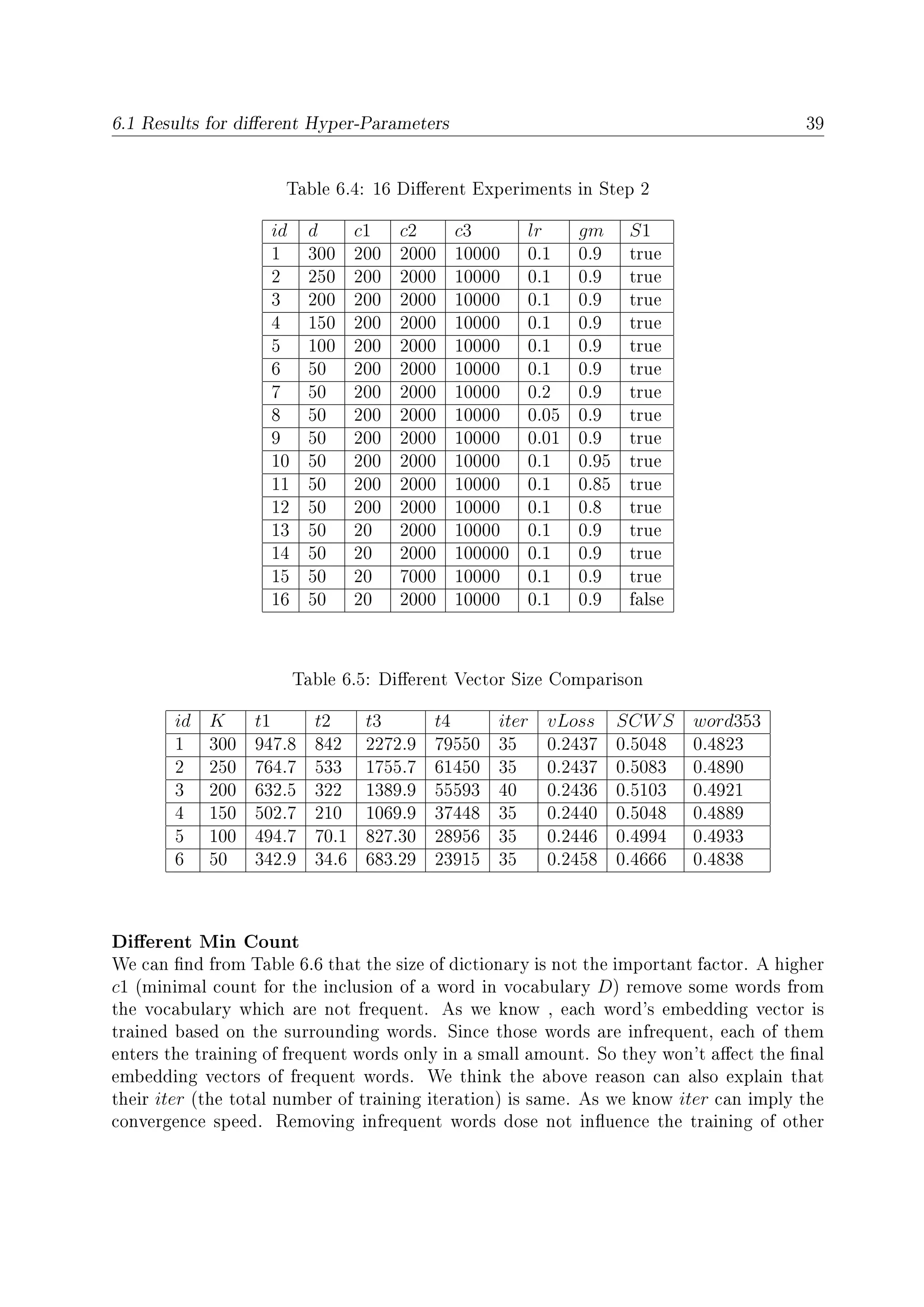
6.1 Shows the eect of varying embedding dimensionality of our model on the
Time . . . . . . . . . . . . . . . . . . . . . . . . . . . . . . . . . . . . . . . 40
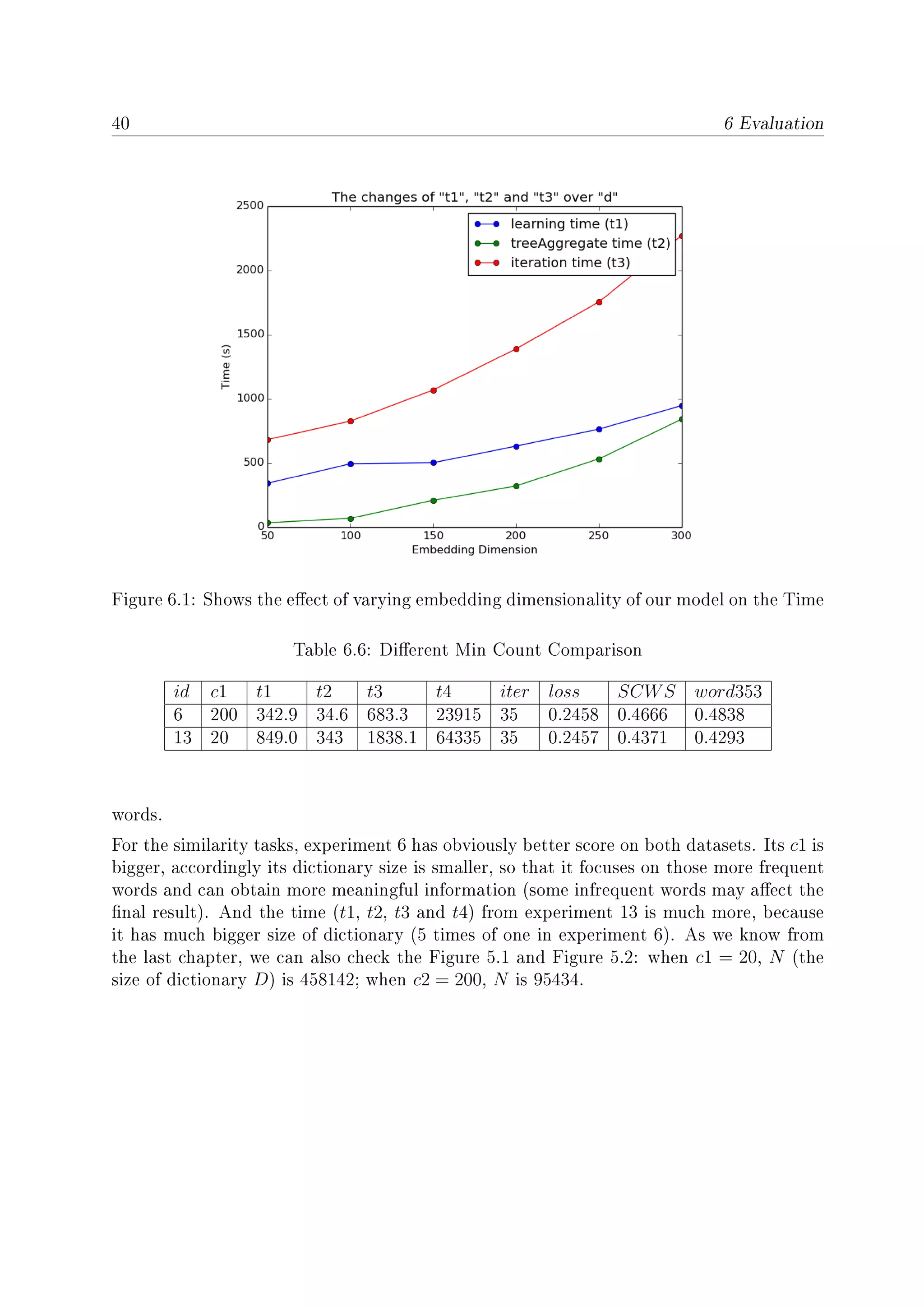
6.2 Shows the eect of varying embedding dimensionality of our model on the
loss of validation set . . . . . . . . . . . . . . . . . . . . . . . . . . . . . . 41
6.3 Shows the eect of varying embedding dimensionality of our model on the
SCWS task . . . . . . . . . . . . . . . . . . . . . . . . . . . . . . . . . . . 41
6.4 Shows the eect of varying embedding dimensionality of our model on the
WordSim-353 task . . . . . . . . . . . . . . . . . . . . . . . . . . . . . . . 42
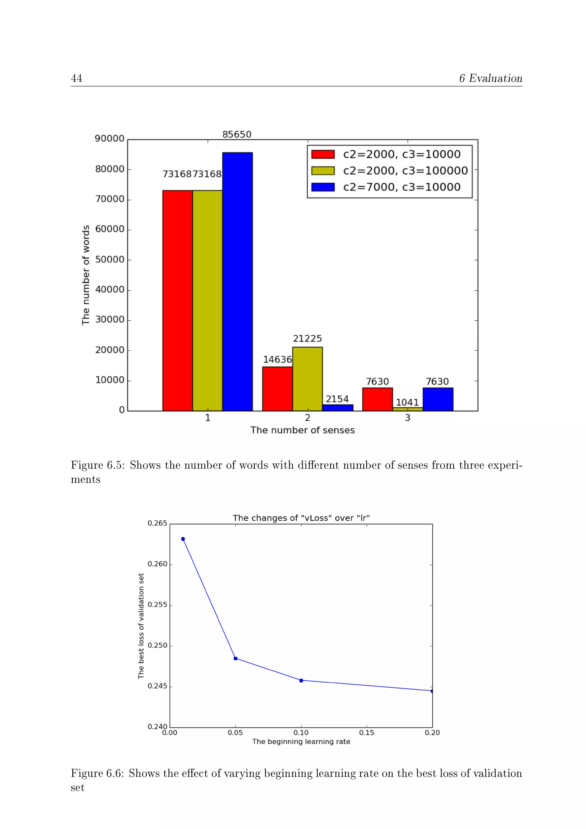
6.5 Shows the number of words with dierent number of senses from three ex-
periments . . . . . . . . . . . . . . . . . . . . . . . . . . . . . . . . . . . . 44
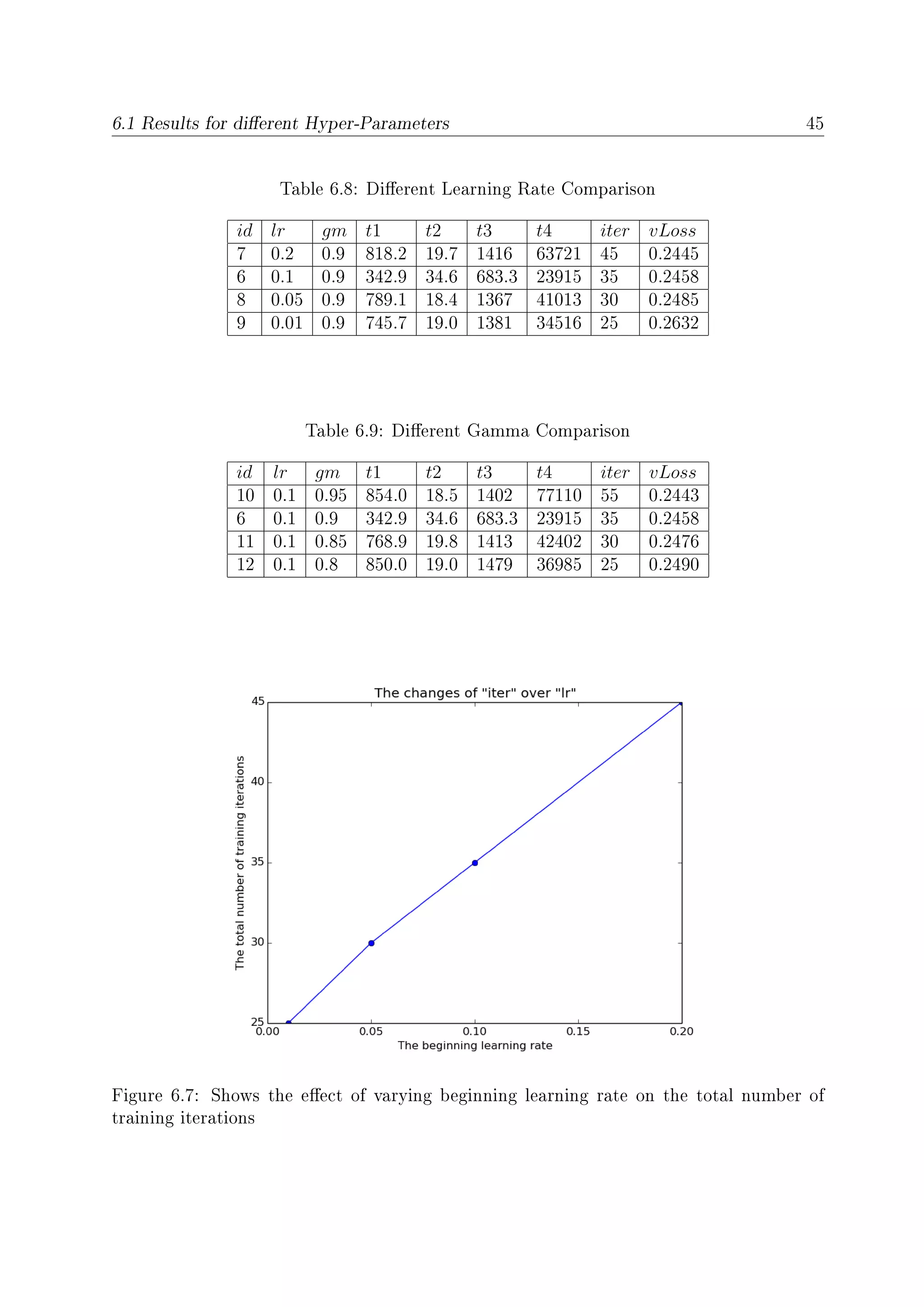
6.6 Shows the eect of varying beginning learning rate on the best loss of vali-
dation set . . . . . . . . . . . . . . . . . . . . . . . . . . . . . . . . . . . . 44
6.7 Shows the eect of varying beginning learning rate on the total number of
training iterations . . . . . . . . . . . . . . . . . . . . . . . . . . . . . . . . 45
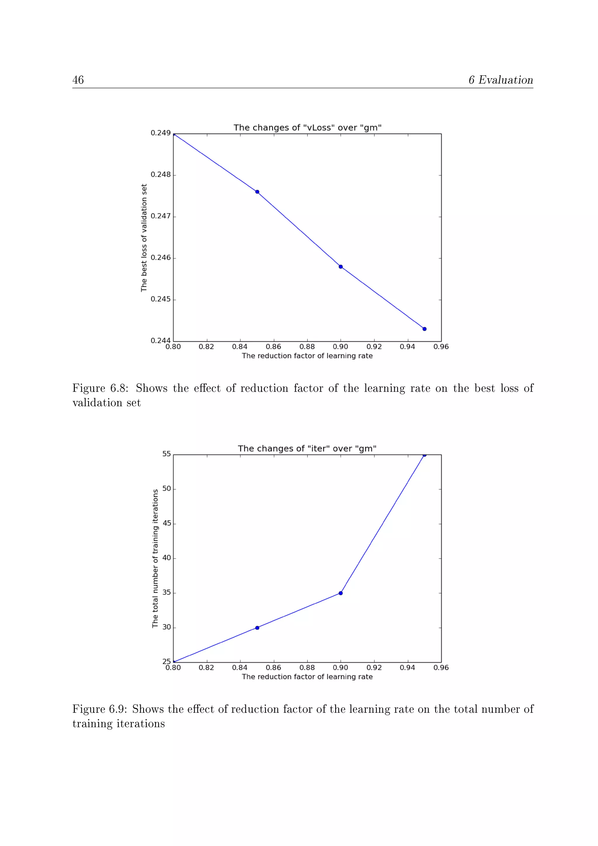
6.8 Shows the eect of reduction factor of the learning rate on the best loss of
validation set . . . . . . . . . . . . . . . . . . . . . . . . . . . . . . . . . . 46
6.9 Shows the eect of reduction factor of the learning rate on the total number
of training iterations . . . . . . . . . . . . . . . . . . . . . . . . . . . . . . 46
6.10 Nearest words from apple . . . . . . . . . . . . . . . . . . . . . . . . . . . 51
xi](https://image.slidesharecdn.com/eafda45f-0c51-4ed1-b9f3-f7670fd415ea-160726141620/75/HaiqingWang-MasterThesis-11-2048.jpg)

![Chapter 1
Introduction
1.1 Word Embedding
Machine learning approaches for natural language processing have to represent the words
of a language in a way such that Machine Learning modules may process them. This is
especially important for text mining, where data mining modules analyze text corpora to
extract their properties and semantics.
Consider a corpus C of interest containing documents and sentences. Traditional text
mining analyses use the vector space representation [Salton et al., 1975], where a word w
is represented by a sparse vector of the size N of the vocabulary D (usually N ≥ 100.000),
where all values are 0 except the entry for the actual word. This representation is also
called One-hot representation. This sparse representation, however, has no information on
the semantic similarity of words.
Recently word representations have been developed which represent each word w as a
real vector of d real numbers (e.g. d = 100) as proposed by [Collobert and Weston,
2008] and [Mikolov et al., 2013]. Generally, we call such a vector v(w) ∈ k
a word
embedding. By using a large corpus in an unsupervised algorithm word representations
may be derived such that words with similar syntax and semantics have representations
with a small Euclidean distance. Hence the distances between word embeddings correspond
to the semantic similarity of underlying words. These embeddings may be visualized to
show comunalities and dierences between words, sentences and documents. Subsequently
these word representations may be employed for further text mining analyses like opinion
mining [Socher et al., 2013], Kim 2014, Tang et al. 2014) or semantic role labeling [Zhou
and Xu, 2015] which benet from this type of representation [Collobert et al., 2011].
These algorithms are based on the very important assumption that if the contexts of two
words are similar, their meaning and therefore representations should be similar as well
[Harris, 1954]. Consider a sentence (or document) Si in the corpus C consisting of Li
words Si = (wi,1, wi,2, . . . , wi,Li
). Then the context of a word wt may be dened as the
1](https://image.slidesharecdn.com/eafda45f-0c51-4ed1-b9f3-f7670fd415ea-160726141620/75/HaiqingWang-MasterThesis-17-2048.jpg)
![2 1 Introduction
words in the neighborhood of wt in the sentence. Figure 1.1 shows how neighboring words
determine the sense of the word bank in a number of example sentences. So many actual
text mining methods make use of the context of words to generate embeddings.
Figure 1.1: Neigboring words dening the specic sense of bank.
Traditional word embedding methods rst obtain the co-occurrence matrix and then per-
form dimension reduction using singular value decomposition (SVD) [Deerwester et al.,
1990].
Recently, articial neural networks became very popular to generate word embeddings.
Prominent algorithms are Senna [Collobert and Weston, 2008], Word2vec [Mikolov et al.,
2013] and Glove [Pennington et al., 2014]. They all use randomly initialized vectors to
represent words. Subsequently these embeddings are modied in such a way that the word
embeddings of the neigboring words may be predicted with minimal error by a simple
neural network function.
1.2 Sense Embedding
Note that in the approaches described above each word is mapped to a single embedding
vector. It is well known, however, that a word may have several dierent meanings, i.e. is
polysemous. For example the word bank among others may designate:
• the slope beside a body of water,
• a nancial institution,
• a ight maneuver of an airplane.
Further examples of polysemy are the words book, milk or crane. WordNet [Fell-
baum, 1998] and other lexical resources show that most common words have 3 to 10
dierent meanings. Obviously each of these meanings should be represented by a separate](https://image.slidesharecdn.com/eafda45f-0c51-4ed1-b9f3-f7670fd415ea-160726141620/75/HaiqingWang-MasterThesis-18-2048.jpg)
![1.3 Goal 3
embedding vector, otherwise the embedding will no longer represent the underlying sense.
This in addition will harm the performance of subsequent text mining analyses. Therefore
we need methods to learn embeddings for senses rather than words.
Sense embeddings are a renement of word embeddings. For example, bank can appear
either together with money, account, check or in the context of river, water,
canoe. And the embeddings of the words money, account, check will be quite
dierent from the embeddings of river, water, canoe. Consider the following two
sentences
• They pulled the canoe up the bank.
• He cashed a check at the bank.
The word bank in the rst sentence has a dierent sense than the word bank in the
second sentence. Obviously, the context is dierent.
So if we have a methods to determine the dierence of the context, we can relabel the
word bank to the word senses bank1 or bank2 denoting the slope near a river or the
nancial institution respectively. We call the number after the word the sense labels of the
word bank. This process can be performed iteratively for each word in the corpus by
evaluating its context.
An alternative representation of words is generated by topic models [Blei et al., 2003],
which represent each word of a document as a nite mixture of topic vectors. The mixture
weights of a word depend on the actual document. This implies that a word gets dierent
representations depending on the context.
In the last years a number of approaches to derive sense embeddings have been presented.
Huang et al. [2012] used the clustering of precomputed one-sense word embeddings and
their neighborhood embeddings to dene the dierent word senses. The resulting word
senses are xed to the corresponding words in the sentences. Their embedding vectors
are trained until convergence. A similar approach is described by Chen et al. [2014].
Instead of a single embedding each word is represented by a number of dierent sense
embeddings. During each iteration of the supervised training, for each position of the
word, the best tting embedding is selected according the tness criterion. Subsequently
only this embedding is trained using back-propagation. Note that during training a word
may be assigned to dierent senses thus reecting the training process. A related approach
was proposed by Tian et al. [2014].
1.3 Goal
It turned out that the resulting embeddings get better with the size of the training corpus
and an increase of the dimension of the embedding vectors. This usually requires a parallel](https://image.slidesharecdn.com/eafda45f-0c51-4ed1-b9f3-f7670fd415ea-160726141620/75/HaiqingWang-MasterThesis-19-2048.jpg)
![4 1 Introduction
environment for the execution of the training of the embeddings. Recently Apache Spark
[Zaharia et al., 2010] has been presented, an opensource cluster computing framework.
Spark provides the facility to utilize entire clusters with implicit data parallelism and
fault-tolerance against resource problems, e.g. memory shortage. The currently available
sense embedding approaches are not ready to use compute clusters, e.g. by Apache Spark.
Our goal is to investigate sense assignment models which will extend known word em-
bedding (one sense) approaches and implement such method on a compute cluster using
Apache Spark to be able to process larger training corpora and employ higher-dimensional
sense embedding vectors. So that we can derive expressive word representations for dif-
ferent senses in an ecient way. And our main work will focus on the extension of the
Skip-gram model [Mikolov et al., 2013] in connection to the approach of [Neelakantan et al.,
2015] because these models are easy to use, very ecient and convenient to train.
1.4 Outline
The rest of the thesis is structured as the following. Chapter 2 introduces the background
about word embeddings and explains the mathematical details of one model (word2vec
Mikolov et al. [2013]) that one must be acquainted with in order to understand the work
presented. Chapter 3 presents some relevant literature and several latest approaches about
sense embedding. Chapter 4 describes the mathematical model of our work for sense
embedding. Chapter 5 introduces the Spark framework and discusses in detail the imple-
mentation of our model. Chapter 6 analyzes the eect of dierent parameters from the
model and compares the result with other models. Chapter 7 represents concluding re-
marks to our work including the advantages and disadvantages and talks about what can
be done further to improve our model.](https://image.slidesharecdn.com/eafda45f-0c51-4ed1-b9f3-f7670fd415ea-160726141620/75/HaiqingWang-MasterThesis-20-2048.jpg)
![Chapter 2
Background
2.1 Word Embedding
Recently machine learning algorithms are used often in many NLP tasks, but the machine
can not directly understand human language. So the rst thing is to transform the language
to the mathematical form like word vectors, that is using digital vectors to represent words
in natural languages. The above process is called word embedding.
One of the easiest word embeddings is using a one-hot representation, which uses a long
vector to represent a word. It only has one component which is 1, and the other components
are all 0s. The position of 1 corresponds to the index of the word in dictionary D. But
this word vector representation has some disadvantages, such as troubled by the huge
dimensionality |D|. Most important it can not describe the similarity between words well.
An alternative word embedding is the Distributed Representation. It was rstly proposed
by Williams and Hinton [1986] and can overcome the above drawbacks from one-hot rep-
resentation. The basic idea is to map each word into a short vector of xed length (here
short is with respect to long dimension |D| of the one-hot representation). All of these
vectors constitute a vector space, and each vector can be regarded as a point in the vector
space. After introducing the distancein this space , it is possible to judge the similarity
between words (morphology and syntax) according to the distance.
There are many dierent models which can be used to estimate a Distributed Represen-
tation vector, including the famous LSA (Latent Semantic Analysis) [Deerwester et al.,
1990] and the LDA (Latent Dirichlet Allocation) [Blei et al., 2003]. In addition, the neural
network algorithm based language model is a very common method and becomes more
and more popular. A language model has the task to predict the next word in a sentence
from the words observed so far. In these neural network based models, the main goal is
to generate a language model usually generating a word vectors as byproducts. In fact, in
most cases, the word vector and the language model are bundled together. The rst paper
on this is the Neural Probabilistic Language Model from [Bengio et al., 2003], followed by
5](https://image.slidesharecdn.com/eafda45f-0c51-4ed1-b9f3-f7670fd415ea-160726141620/75/HaiqingWang-MasterThesis-21-2048.jpg)
![6 2 Background
Figure 2.1: Graph of the tanh function
a series of related research, including SENNA from Collobert et al. [2011] and word2vec
from Mikolov et al. [2013].
Word embedding actually is very useful. For example, Ronan Collobert's team makes use
of the word vectors trained from software package SENNA ([Collobert et al., 2011]) to do
part-of-speech tagging, chunking into phrases, named entity recognition and semantic role
labeling, and achieves good results.
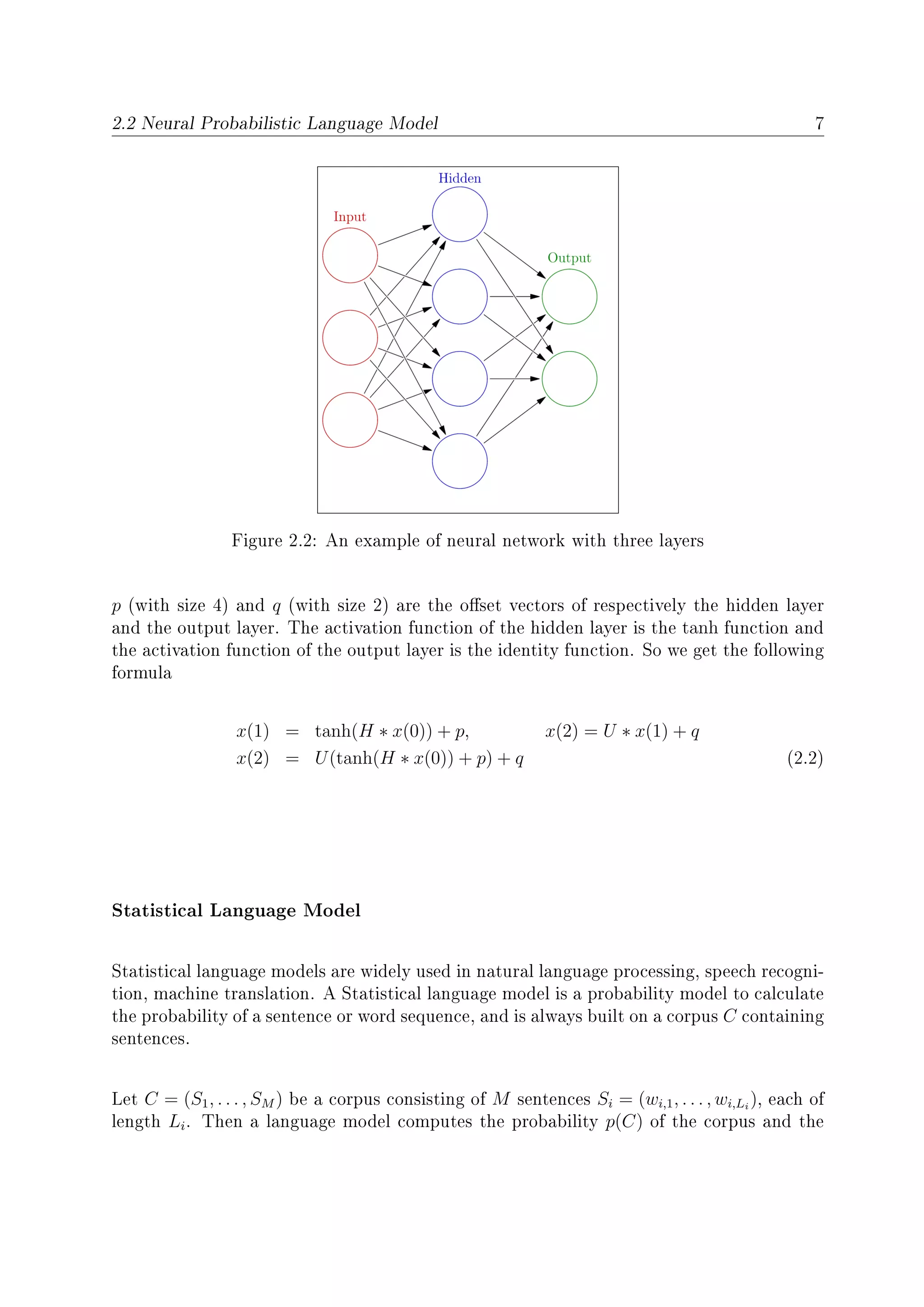
2.2 Neural Probabilistic Language Model
Neural Network
General speaking, a neural network denes a mapping between some input and output,
and it usually contains an input layer, an output layer and one or more hidden layers
between the input layer and the output layer. Each layer has some nodes meaning that it
can contains a vector with some dimension. Let x(i − 1) be the input vector to the i-th
layer and x(i) its output vector. From one layer to the next layer, there is a map function
f(x(i − 1)) = x(i) made up by an activation function with a weight matrix and and an
oset vector.
Specically vector x(i−1) is multiplied by a weight matrix H and then adds an oset vector
q, after that an activation function such as tanh function shown as Figure 2.1. Hence we
have
x(i) = f(x(i − 1)) = tanh(H ∗ x(i − 1)) + q (2.1)
Let's start with the simplest neural network with three layers (only one hidden layer) shown
as Figure 2.2. We can nd that input layer has three nodes, that is the input should be a
vector with dimension 3. The hidden layer has four nodes, which means the input vector
will be mapped to a hidden vector with dimension 4. And then it will be mapped again to
the output vector with dimension 2. Specically, the input is a vector x(0) (with dimension
3). H (with size 4 × 3) and U (with size 2 × 4) are respectively the weight matrix between
input layer and hidden layer and the weight matrix between hidden layer and output layer,](https://image.slidesharecdn.com/eafda45f-0c51-4ed1-b9f3-f7670fd415ea-160726141620/75/HaiqingWang-MasterThesis-22-2048.jpg)
![8 2 Background
probabilities p(Si) of the sentences Si according to the conditional probability denition
p(C) =
M
i=1
p(Si) (2.3)
p(Si) =
Li
t=1
p(wt|wt−1, . . . , w1)
≈
Li
t=1
p(wt|Prev(wt)) (2.4)
where Prevn−1
(wt) = (wi,max(t−n+1,1), . . . , wi,t) is the subsequence of n−1 past words before
wt in sentence Si. Note that the last equation is an approximation of the full conditional
probability. The core part of a Statistic language model is to compute p(wt|Prev(wt)) by
some model if Prev(wt) is given.
Neural Probabilistic Language Model
Bengio et al. [2003] introduce a neural probabilistic language model shown as Figure 2.3,
which uses neural network to approximate p(wt|Prev(wt)) the language model (2.4).
C is the given corpus containing the sentences/documents of words from a dictionary D.
Consider a word wt in some sentence Si = (w1, w2, . . . , wT−1, wLi
) of corpus C, where t is
some position in S and Li is the length of S. Let Prevn−1
(wt) = (wmax(t−n+1,1), . . . , wt−1)
be the subsequence of words before wt.
Firstly for each word w in dictionary D, there is a look-up table V mapping the word w to
vector V (w). Note that V is denoted as C in gure 2.3. The vector size of V (w) is d. The
input layer is a long vector concatenated by n − 1 word vectors in Prevn−1
(wt). So the
input vector is x with dimension (n − 1)d, and the output vector is y with the dimension
|D|, where D is vocabulary and |D| is the size of vocabulary.
Bengio et al. [2003] also use tanh function for the activation function in the hidden layer.
H (with size m × (n − 1)d) and U (with size |D| × m) are respectively the weight matrix
between input layer and hidden layer and the weight matrix between hidden layer and
output layer, p (with size m)and q (with size D) are the oset vectors of respectively the
hidden layer and the output layer. Additionally, they introduce another weight matrix
between the input layer and output layer W (with size |D| × (n − 1)d). So the mapping
function from x to the output is
y = q + U ∗ tanh(p + H ∗ x) + W ∗ x (2.5)](https://image.slidesharecdn.com/eafda45f-0c51-4ed1-b9f3-f7670fd415ea-160726141620/75/HaiqingWang-MasterThesis-24-2048.jpg)
![2.2 Neural Probabilistic Language Model 9
Figure 2.3: The neural network structure from [Bengio et al., 2003]
Softmax Function
The softmax function, is a generalization of the logistic function that squashes a K-
dimensional vector z of arbitrary real values to a K-dimensional vector σ(z) of real values
in the range (0, 1) that add up to 1
1
. The function is given by
σ(z)j =
ezj
K
k=1 ezk
for j = 1, . . . , K.
From above, we know the output y is a vector with the length of |D| with arbitrary values
and can not represent probabilities. Because it is a language model, it needs to model the
probability as p(wt|Prevn−1
(wt)). Actually, Bengio et al. [2003] use the softmax function
to do normalization. After normalization, the nal result is a value between 0 to 1, which
can represent a probability. Using xwt to represent the input vector connected by word
vectors from Context(wt) and ywt to represent the output vector mapped from the neural
network. From Formula 2.5 we have
ywt = q + U ∗ tanh(p + H ∗ xwt ) + W ∗ xwt (2.6)
1https://en.wikipedia.org/wiki/Softmax_function](https://image.slidesharecdn.com/eafda45f-0c51-4ed1-b9f3-f7670fd415ea-160726141620/75/HaiqingWang-MasterThesis-25-2048.jpg)
![10 2 Background
and p(wt|Prevn−1
(wt)) can be expressed as
p(wt|Prevn−1
(wt)) =
eywt,iwt
|D|
i=1 eywt,i
, (2.7)
where iwt represents the index of wt in the dictionary D, ywt,i means the i-th element in
the vector ywt . Note that the denominator contains a term eywt,i
for every word in the
vocabulary. The goal is also to maximize the function shown as 2.4. In the beginning, all
word vectors are initialized randomly. And after maximizing the objective function, they
can get the meaningful word vectors.
2.3 The model of Collobert and Weston
The main purpose of the approach of Collobert and Weston [2008] originally is not to build
a language model, but to use the word vectors from their model to complete several tasks
from natural language processing, such as speech tagging, named entity recognition, phrase
recognition, semantic role labeling, and so on ([Collobert and Weston, 2008] and [Collobert
et al., 2011]). Due to the dierent purpose, their training method is also dierent. They
do not use the Formula 2.4 as other language models used. Their idea is to optimize a
score function on phrase so that if the phrase is reasonable or makes sense, the score would
be positive, otherwise the score would be negative.
C is the given corpus with a vocabulary D of size N. Consider a word wt in some sentence
S = (w1, w2, . . . , wT−1, wT ) from corpus C, where t is some position of S and T is the
length of S. Dene phrase(wt) = (wt−c, . . . , wt−1, wt, wt+1, . . . , wt+c), and c is the number
of words before and after wt. Note that phrase(wt) contains wt. We dene phrase(wt) as
phrase(wt) where the center word wt is replaced by anther random word w = wt. Each
word is represented by a vector of dimension d . For phrase phrase(wt), connect these 2c+1
vectors to be a long vector xwt with dimension d × (2c + 1). The input of f is the vector
xwt with dimension d × (2c + 1). And the output is a real number (positive or negative).
Use xwt
to represent the vector connected by 2c + 1 word vectors from phrase(wt) .
[Collobert and Weston, 2008] also use a neural network to build their model. But the neural
network structure is dierent from the network structure in [Bengio et al., 2003]. Its output
layer has only one node representing the score, rather than Bengio's N nodes, where N is
the size of dictionary D. Note that Bengio's model uses another softmax funtion to get
the probability value in order to represent the Formula 2.7. Doing so greatly reduced the
computational complexity.
Based on the above description, the model use f to represent its neural network, the input
is a phrase vector, the output can be an arbitrary real number. Note that there is no
active function in the output layer. The objective of this model is that for every phrase](https://image.slidesharecdn.com/eafda45f-0c51-4ed1-b9f3-f7670fd415ea-160726141620/75/HaiqingWang-MasterThesis-26-2048.jpg)
![12 2 Background
Figure 2.4: word2vec
samples is K. And P(w) is the smoothed unigram distribution which is used to generate
negative samples. Specically for each w ∈ D
P(w) =
count(w)
3
4
( M
i=1 Li)
3
4
where count(w) is the number of times w occurred in C and
M
i=1 Li is the number of
total words in C. The objective function of skip-gram model with negative sampling can
be dened specically as
G =
1
M
M
i=1
1
Li
Li
t=1 −c ≤ j ≤ c
j = 0
1 ≤ j + t ≤ Li
log p(wi,t+j|wi,t) +
K
k=1
Ezk∼P(w)log [1 − p(zk|wi,t)]
(2.10)
where p(w |w) = σ(Uw
T
Vw) and σ(x) = 1
1+e−x .
p(wi,t+j|wi,t) is the probability of using center word wi,t to predict one surrounding word
wi,t+j, which needs to be maximized. z1,. . . ,zK are the negative sample words to replace
word wi,t+j, and p(zk|wi,t) (1 ≤ k ≤ K) is the probability of using center word wi,t to](https://image.slidesharecdn.com/eafda45f-0c51-4ed1-b9f3-f7670fd415ea-160726141620/75/HaiqingWang-MasterThesis-28-2048.jpg)
![2.4 Word2Vec 13
predict one negative sample word zk, which needs to be minimized. Equivalently, the
whole objective function needs to be maximized.
Take the word pair (wi,t, wi,t+j) as a training sample, and dene loss function loss for
each sample
loss(wi,t, wi,t+j) = −log p(wi,t+j|wi,t) −
K
k=1
Ezk∼P(w)log [1 − p(zk|wi,t)] (2.11)
Here the loss is dened as the negative log probability of wi,t given wi,t+j.
And the loss function of whole corpus is
loss(C) =
1
M
M
i=1
1
Li
Li
t=1 −c ≤ j ≤ c
j = 0
1 ≤ j + t ≤ Li
loss(wi,t, wi,t+j)
To maximize the objective function is equivalently to minimize the loss function. So the
objective of learning algorithm is
arg min
{V,U}
1
M
M
i=1
1
Li
Li
t=1 −c ≤ j ≤ c
j = 0
1 ≤ j + t ≤ Li
loss(wi,t, wi,t+j)
Use
It =
1
M
M
i=1
1
Li
Li
t=1 −c ≤ j ≤ c
j = 0
1 ≤ j + t ≤ Li
1
to represent the number of total training samples in one epoch. (An epoch is a measure of
the number of times all of the training samples are used once.) And the number of epochs
is T. So the total iterations is It ∗ T.
Use stochastic gradient descent:
2
• Initialize {V, U}
• For It ∗ T Iterations:
For each training sample (wi,t, wi,t+j)
∗ Generate negative sample words to replace wi,t+j: (w1, . . . , zk)
2https://en.wikipedia.org/wiki/Stochastic_gradient_descent](https://image.slidesharecdn.com/eafda45f-0c51-4ed1-b9f3-f7670fd415ea-160726141620/75/HaiqingWang-MasterThesis-29-2048.jpg)
![14 2 Background
∗ Calculate the gradient ∆ = − {V,U}loss(wi,t, wi,t+j)
∗ ∆ is only made up by {∆Vwi,t
, ∆Uwi,t+j
, [∆Uw1
, . . . , ∆Uzk
]}
∗ Update Embeddings:
· Vwi,t
= Vwi,t
+ α∆Vwi,t
· Uwi,t+j
= Uwi,t+j
+ α∆Uwi,t+j
· Uzk
= Uzk
+ α∆Uzk
, 1 ≤ k ≤ K
(α is the learning rate and will be updated every several iterations)
The detail of gradient calculation of loss(wi,t, wi,t+j) is
∆Vwi,t
= −
∂loss(wi,t, wi,t+j)
∂Vwi,t
= [1 − log σ(UT
wi,t+j
Vwi,t
)]Uwi,t+j
+
k
i=1
[−log σ(UT
zk
Vwi,t
))]Uzk
∆Uwi,t+j
= −
∂loss(wi,t, wi,t+j)
∂Uwi,t+j
= [1 − log σ(UT
wi,t+j
Vwi,t
)]Vwi,t
∆Uzk
= −
∂loss(wi,t, wi,t+j)
∂Uzk
= [−log σ(UT
zk
Vwi,t
))]Vwi,t
, 1 ≤ k ≤ K](https://image.slidesharecdn.com/eafda45f-0c51-4ed1-b9f3-f7670fd415ea-160726141620/75/HaiqingWang-MasterThesis-30-2048.jpg)
![Chapter 3
Related Works
3.1 Huang's Model
The work of Huang et al. [2012] is based on the model of Collobert and Weston [2008].
They try to make embedding vectors with richer semantic information. They had two major
innovations to accomplish this goal : The rst innovation is using global information from
the whole text to assist local information, the second innovation is using the multiple word
vectors to represent polysemy.
Huang thinks Collobert and Weston [2008] use only local context. In the process of
training vectors, they used only 10 words as the context for each word, counting the center
word itself, there are totally 11 words' information. This local information can not fully
exploit the semantic information of the center word. Huang used their neural network
directly to compute a score as the local score.
And then Huang proposed a global information, which is somewhat similar to the tra-
ditional bag of words model. Bag of words is about accumulating One-hot Representation
from all the words of the article together to form a vector (like all the words thrown in a
bag), which is used to represent the article. Huang's global information used the average
weighted vectors from all words in the article (weight is word's idf), which is considered
the semantic of the article. He connected such semantic vector of the article (global in-
formation) with the current word's vector (local information) to form a new vector with
double size as an input, and then used the CW's network to calculate the score. Figure
[huang] shows such structure. With the local score from original CW approach and
Global score from improving method based on the CW approach, Huang directly add
two scores as the nal score. The nal score would be optimized by the pair-wise target
function from CW. Huang found his model can capture better semantic information.
The second contribution of this paper is to represent polysemy using multiple embeddings
for a single word. For each center word, he took 10 nearest context words and calculated the
15](https://image.slidesharecdn.com/eafda45f-0c51-4ed1-b9f3-f7670fd415ea-160726141620/75/HaiqingWang-MasterThesis-31-2048.jpg)
![16 3 Related Works
Figure 3.1: The network structure from [Huang et al., 2012]
Table 3.1: Senses computed with Huang's network and their nearest neighbors.
Center Word Nearest Neighbors
bank_1 corporation, insurance, company
bank_2 shore, coast, direction
star_1 movie, lm, radio
star_2 galaxy, planet, moon
cell_1 telephone, smart, phone
cell_2 pathology, molecular, physiology
left_1 close, leave, live
left_2 top, round, right
weighted average of the embeddings of these 10 word vectors (idf weights) as the context
vector. Huang used all context vectors to do a k-means clustering. He relabel each word
based on the clustering results (dierent classes of the same words would be considered as
dierent words to process). Finally he re-trained the word vectors. Table 3.1 gives some
examples from his model's results.
3.2 EM-Algorithm based method
Tian et al. [2014] proposed an approach based on the EM-algorithm from . This method
is the extension of the normal skip-gram model. They still use each center word to predict
several context words. The dierence is that each center word can have several senses
with dierent probabilities. The probability should represent the relative frequency of the
sense in the corpus. For example, considering bank1 in the sense of side of the river and
bank2 meaning nancial institution. Usually bank1 will have a smaller probability and](https://image.slidesharecdn.com/eafda45f-0c51-4ed1-b9f3-f7670fd415ea-160726141620/75/HaiqingWang-MasterThesis-32-2048.jpg)
![3.2 EM-Algorithm based method 17
Table 3.2: Word senses computed by Tian et al.
word Prior Probability Most Similar Words
apple_1 0.82 strawberry, cherry, blueberry
apple_2 0.17 iphone, macintosh, microsoft
bank_1 0.15 river, canal, waterway
bank_2 0.6 citibank , jpmorgan, bancorp
bank_3 0.25 stock, exchange, banking
cell_1 0.09 phones cellphones, mobile
cell_2 0.81 protein, tissues, lysis
cell_3 0.01 locked , escape , handcued
bank2. We can say in the corpus, in most sentences of the corpus the word bank means
nancial institution and in other fewer cases it means side of the river.
Objective Function
Considering wI as the input word and wO as the output word, (wI, wO) is a data sample.
The input word wI have NwI
prototypes, and it appears in its hwI
-th prototype, i.e.,
hwI
∈ {1, .., NwI
} [] The prediction P(wO|wI) is like the following formula
p(wO|wI) =
NwI
i=1
P(wO|hwI
= i, wI)P(hwI
= i|wI) =
NwI
i=1
exp(UT
wO
VwI ,i)
w∈Wexp(UT
w VwI ,i)
P(hwI
= i|wI)
where VwI ,i ∈ Rd
refers to the d-dimensional input embedding vector of wI's i-th proto-
type and UwO
∈ Rd
represents the output embedding vectors of wO. Specically, they
use the Hierarchical Softmax Tree function to approximate the probability calculation.
Algorithm Description
Particularly for the input word w, they put all samples (w as the input word) together like
{(w, w1), (w, w2), (w, w3)...(w, wn)} as a group. Each group is based on the input word. So
the whole training set can be separated as several groups. For the group mentioned above,
one can assume the input word w has m vectors (m senses), each with the probability
pj(1 ≤ j ≤ m). And each output word wi(1 ≤ i ≤ n) has only one vector.
In the training process, for each iteration, they fetch only part of the whole training set
and then split it into several groups based on the input word. In each E-step, for the group
mentioned above, they used soft label yi,j to represent the probability of input word in
sample (w, wi) assigned to the j-th sense. The calculating of yi,j is based on the value of
sense probability and sense vectors. After calculating each yi,j in each data group, in the
M-step, they use yi,j to update sense probabilities and sense vectors from input word, and
the word vectors from output word. Table 3.2 lists some results from this model.](https://image.slidesharecdn.com/eafda45f-0c51-4ed1-b9f3-f7670fd415ea-160726141620/75/HaiqingWang-MasterThesis-33-2048.jpg)
![18 3 Related Works
3.3 A Method to Determine the Number of Senses
Neelakantan et al. [2015] comes up with two dierent models, the rst one is the MSSG
(Multi-Sense Skip-gram) model, in which the number of senses for each word is xed and
decided manually. The second one is NP-MSSG (Non-Parametric MSSG) which is based
on the MSSG model , the number of senses for each word in this model is not xed and
can be decided dynamically by the model itself.
MSSG
C is the given corpus containing the sentences/documents of words. N is the number of
dierent words in the corpus C. D is the vocabulary (the set of N dierent words in
the corpus C). Considering a word wt in some sentence S = (w1, w2, . . . , wT−1, wT ) from
corpus C, where t is some position of S and T is the length of S, dene Context(w) =
(w,max(t−c,1), . . . , wt−1, wt+1, . . . , w,min(t+c,T)), and c is the number of words before and after
wt in the Context(w).
In the MSSG model, each word has S senses (S is set advance manually. Like huang's
model, MSSG model uses the clustering, but its clustering strategy is dierent. Assuming
each word has a context vector, which is summed up by all word vectors in the context.
Huang's model do clustering on all context vectors (calculated by the weighted average of
word vectors) from the corpus. While for MSSG model, they do clustering based on each
word, that is each word has its own context clusters. Another thing is that MSSG only
records the information (vector) of context cluster center for each word. For example, word
w has S clusters , it has only S context vectors. And in the initialization, these S context
vectors are set randomly. When there is a new context of word w, the model will rstly
check which cluster this context should belong to and then use this new context vector to
update the vector of selected context cluster center.
Specically, each word has a global vector, S sense vectors and S context cluster center
vectors. All of them are initialized randomly. For word wt, its global vector is vg(wt)
and its context vectors are vg(wt−c), . . . , vg(wt−1), vg(wt+1), . . . , vg(wt+c). vcontext(ct) is the
average context vector calculated by the average of these 2c global word vectors. And
wt's sense vectors are vs(wt, s)(s = 1, 2, . . . , S) and the context cluster center vectors are
µ(wt, s)(s = 1, 2, . . . , S). The architecture of the MSSG is like Figure 3.2 when c = 2. It
uses the following formula to select the best cluster center:
st = arg max
s=1,2,...,S
sim(µ(wt, s), vcontext(ct))
where st is index of selected cluster center and sim is the cosine similarity function. The
selected context cluster center vector µ(wt, st) will be updated with current context vector
vcontext(ct). And then the model selects v(w, st) as current word's sense. The rest thing
is similar as skip-gram model: use this sense vector to predict global word vectors in the
context and then update these global word vectors and this sense vector.](https://image.slidesharecdn.com/eafda45f-0c51-4ed1-b9f3-f7670fd415ea-160726141620/75/HaiqingWang-MasterThesis-34-2048.jpg)


![Chapter 4
Solution
In this section we present a model for the automatic generation of embeddings for the
dierent senses of words. Generally speaking, our model is a extension of skip-gram model
with negative sampling. We assume each word in the sentence can have one or more senses.
As described above Huang et al. [2012] cluster the embeddings of word contexts to label
word senses and once assigned, these senses can not be changed. Our model is dierent.
We do not assign senses to words in a preparatory step, instead we just initialize each
word with random senses and they can be adjusted afterwards. We also follow the idea
from EM-Algorithm based method [Tian et al., 2014], word's dierent senses have dierent
probabilities, the probability can represent if a sense is used frequent in the corpus.
In fact, after some experiments, we found our original model is not good. So we simplied
our original model. Anyhow we will introduce our original model and show the failures in
the next chapter, and explain the simplication.
4.1 Denition
C is the corpus containing M sentences, like (S1, S2, . . . , SM ), and each sentence is made
up by several words like Si = (wi,1, wi,2, . . . , wi,Li
) where Li is the length of sentence Si.
We use wi,j ∈ D to represent the word token from the vocabulary D in the position j of
sentence Si. We assume that each word w ∈ D in each sentence has Nw ≥ 1 senses. We
use the lookup function h to assign senses to words in a sentence, specically hi,j is the
sense index of word wi,j (1 ≤ hi,j ≤ Nwi,j
).
Similar to Mikolov et al. [2013] we use two dierent embeddings for the input and the
output of the network. Let V and U to represent respectively the set of input embedding
vectors and the set of output embedding vectors respectively. And each embedding vectors
has the dimension d. Additionally, Vw,s ∈ d
means the input embedding vectors from
sense s of word w. Similarly Uw,s ∈ d
is the ouput embedding of word w where w ∈ D,
1 ≤ s ≤ Nw. Following the Skip-gram model with negative sampling, K. The context of a
21](https://image.slidesharecdn.com/eafda45f-0c51-4ed1-b9f3-f7670fd415ea-160726141620/75/HaiqingWang-MasterThesis-37-2048.jpg)
![22 4 Solution
word wt in the sentence Si may be dened as the subsequence of the words Context(wt) =
(wi,max(t−c,0), . . . , wi,t−1, wi,t+1, . . . , wi,min(t+c,Li)), where c is the size of context. And P(w) is
the smoothed unigram distribution which is used to generate negative samples. Specically,
P(w) = count(w)
3
4
( M
i=1 Li)
3
4
(w ∈ D), where count(w) is the number of times w occurred in C and
M
i=1 Li is the number of total words in C.
4.2 Objective Function
Based on the skip-gram model with negative sampling. We still use same neural network
structure to optimize the probability of using the center word to predict all words in the
context. The dierence is that, such probability is not about word prediction, instead
it is about sense prediction. We use (w, s) to represent the word w's s-th sense, i.e.
(wi,t, hi,t) represents the word wi,t's hi,t-th sense, and p((wi,t+j, hi,t+j)|(wi,t, hi,t)) represents
the probability using wi,t's hi,t-th sense to predict wi,t+j's hi,t+j-th sense, where wi,t and
wi,t+j are indexes of words in the position t and t + j respectively from sentence Si. And
hi,t and hi,t+j represent their assigned sense indexes, which can be adjusted by model
in the training. The above prediction probability is only for a pair of word with sense
information, the goal of the model is to maximize every possible pairs of words which can
use a probability computed by producing every prediction probabilities of word pairs to
resent the prediction probability based on the whole corpus. The model's task is to adjust
sense assignment and learn sense vectors in order to get the biggest prediction probability
based on the whole corpus. Specically, we use the following likelihood function to achieve
above objective
G =
1
M
M
i=1
1
Li
Li
t=1 −c ≤ j ≤ c
j = 0
1 ≤ j + t ≤ Li
log p (wi,t+j, hi,t+j)|(wi,t, hi,t)
+
K
k=1
Ezk∼Pn(w)log 1 − p [zk, R(Nzk
)]|(wi,t, hi,t)
(4.1)
where p (w , s )|(w, s) = σ(Uw ,s
T
Vw,s) and σ(x) = 1
1+e−x .
p (wi,t+j, hi,t+j)|(wi,t, hi,t) is the probability of using center word wi,t with sense hi,t to
predict one surrounding word wi,t+j with sense hi,t+j, which needs to be maximized.
[z1, R(Nz1 )],. . . ,[(zK, R(NzK
)] are the negative sample words with random assigned senses
to replace (wi,t+j, hi,t+j), and p [zk, R(Nzk
)]|(wi,t, hi,t) (1 ≤ k ≤ K) is the probability of
using center word wi,t with sense hi,t to predict one negative sample word zk with sense](https://image.slidesharecdn.com/eafda45f-0c51-4ed1-b9f3-f7670fd415ea-160726141620/75/HaiqingWang-MasterThesis-38-2048.jpg)
![4.2 Objective Function 23
R(Nzk
), which needs to be minimized. It is noteworthy that, hi,t (wi,t's sense) and hi,t+j
(wi,t+j's sense) are assigned advance and hi,t may be changed in the Assign. But zk's sense
sk is always assigned randomly.
The nal objective is to nd out optimized parameters θ = {h, U, V } to maximize the
Objective Function G, where h is updated in the Assign and {U, V } is updated in the
Learn.
In the Assign, we use score function fi,t with xed negative samples
∪
−c ≤ j ≤ c
j = 0
1 ≤ j + t ≤ Li
[(zj,1, sj,1), . . . , (zj,K, sj,K)] (senses are assigned randomly already)
fi,t(s) =
−c ≤ j ≤ c
j = 0
1 ≤ t + j ≤ Li
log p[(wi,t+j, hi,t+j)|(wi,t, s)] +
K
k=1
log 1 − p[(zj,k, sj,k)|(wi,t, s)]
to select the best sense (with the max value) for word wi,t. In the Learn, we take
[(wi,t, hi,t), (wi,t+j, hi,t+j)] as a training sample and use the negative log probability as loss
function loss for each sample
loss (wi,t, hi,t), (wi,t+j, hi,t+j)
= −log p (wi,t+j, hi,t+j)|(wi,t, hi,t) −
K
k=1
Ezk∼Pn(w)log 1 − p [zk, R(Nzk
)]|(wi,t, hi,t)
And the loss function of whole corpus is
loss(C) =
1
M
M
i=1
1
Li
Li
t=1 −c ≤ j ≤ c
j = 0
1 ≤ j + t ≤ Li
loss (wi,t, hi,t), (wi,t+j, hi,t+j)
After Assign, h is xed. So we the same method in the normal Skip-gram with negative
sampling model (stochastic gradient decent) to minimize G in the Learn. So the objective
of Learn is to get
arg min
{V,U}
1
M
M
i=1
1
Li
Li
t=1 −c ≤ j ≤ c
j = 0
1 ≤ j + t ≤ Li
loss (wi,t, hi,t), (wi,t+j, hi,t+j)](https://image.slidesharecdn.com/eafda45f-0c51-4ed1-b9f3-f7670fd415ea-160726141620/75/HaiqingWang-MasterThesis-39-2048.jpg)
![4.3 Algorithm Description 25
be ignored in the next iterations. Actually, we already did some experiments without sense
probabilities and these experiments' results really told use the above situation.
Next, we will describe the specic steps of Assign and Learn in the form of pseudo-code.
procedure Assign
for i:= 1 TO M do Loop over sentences.
repeat
for t:= 1 TO Li do Loop over words.
hi,t = max
1≤s≤Nwi,t
fi,t(s)
end for
until no hi,t changed
end for
end procedure
procedure Learn
for i:= 1 TO M do Loop over sentences.
for t:= 1 TO Li do Loop over words.
for FOR j:= −c TO c do
if j = 0 and t + j ≥ 1 and t + j ≤ Li then
generate negative samples (z1, s1), . . . , (zK, sK)
∆ = − θloss (wi,t, hi,t), (wi,t+j, hi,t+j)
∆ is made up by {∆Vwi,t,hi,t
, ∆Uwi,t+j,hi,t+j
, [∆Uw1,w1
, . . . , ∆Uzk,zk
]}
Vwi,t,hi,t
= Vwi,t,hi,t
+ α∆Vwi,t,hi,t
Uwi,t+j,hi,t+j
= Uwi,t+j,hi,t+j
+ α∆Uwi,t+j,hi,t+j
Uzk,sk
= Uzk,sk
+ α∆Uzk,sk
, 1 ≤ k ≤ K
end if
end for
end for
end for
end procedure
The detail of gradient calculation of loss (wi,t, hi,t), (wi,t+j, hi,t+j) is
∆Vwi,t,hi,t
= −
∂loss (wi,t, hi,t), (wi,t+j, hi,t+j)
∂Vwi,t,hi,t](https://image.slidesharecdn.com/eafda45f-0c51-4ed1-b9f3-f7670fd415ea-160726141620/75/HaiqingWang-MasterThesis-41-2048.jpg)
![26 4 Solution
= [1 − log σ(Uwi,t+j,hi,t+j
T
Vwi,t,hi,t
)]Uwi,t+j,hi,t+j
+
K
k=1
[−log σ(Uzk,sk
T
Vwi,t,hi,t
))]Uzk,sk
∆Uwi,t+j,hi,t+j
= −
∂loss (wi,t, hi,t), (wi,t+j, hi,t+j)
∂Uwi,t+j,hi,t+j
= [1 − log σ(Uwi,t+j,hi,t+j
T
Vwi,t,hi,t
)]Vwi,t,hi,t
∆Uzk,sk
= −
∂loss (wi,t, hi,t), (wi,t+j, hi,t+j)
∂Uzk,sk
= [−log σ(Uzk,sk
T
Vwi,t,hi,t
))]Vwi,t,hi,t
Iterating between Assign and Learn till the convergence of the value of G makes the
whole algorithm complete. Actually, we use the loss of validation set to monitor if the
training process is convergence. After a couple of iterations, we do the similar Assign
operation on validation set and then calculate the loss. To be noted that, the Assign on
validation set is a little dierent from the one on training set. Here, the negative samples
needs to be always xed throughout the training process. Another thing is that validation
set and training set should not be overlapped. As long as the validation loss begin to
increase. We stop training. And select the result with best validation loss as the nal
result.](https://image.slidesharecdn.com/eafda45f-0c51-4ed1-b9f3-f7670fd415ea-160726141620/75/HaiqingWang-MasterThesis-42-2048.jpg)
![Chapter 5
Implementation
For the implementation of our algorithm, we use the distributed framework Apache Spark
1
.
In this chapter, we will rstly introduce some knowledge about spark and how we use these
techniques to implement our model. After that, we will introduce the experiments we did
and analysis our results.
5.1 Introduction of Spark
Spark was developed by Zaharia et al. [2010] and has many useful features for the parallel
execution of programs. As the basic datastructure it has the RDD (Resilient Distributed
Dataset). The RDD is a special data structure containing the items of a dataset, e.g.
sentences or documents. Spark automatically distributes these items over a cluster of
compute nodes and manages its physical storage.
Spark has one driver and several executors. Usually, an executor is a cpu core, and we call
each machine as worker, so each worker has several executors. But logically we only need
the driver and the executors, only for something about tuning we should care about the
worker stu, e.g. some operations need to do communication between dierent machines.
But for most of cases, each executor just fetches part of data and deals with it, and then
the driver collects data from all executors.
The Spark operations can be called from dierent programming languages, e.g. Python,
Scala, Java, and R. For this thesis we use Scala to control the execution of Spark and to
dene its operations.
Firstly, Spark reads text le from le system (e.g. from the unix le system or from
HDFS, the Hadoop le system) and creates an RDD. An RDD usually is located in the
RAM storage of the dierent executors, but it may also stored on (persisted to) disks of
the executors. Spark operations follow the functional programming approach. There are
1http://spark.apache.org/
27](https://image.slidesharecdn.com/eafda45f-0c51-4ed1-b9f3-f7670fd415ea-160726141620/75/HaiqingWang-MasterThesis-43-2048.jpg)
![28 5 Implementation
two types of operations on RDDs: Transformation operations and action operations. A
transformation operation transforms a RDD to another RDD. Examples of transformation
operations are map (apply a function to all RDD elements), lter (select a subset of RDD
elements by some criterion), or sort (sort the RDD items by some key). Note that an RDD
is not mutable, i.e. cannot be changed. If its element are changed a new RDD is created.
Generally after some transformation operations, people use action operations to gain some
useful information from the RDD. Examples of action operations are count (count the
number of items), reduce (apply a single summation-like function), aggregate (apply several
summation-like functions), and collect (convert an RDD to a local array).
5.2 Implementation
We use syn0 to represent the input embedding V and syn1 to represent the output em-
bedding U. syn0 and syn1 are dened as broadcast variables, which are only readable and
can not be changed by executors. When they are changed in a training step copies are
returned as a new RDD.
Gradient Checking
Firstly we set a very small dataset mutually and calculate empirical derivative computed by
the nite dierence approaximation derivatives and the derivative computed as our model
shows from last chapter. The result shows the dierence between these two derivative is
very small. So our gradient calculation is correct.
Data preparing
We use the same corpus as other papers used, a snapshot of Wikipedia at April, 2010
created by Shaoul [2010], which has 990 million tokens. Firstly we count the all words
in the corpus. We transform all words to lower capital and then generate our vocabulary
(dictionary). And then we calculate the frequency of word count. For example, there
are 300 words which appear 10 times in the corpus. So the frequency of count 10 is
300. From this we can calculate the accumulated frequency. That is, if the accumulated
frequency of count 200 is 100000, there would be 100000 words whose count is at least 200.
This accumulated frequency can be used to select a vocabulary with the desired number of
entries, which all appear more frequent than c1 times in the corpus, where c1 is the minimal
count for the inclusion of a word in vocabulary D. The following 4 gures (Figure 5.1,Figure
5.2,Figure 5.3 and Figure 5.4) show the relationship between accumulated frequency and
word count. To make visualization more clear, we display it as four dierent gures with
dierent ranges of word count. And with some experience from other papers ([Huang et al.,
2012], [Tian et al., 2014] and [Neelakantan et al., 2015]), in some of our experiments we
set c1 = 20 and others have c1 = 200. Actually, when word count is 20, the accumulated](https://image.slidesharecdn.com/eafda45f-0c51-4ed1-b9f3-f7670fd415ea-160726141620/75/HaiqingWang-MasterThesis-44-2048.jpg)
![30 5 Implementation
Figure 5.1: Shows the accumulated frequency of word count in range [1,51]
Figure 5.2: Shows the accumulated frequency of word count in range [51,637]](https://image.slidesharecdn.com/eafda45f-0c51-4ed1-b9f3-f7670fd415ea-160726141620/75/HaiqingWang-MasterThesis-46-2048.jpg)
![5.2 Implementation 31
Figure 5.3: Shows the accumulated frequency of word count in range [637,31140]
Figure 5.4: Shows the accumulated frequency of word count in range [31140,919787]](https://image.slidesharecdn.com/eafda45f-0c51-4ed1-b9f3-f7670fd415ea-160726141620/75/HaiqingWang-MasterThesis-47-2048.jpg)

![Chapter 6
Evaluation
In the following chapter we use three dierent methods to evaluate our results. First we
compute the nearest neighbors of dierent word senses. Then we use the t-SNE approach to
project the embedding vectors to two dimensions and visualize semantic similarity. Finally
we perform the WordSim-353 task proposed by Finkelstein et al. [2001] and the Contextual
Word Similarity (SCWS) task from Huang et al. [2012].
The WordSim-353 dataset is made up by 353 pairs of words followed by similarity scores
from 10 dierent people and an average similarity score. The SCWS Dataset has 2003
words pairs with their context respectively, which also contains 10 scores from 10 dierent
people and an average similarity score. The task is to reproduce these similarity scores.
For the WordSim-353 dataset, we use the avgSim function to calculate the similarity of
two words w, ˜w ∈ D from our model as following
avgSim(w, ˜w) =
1
Nw
1
N˜w
Nw
i=1
N ˜w
j=1
cos(Vw,i, V˜w,j) (6.1)
where cos(x, y) denotes the cosine similarity of vectors x and y, Nw means the number of
senses for word w, and Vw,i represents the i-th sense input embedding vector of word w.
Cosine similarity is a measure of similarity between two vectors of an inner product space
that measures the cosine of the angle between them
1
. Specically, given two vectors a and
b with the save dimension d, the cosine similarity of them is
cos(a, b) =
d
i=1 aibi
d
i=1 ai
2 d
i=1 bi
2
The SCWS task is similar as the Assign operation. In this task, we use avgSim function
as well and another function localSim. For two words w, ˜w ∈ D
localSim(w, ˜w) = cos(Vw,k, V˜w,˜k)
1https://en.wikipedia.org/wiki/Cosine_similarity
35](https://image.slidesharecdn.com/eafda45f-0c51-4ed1-b9f3-f7670fd415ea-160726141620/75/HaiqingWang-MasterThesis-51-2048.jpg)


![48 6 Evaluation
Table 6.11: Nearest words comparison
id 13 , one sense output embedding id 16, multiple senses output embedding
apple
cheap, junk, scrap, advertised kodak, marketed, nokia, kit
chocolate, chicken, cherry, berry portable, mgm, toy, mc
macintosh, linux, ibm, amiga marketed, chip, portable, packaging
bank
corporation, banking, banking, hsbc trade, trust, venture, joint
deposit, stake, creditors, concession trust, corporation, trade, banking
banks, side, edge, thames banks, border, banks, country
cell
imaging, plasma, neural, sensing dna, brain, stem, virus
lab, con, inadvertently, tardis cells, dna, proteins, proteins
cells, nucleus, membrane, tumor dna, cells, plasma, uid
6.1.1 Comparison to prior analyses
We fetch the results of similarity task scores from experiment 1 and experiment 6 to
compare with other models in Table 6.12 and Table 6.13. Table 6.13 compares our model
with Huang's model (Huang et al. [2012]), the model from [Collobert and Weston, 2008]
(CW), and the Skip-gram model [Mikolov et al., 2013], where CW∗
is trained without
stop words. Our result is very bad on WordSim-353 task. Our model may not be suitable
for word similarity task without context information. Table 6.12 compares our model
with Huang's model [Huang et al., 2012] , and the models from [Neelakantan et al., 2015]
(MSSG and NP-MSSG). The number after the model name is the embedding dimension,
i.e. MSSG-50d means MSSG model with 50 embedding dimension.
Even that our score on SCWS is still not good. The possible reasons can be that our model
do not remove the stop words, we do not use sub-sampling used word2vec (Mikolov et al.
[2013]), our training is not enough and we uses too many executors (32 cores), where fewer
executors may give us better results. Additionally, we only use localSim and avgSim for
SCWS task and avgSim for WordSim-353 task, which may not be suitable for our model.
We will try other similarity functions. From Tabel 6.12, we can see NP-MSSG performs
really good on SCWS task. We think we can also follow some idea from it and improve
our model in the future so that the model can have dynamic number of senses.
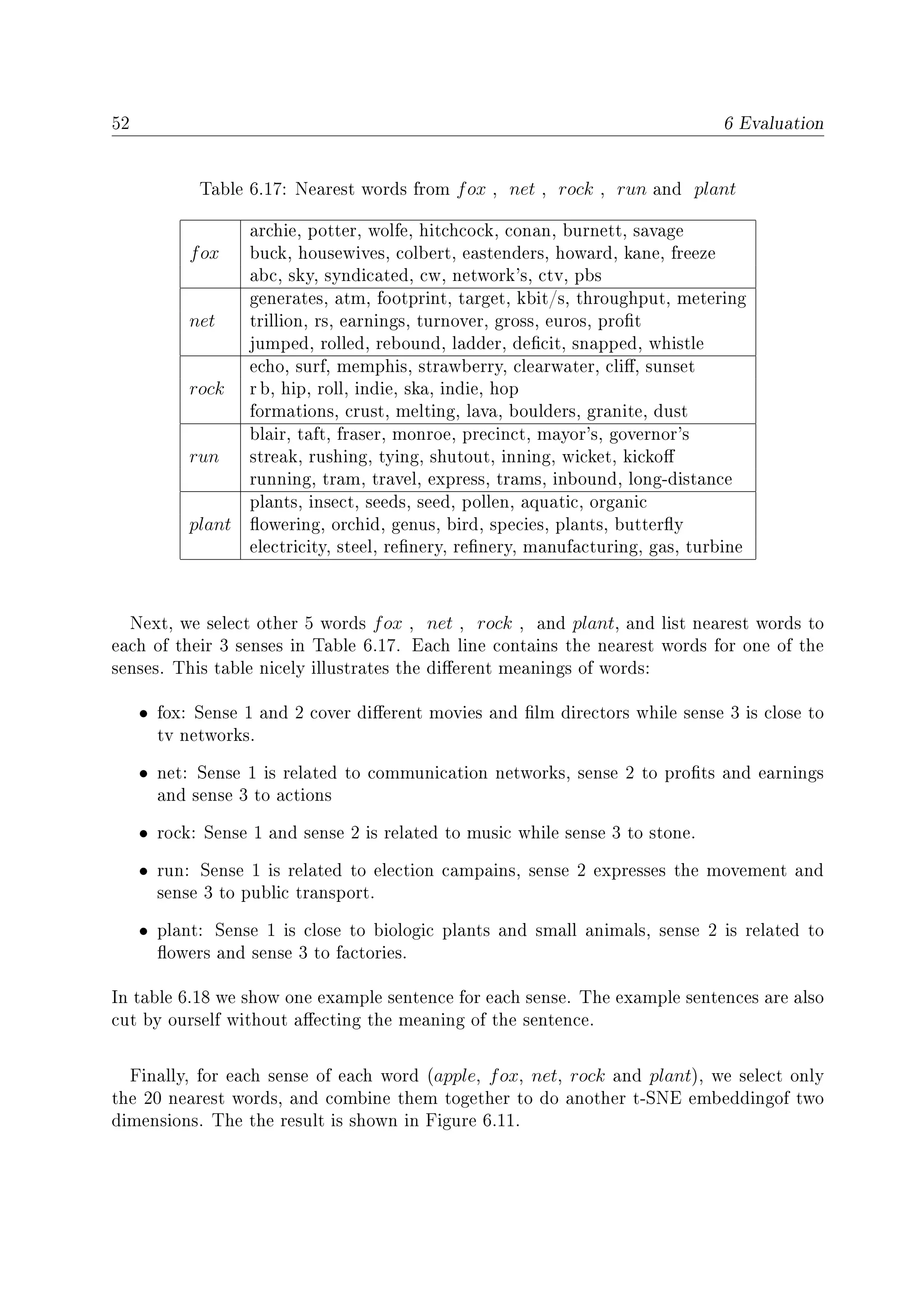
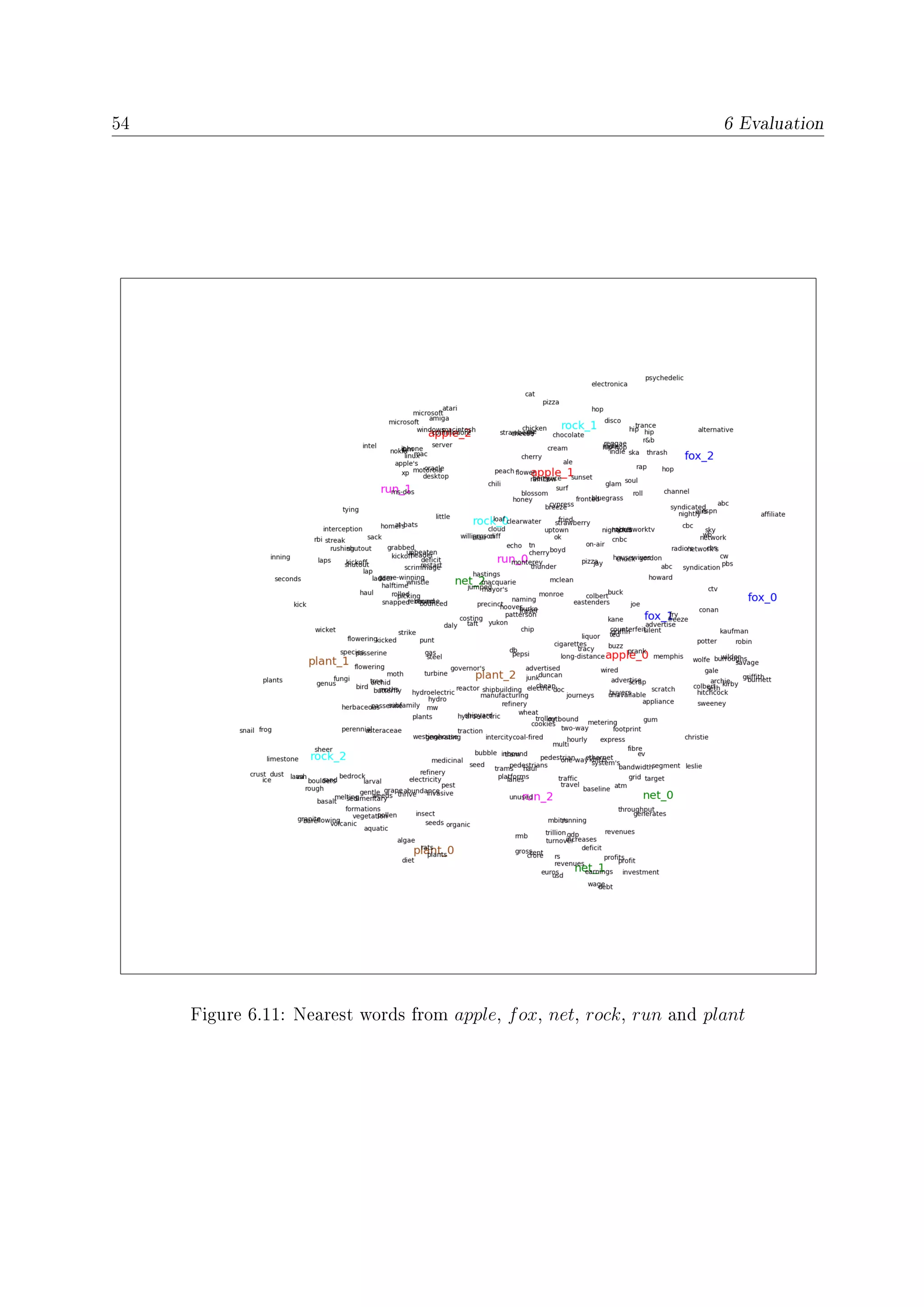
6.2 Case Analysis
In the following, we will select only one experiment's result to do the visualization of senses
and compute nearest word senses. The selection is based on the nal loss and similarity
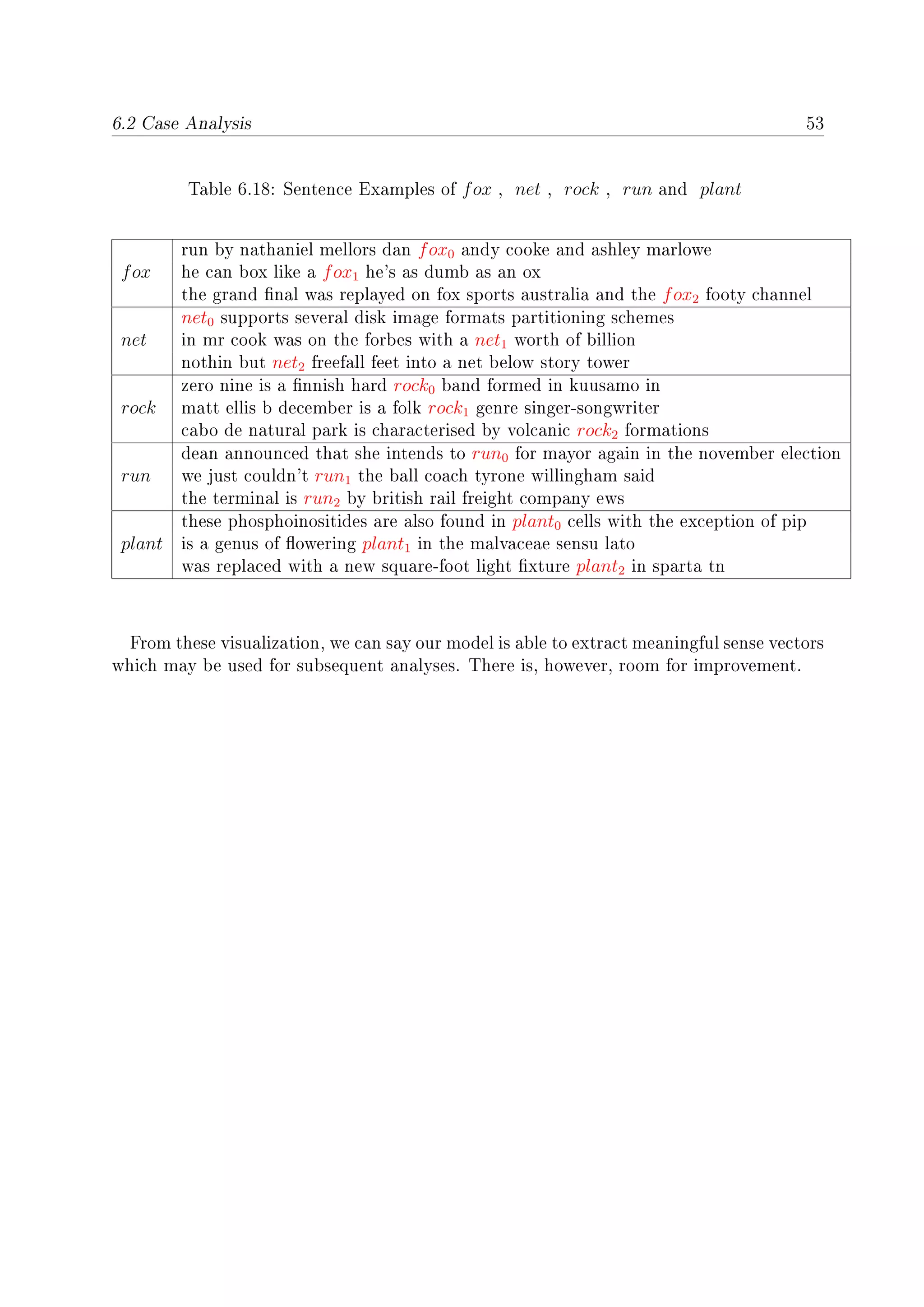
task, specically it is experiment 13 from above.](https://image.slidesharecdn.com/eafda45f-0c51-4ed1-b9f3-f7670fd415ea-160726141620/75/HaiqingWang-MasterThesis-64-2048.jpg)
![50 6 Evaluation
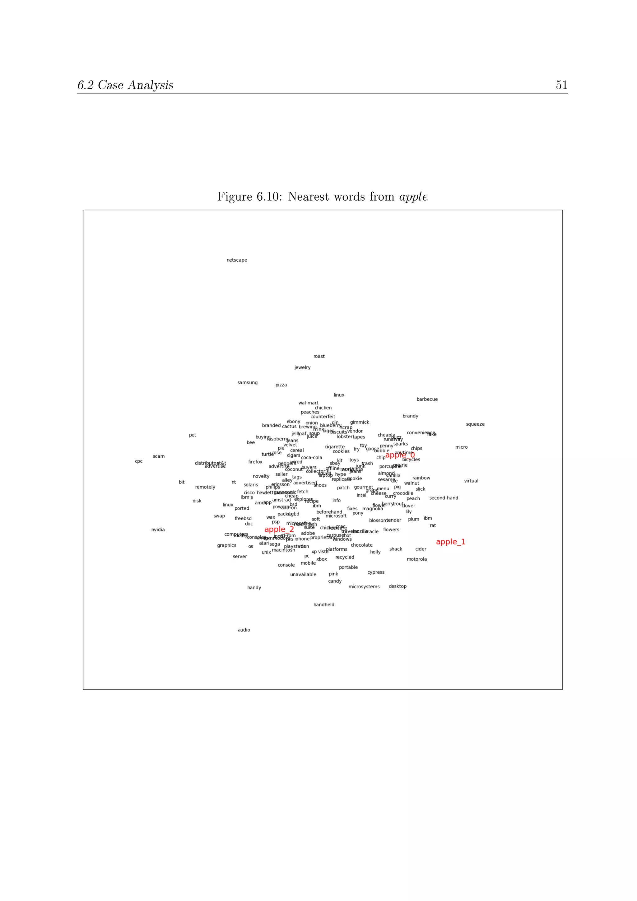
Table 6.15: Nearest Words of apple
apple0: cheap , junk , scrap , advertised , gum , liquor , pizza
apple1: chocolate, chicken, cherry, berry, cream, pizza, strawberry
apple2: macintosh, linux, ibm, amiga, atari, commodore, server
Table 6.16: Sentence Examples of apple
apple0
he can't tell an onion from an apple0 and he's your eye witness
some fruits e.g apple0 pear quince will be ground
apple1
the cultivar is not to be confused with the dutch rubens apple1
the rome beauty apple1 was developed by joel gillette
apple2
a list of all apple2 internal and external drives in chronological order
the game was made available for the apple2 iphone os mobile platform
To visualize semantic neighborhoods we selected 100 nearest words for each sense of apple
and use t-SNE algorithm [Maaten and Hinton, 2008] to project the embedding vectors into
two dimensions. And then we only displayed 70% of words randomly to make visualization
better, which is shown in Figure 6.10.](https://image.slidesharecdn.com/eafda45f-0c51-4ed1-b9f3-f7670fd415ea-160726141620/75/HaiqingWang-MasterThesis-66-2048.jpg)
![Chapter 7
Conclusion
This thesis had the goal to develop an algorithm to estimate multiple sense embeddings per
word and implement this algorithm in the parallel execution framework Spark. We were
able to develop such an algorithm based on the Skip-gram model of Mikolov et al. [2013].
The implementation in the Spark framework in terms of the programming language Scala
and the understanding of the setup parameters and the functionality of Spark were a major
task. Nevertheless the spark framework is very convenient to use. Especially dicult was
the testing of derivatives which was done by nite dierence approximation. Originally
our model assumes that for each word both input embedding and output embedding have
multiple senses. But the experiment results told us, the performance would be better if
the output embeddings have only one sense. We displayed the nearest words of dierent
senses from the same word. The result showed that our model can really derive expres-
sive sense embeddings, which achieved our goal. And the experiments showed that our
implementation is quite ecient, that is also our goal.
However, the evaluation on similarity tasks seems not very satisfying comparing with other
approaches. This may have two possible reasons. Note, that due to time constraints we
were not able to explore many combinations of model hyper-parameters. In addition we had
no time to optimize the conguration of Spark (e.g. memory assignment, number of data
batches collected in RDDs, etc.) to be able to do an exhaustive training on many cluster
nodes. In the future we plan to improve our model. We will try bigger sizes of embedding
vectors. On the other hand, we can also modify preprocessing such as to remove the stop
words, which may also improve our results. And the maximum number of senses in our
model is only three. We will increase the number of senses and try to extend our model so
that it can decide the number of senses for each word similar to (Neelakantan et al. [2015]).
Further more, we think we can do more experiments for the dierent hyper-parameters in
the future to make our results more reliable.
55](https://image.slidesharecdn.com/eafda45f-0c51-4ed1-b9f3-f7670fd415ea-160726141620/75/HaiqingWang-MasterThesis-71-2048.jpg)