This document provides an introduction and table of contents for a book titled "Computational Thinking: A Primer for Programmers and Data Scientists". The book aims to introduce computational thinking concepts to laypeople through hands-on examples and exercises using sample datasets. It is organized into three parts covering foundational computational thinking topics, applications for data science, and more advanced concepts. An interactive digital version will also be released to provide hands-on practice of problem solutions.


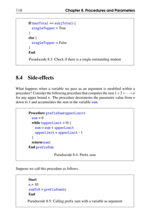
![3.4 Average 49
Start
Initialisation: Arrange cards in "unseen"
pile; keep free space for "seen" pile
Initialise sum to 0 and count to 0
More cards in
"unseen" pile?
Pick one card X from the "unseen" pile
and and move it into the "seen" pile
Add X.F to sum and Increment count
Store sum/count
in average
End
No (False)
Yes (True)
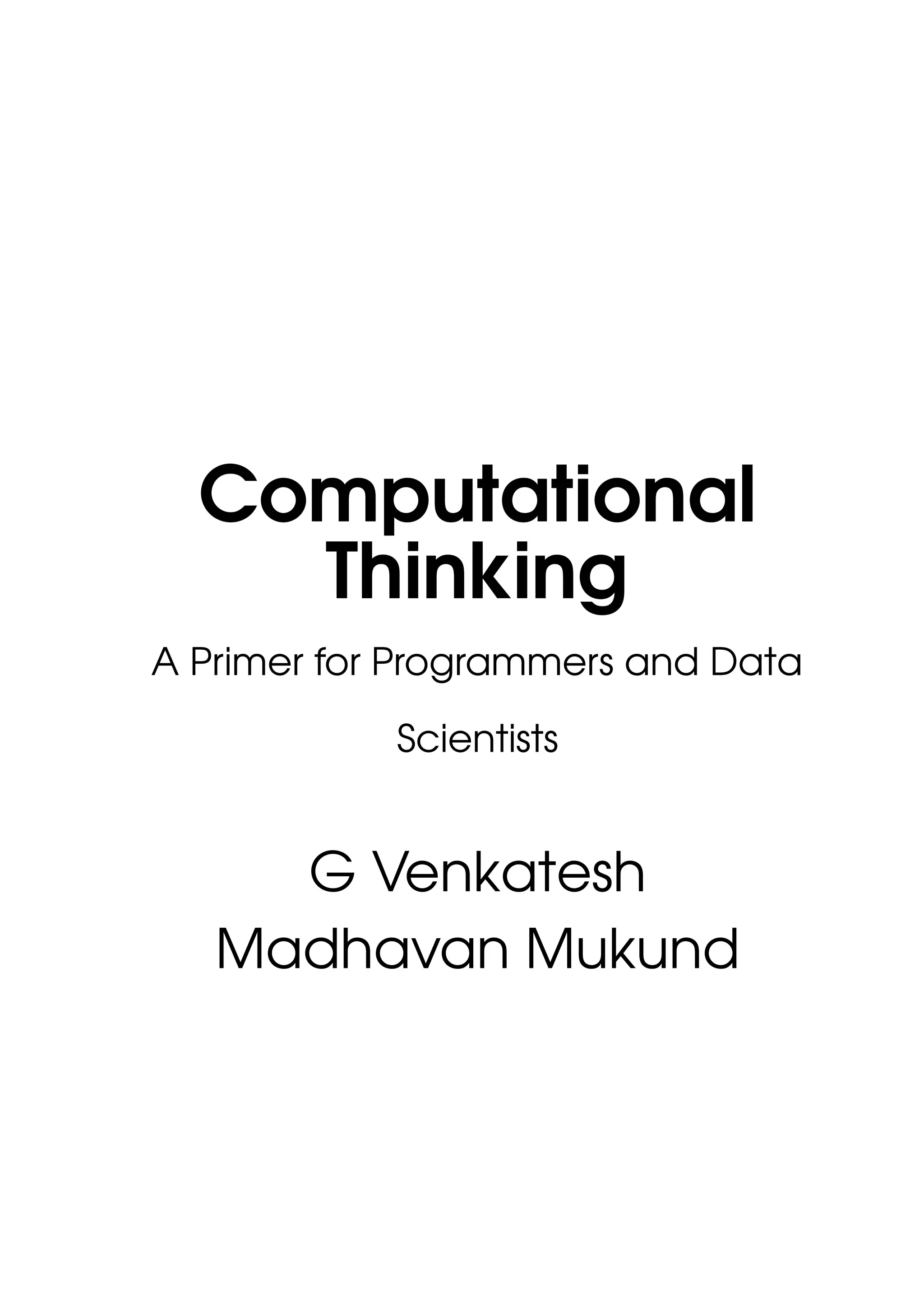
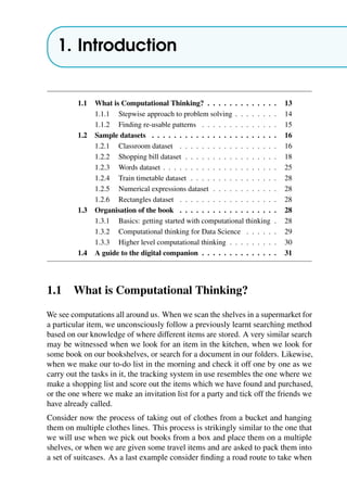
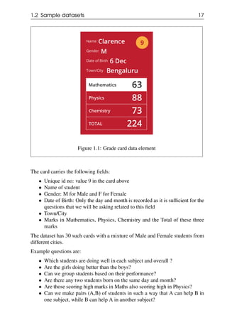
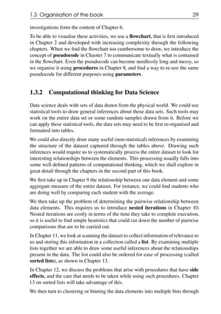
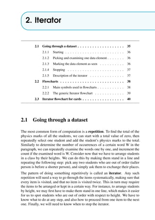
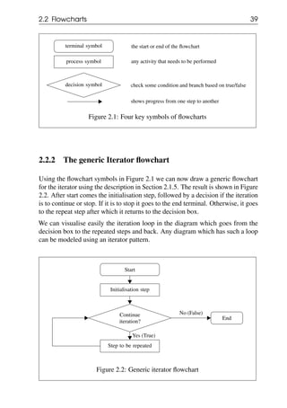
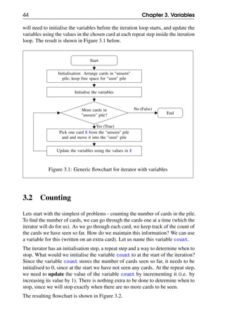
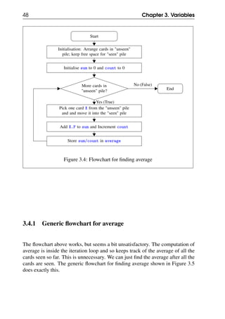
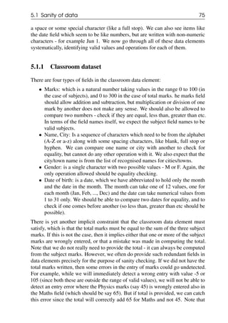
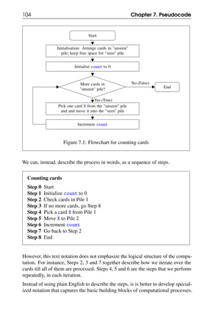
Figure 3.5: Generic flowchart for finding average
We can use this generic flowchart for finding the average physics marks of all
students - just replace X.F in the flowchart above by X.physicsMarks. Similarly
to find the average letter count, we can replace it by X.letterCount.
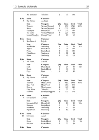
3.4.2 Harder example: Centre of gravity of rectangles
3.4.3 Collecting values in a list
What are the intermediate values that we can store in a variable? Is it only numbers,
or can we also store other kinds of data in the variables? We will discuss this
in more detail in Chapter 5. But for now, let us consider just the example of
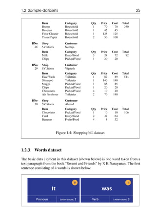
collecting field values into a variable using what is called a list. An example of a
list consisting of marks is [46, 88, 92, 55, 88, 75]. Note that the same element can
occur more than once in the list.
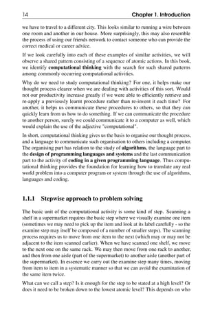
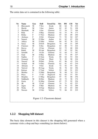
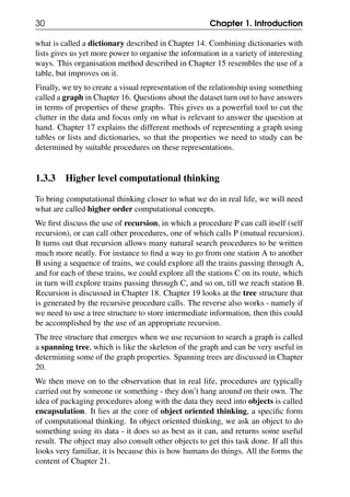
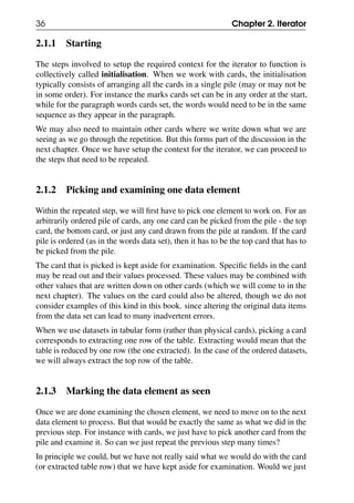
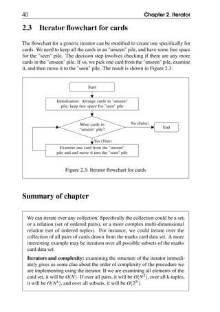
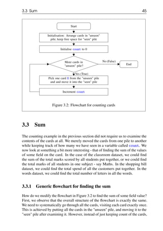
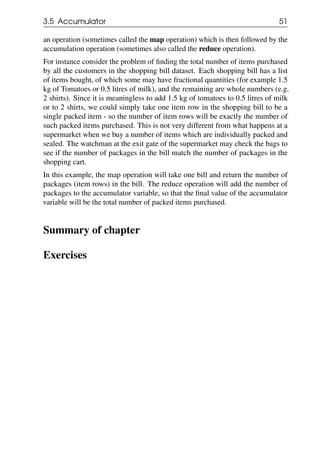
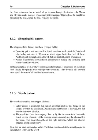
The flowchart shown below in Figure 3.6 collects all the Physics marks from all
the cards in the list variable marksList. It is initialised to [] which represents the
empty list. The operation append M to marksList adds a mark M to the end of
the list - i.e. if marksList is [a1,a2,a3,...,ak] before we append M, then it will
be [a1,a2,a3,...,ak,M] after the append operation.](https://image.slidesharecdn.com/computationalthinkingv0-210911102527/85/Computational-thinking-v0-1_13-oct-2020-49-320.jpg)
![50 Chapter 3. Variables
Start
Initialisation: Arrange cards in "unseen"
pile; keep free space for "seen" pile
Initialise marksList to []
More cards in
"unseen" pile?
Pick one card X from the "unseen" pile
and and move it into the "seen" pile
Append X.physicsMarks to marksList
End
No (False)
Yes (True)
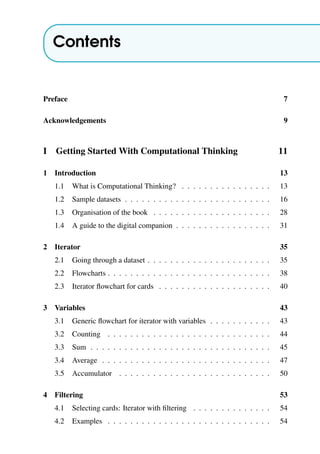
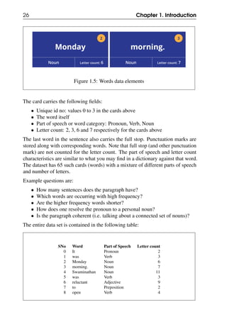
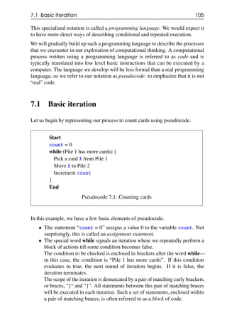
Figure 3.6: Flowchart for collecting all the Physics marks
3.5 Accumulator
Note the similarity between the flowchart for sum and that for collecting the list of
physics marks. In both cases we have a variable that accumulates something - sum
accumulates (adds) the total marks, while marksList accumulates (appends) the
physics marks. The variables were initialised to the value that represents empty -
for sum this was simply 0, while for marksList this was the empty list [].
In general, a pattern in which something is accumulated during the iteration is
simply called an accumulator and the variable used in such a pattern is called an
accumulator variable.
We have seen two simple examples of accumulation - addition and collecting
items into a list. As another example, consider the problem of finding the product
of a set of values. This could be easily done through an accumulator in which
the accumulation operation will be multiplication. But in all of these cases, we
have not really done any processing of the values that were picked up from the
data elements, we just accumulated them into the accumulator variable using the
appropriate operation (addition, appending or multiplication).
The general accumulator will also allow us to first process each element through](https://image.slidesharecdn.com/computationalthinkingv0-210911102527/85/Computational-thinking-v0-1_13-oct-2020-50-320.jpg)

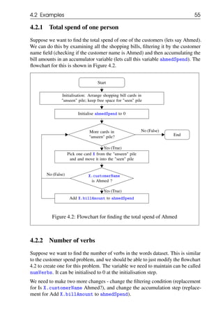
![60 Chapter 4. Filtering
4.2.6 Number of trains on a specific week day
4.2.7 Number of operators in an expression
4.2.8 Harder Example: Number of words in the sentences
Lets consider a slightly harder example now if finding the number of words in all
the sentences of the words dataset.
There are many ways in which this example differs from the ones we have seen
so far. Firstly, when we pick a card from the pile, we will always need to pick
the topmost (i.e. the first) card. This is to ensure that we are examining the cards
in the same sequence as the words in the paragraph. Without this, the collection
words will not reveal anything and we cannot even determine what is a sentence.
Secondly, how do we detect the end of a sentence? We need to look for a word
that ends with a full stop symbol. Any such word will be the last word in a
sentence. Finally, there are many sentences, so the result we are expecting is not a
single number. As we have seen before we can use a list variable to hold multiple
numbers. Lets try and put all this together now.
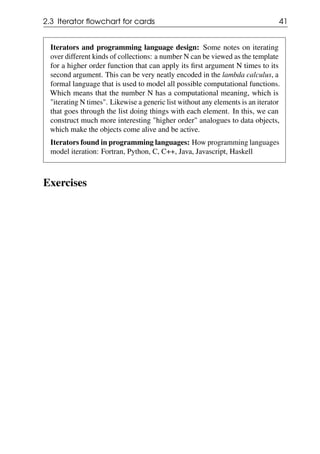
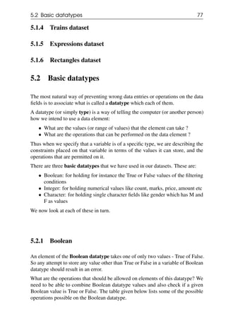
We use a count variable to keep track of the words we have seen so far within
one sentence. How do we do this? We initialise count to 0 at the start of each
sentence, and increment it every time we see a word. At the end of the sentence
(check if the word ends with a full stop), we append the value of count into
a variable swcl which is the sentence word count list. Obviously, we have to
initialise the list swcl to [] during the iterator initialisation step.
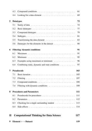
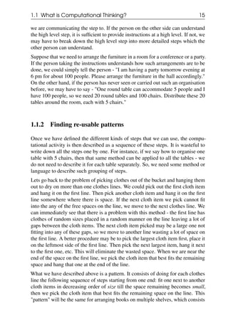
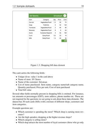
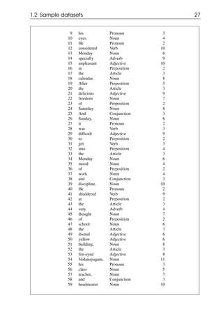
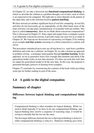
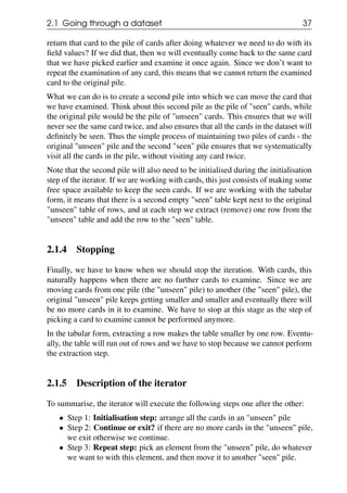
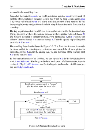
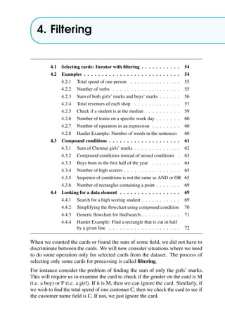
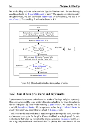
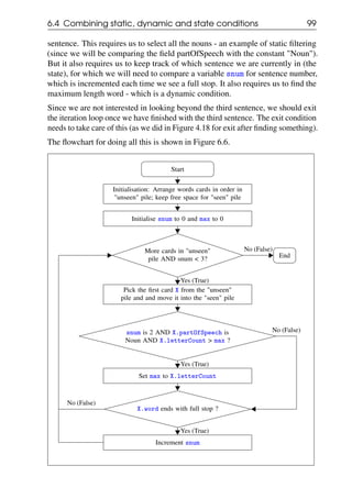
The resulting flowchart is shown in the Figure 4.7 below.](https://image.slidesharecdn.com/computationalthinkingv0-210911102527/85/Computational-thinking-v0-1_13-oct-2020-60-320.jpg)
![4.3 Compound conditions 61
Start
Initialisation: Arrange words cards in order in
"unseen" pile; keep free space for "seen" pile
Initialise count to 0 and swcl to []
More cards in
"unseen" pile?
Pick the first card X from the "unseen"
pile and and move it into the "seen" pile
Increment count
X.word ends
with full stop ?
Append count to swcl and Set count to 0
End
No (False)
Yes (True)
No (False)
Yes (True)
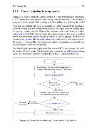
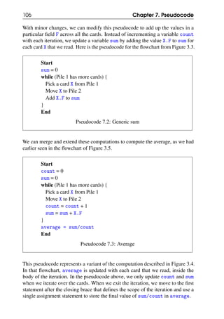
Figure 4.7: Flowchart for finding the word count of all sentences
Note that we do increment of count before the filtering condition check since the
word count in the sentence does not depend on whether we are at the end of the
sentence or not. The filtering condition decides whether the count needs to be
reset to 0 (to start counting words of the next sentence), but before we do the reset,
we first append the existing count value to the list of word counts swcl.
4.3 Compound conditions
In the previous examples, the filtering was done on a single field of the card. In
many situations, the filtering condition may involve multiple fields of the card.
We now look at examples of such compound conditions.](https://image.slidesharecdn.com/computationalthinkingv0-210911102527/85/Computational-thinking-v0-1_13-oct-2020-61-320.jpg)
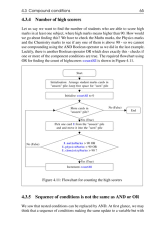
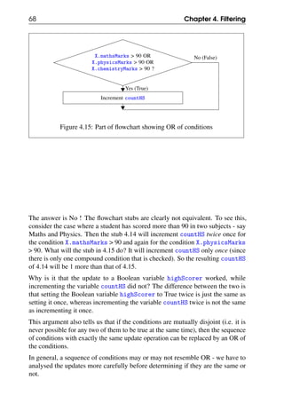
![70 Chapter 4. Filtering
Start
Initialisation: Arrange student marks cards in
"unseen" pile; keep free space for "seen" pile
Initialise highScorers to []
More cards in
"unseen" pile?
Pick one card X from the "unseen" pile
and and move it into the "seen" pile
X.mathsMarks > 90 AND
X.physicsMarks > 90 AND
X.chemistryMarks > 90 ?
Append X.name to highScorers
End
No (False)
Yes (True)
No (False)
Yes (True)
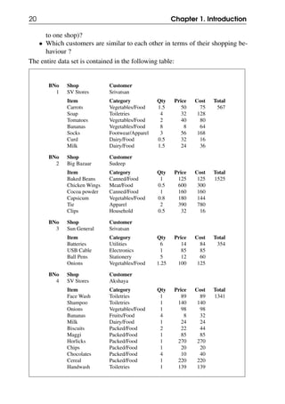
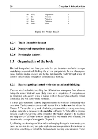
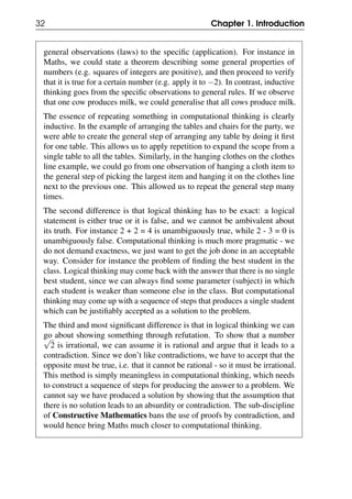
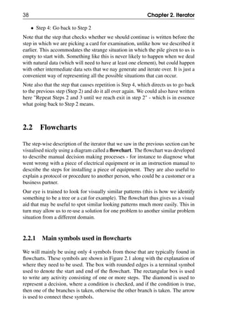
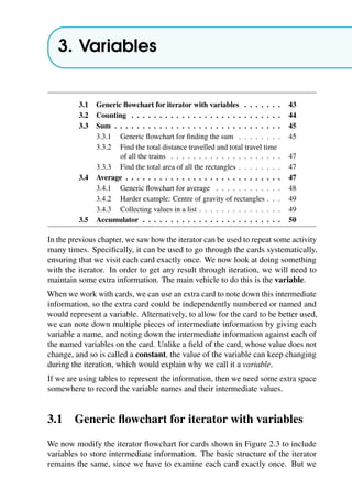
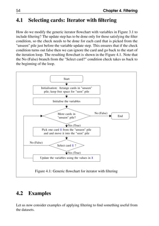
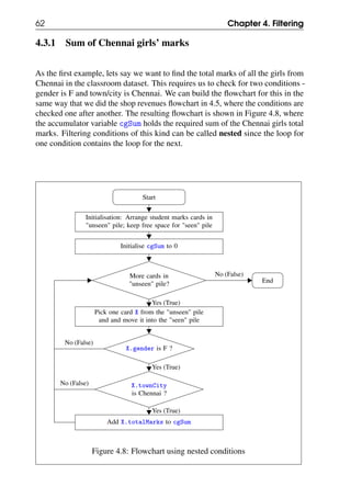
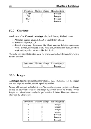
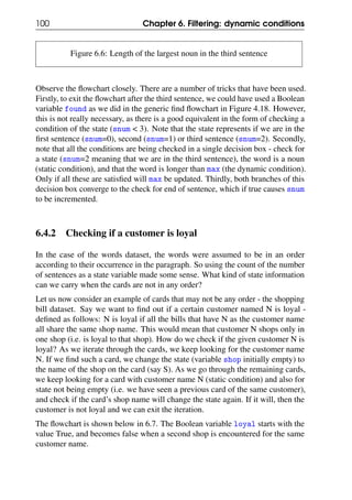
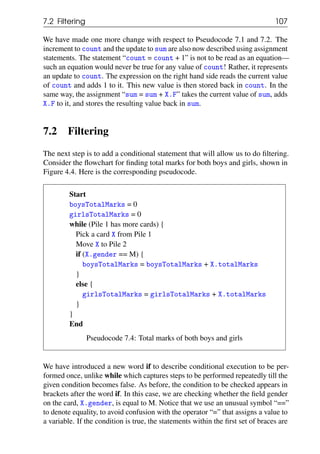
Figure 4.16: Flowchart for searching for a high scorer
Note that rather than go back to the start of the iteration after the append step in
the last activity box, we have exited the iteration loop by going directly to the End
terminal.
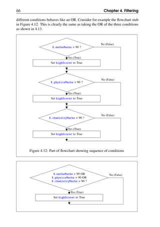
4.4.2 Simplifying the flowchart using compound condition
The flowchart in Figure 4.16 is not very satisfactory as there are two places from
which the iterator can exit - either when the iterator is done with its job (visited all
the cards) or when the item we are searching for is found. In this example, the step
immediately following the completion of the iterator is the End of the procedure,
so it did not turn out that bad. However, when we have to do something with the
values we generate from the iteration (as we saw for example in the example to
find the average in Figure 3.5), we have to know exactly where to go when we
exit from the loop.](https://image.slidesharecdn.com/computationalthinkingv0-210911102527/85/Computational-thinking-v0-1_13-oct-2020-70-320.jpg)
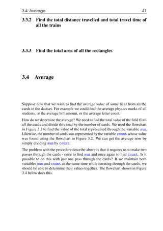
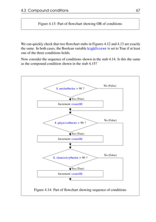
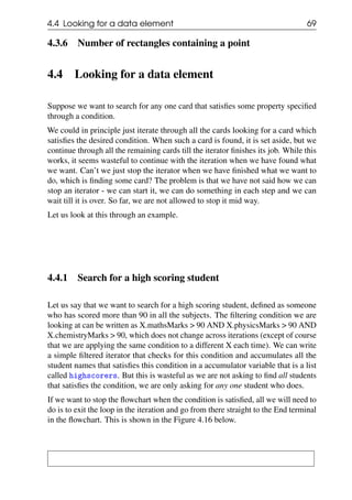
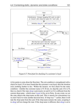
![4.4 Looking for a data element 71
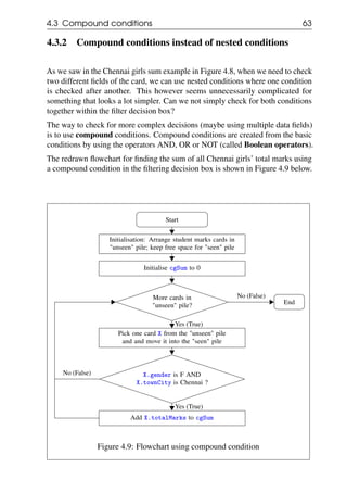
Can we make the exit happen at the same decision box where the iterator checks
for end of iteration? For this we need to extend the exit condition to include
something that checks if the required card has been found. We can do this by
using a new Boolean variable called found, which is initialised to False and turns
True when the required card is found. We then add found to the exit condition
box. This is illustrated in the flowchart in 4.17.
Start
Initialisation: Arrange student marks cards in
"unseen" pile; keep free space for "seen" pile
Initialise highScorers to [] and found to False
More cards in "unseen" pile
AND NOT found ?
Pick one card X from the "unseen" pile
and and move it into the "seen" pile
X.mathsMarks > 90 AND
X.physicsMarks > 90 AND
X.chemistryMarks > 90 ?
Append X.name to highScorers
Set found to True
End
No (False)
Yes (True)
No (False)
Yes (True)
Figure 4.17: High scorer search with single exit point
4.4.3 Generic flowchart for find/search
We can now write the generic flowchart for searching for a card, which can be
adapted for other similar situations. The generic flowchart is shown in Figure
4.18.](https://image.slidesharecdn.com/computationalthinkingv0-210911102527/85/Computational-thinking-v0-1_13-oct-2020-71-320.jpg)
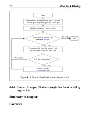
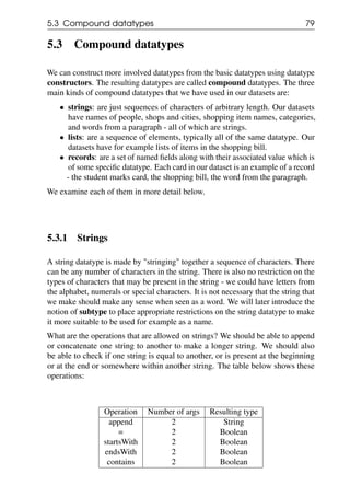
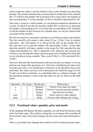
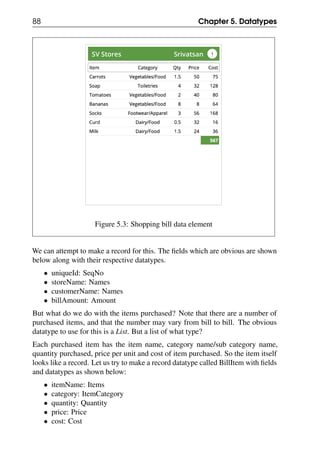
![80 Chapter 5. Datatypes
5.3.2 Lists
Can we collect together several elements, each of which is of some datatype?
There are two mechanisms to do this: lists and records.
In lists, the elements in the collection are not named, and have to be identified
by their position in the list. For instance, in the list L = [a1,a2,a3,...,ak], we can
pick out a3, by going down the list L from the beginning till we get to the third
element.
Typically, all elements in a list are of the same datatype, though this is not strictly
necessary. There is also no restriction on the length of the list.
What are the operations that should be allowed on lists? Firstly, we should be able
to check if the list is the empty list []. We should be able to make a longer list
by putting two lists together (append one list to another), or by inserting a new
element at the beginning of the list. We should also be able to take out the first
element from the list.
Operation No of args Resulting type What it does
append 2 List Appends one list to another
add 2 List Add an element at start of list
= 2 Boolean Check if two lists are equal
isEmpty 1 Boolean Check if the list is empty
head 1 Element’s type First element of the list
tail 1 List List with first element removed
Note that the last two operations head and tail are possible only if the list is not
empty.
5.3.3 Records
Unlike lists, a record is a collection of named fields, with each field having a
name and a value. The value can be of any other datatype. Typically there is no
restriction of any kind in terms of the number of fields or on the datatypes of the
fields.
What operations would we want to perform on the record? The one that we will
need to use for our datasets is that of picking out any field using its name. This
operation is simply denoted by ".", where X.F returns the value of the field F from
the record X. The result type is the same as the type of the field F.](https://image.slidesharecdn.com/computationalthinkingv0-210911102527/85/Computational-thinking-v0-1_13-oct-2020-80-320.jpg)
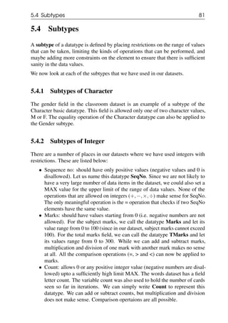
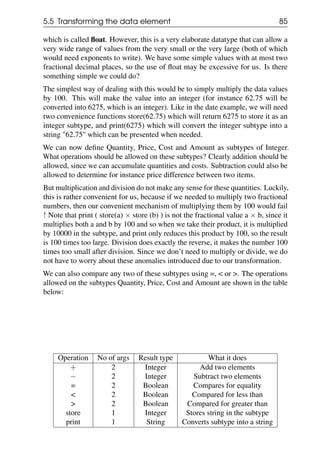
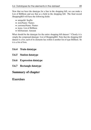

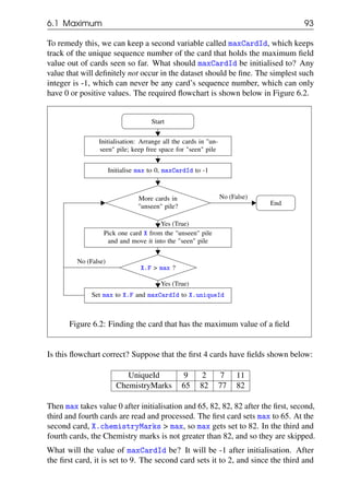
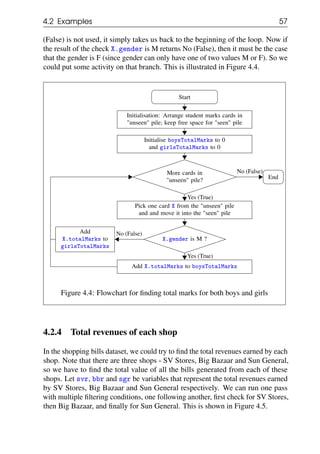
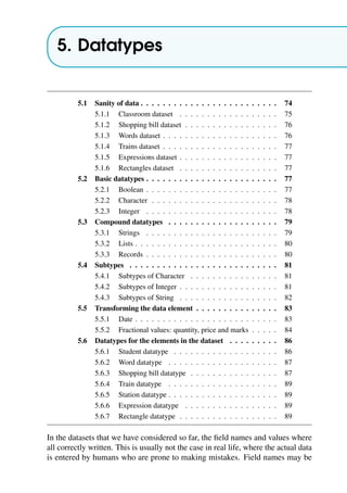
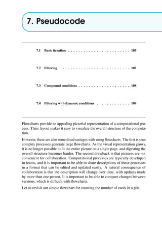
![94 Chapter 6. Filtering: dynamic conditions
fourth card are skipped (filtered out), they don’t change the value of maxCardId.
So, the procedure is correct in the limited sense that it holds one student whose
Chemistry marks is the highest. But this is not so satisfactory since the fourth
card has exactly the same marks as the second card, and it should receive equal
treatment. This would mean that we have to keep both cards, and not just one. We
would need a list variable to hold multiple cards - let us call this list maxCardIds.
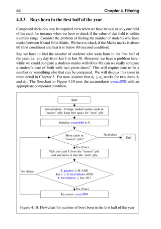
The modified flowchart is shown in Figure 6.3.
Start
Initialisation: Arrange all the cards in "un-
seen" pile; keep free space for "seen" pile
Initialise max to 0, maxCardIds to []
More cards in
"unseen" pile?
Pick one card X from the "unseen" pile
and and move it into the "seen" pile
X.F > max ?
Set max to X.F and maxCardIds to [X.uniqueId]
Append
[X.uniqueId]
to maxCardIds
End
No (False)
Yes (True)
No (False)
Yes (True)
Figure 6.3: Flowchart for finding all the maximum cards
Note that the list variable maxCardIds needs to be initialised to the empty list []
at the start. If we find a card N with a bigger field value than the ones we have
seen so far, the old list needs to be discarded and replaced by [N]. But as we have
seen above, if we see another card M with field value equal to max (82 in the
example above), then we would need to append [M] to the list maxCardIds.
We can apply this flowchart to find all the words with the greatest number of
letters in the Words dataset. For this, replace X.F with X.letterCount.](https://image.slidesharecdn.com/computationalthinkingv0-210911102527/85/Computational-thinking-v0-1_13-oct-2020-94-320.jpg)
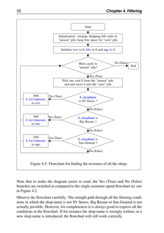
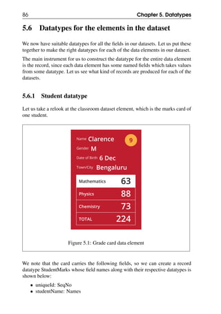
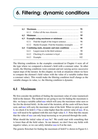
![96 Chapter 6. Filtering: dynamic conditions
Start
Initialisation: Arrange all the cards in "un-
seen" pile; keep free space for "seen" pile
Initialise min to MAX, minCardIds to []
More cards in
"unseen" pile?
Pick one card X from the "unseen" pile
and and move it into the "seen" pile
X.F < min ?
Set min to X.F and minCardIds to [X.uniqueId]
Append
[X.uniqueId]
to minCardIds
End
No (False)
Yes (True)
No (False)
Yes (True)
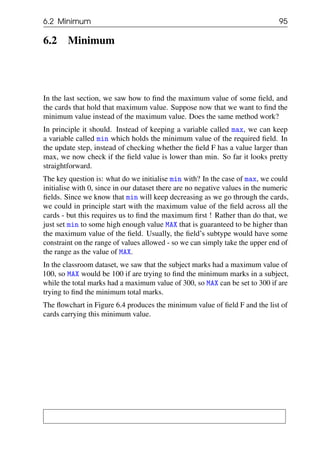
Figure 6.4: Flowchart for finding all the minimum cards
6.3 Examples using maximum or minimum
We now look at examples of situations where the maximum or minimum is
combined with other conditions to make the filtering really dynamic.
6.3.1 Find the length of the longest sentence
Let us now consider a slightly more difficult problem - that of finding the length of
the longest sentence (i.e. the sentence with the largest number of words). For this,
we have to count the words in each sentence, and as we do this we have to keep
track of the maximum value of this count. The flowchart in Figure 4.7 gives us the
word count of all the sentences. Can we modify it to give us just the maximum
count rather than the list of all the sentence word counts? The required flowchart
is shown in Figure 6.5.](https://image.slidesharecdn.com/computationalthinkingv0-210911102527/85/Computational-thinking-v0-1_13-oct-2020-96-320.jpg)
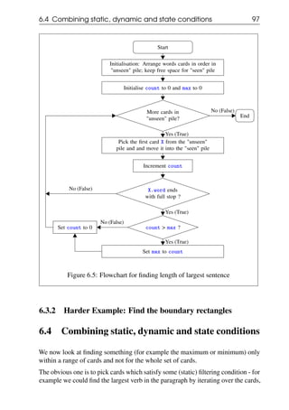


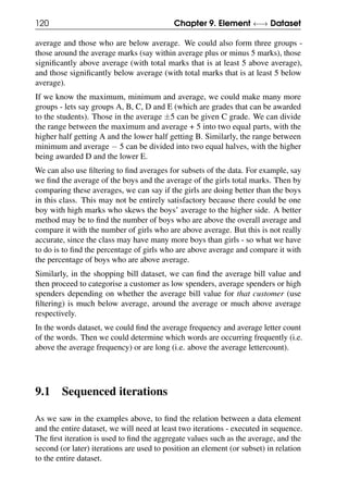
![9.2 Compare with average 123
could determine the average only for a subset of the data elements, and compare
these with the average of the whole, which may reveal something about that
subset.
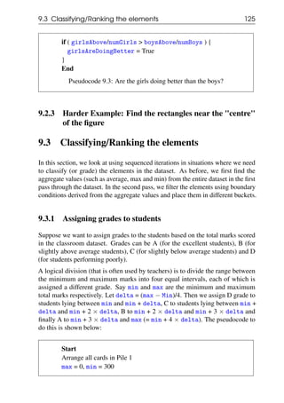
9.2.1 Students performing well
Let us say we want to find out which students are doing well. How do we define
"doing well"? We could start with a simple definition - say doing well is the same
as above average. The pseudocode pattern for sequential iteration can be modified
to do this as shown below:
Start
Arrange all cards in Pile 1
sum = 0, count = 0
while (Pile 1 has more cards) {
Pick a card X from Pile 1
Move X to Pile 2
sum = sum + X.totalMarks
count = count + 1
}
average = sum/count
Arrange all cards in Pile 1
aboveList = []
while (Pile 1 has more cards) {
Pick a card X from Pile 1
Move X to Pile 2
if (X.totalMarks > average) {
Append [X] to aboveList
}
}
End
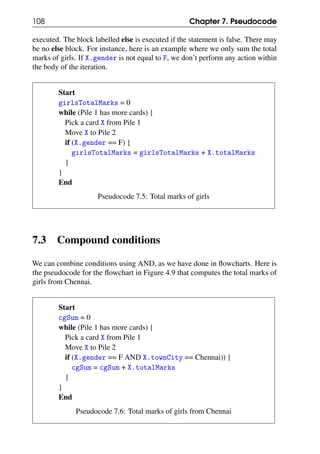
Pseudocode 9.2: Above average students
9.2.2 Are the girls doing better than the boys?
As we discussed at the beginning of the chapter, to find out if the girls are doing
better than the boys, we could find the percentage of girls who are above the](https://image.slidesharecdn.com/computationalthinkingv0-210911102527/85/Computational-thinking-v0-1_13-oct-2020-123-320.jpg)
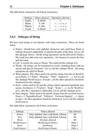
![126 Chapter 9. Element ←→ Dataset
while (Pile 1 has more cards) {
Pick a card X from Pile 1
Move X to Pile 2
if ( X.totalMarks > max ) {
max = X.totalMarks
}
if ( X.totalMarks < min ) {
min = X.totalMarks
}
}
delta = (max - min)/4
Arrange all cards in Pile 1
listA = [], listB = [], listC = [], listD = []
while (Pile 1 has more cards) {
Pick a card X from Pile 1
Move X to Pile 2
if (X.totalMarks < min + delta) {
Append [X] to listD
}
else if (X.totalMarks < min + 2 × delta) {
Append [X] to listC
}
else if (X.totalMarks < min + 3 × delta) {
Append [X] to listB
}
else {
Append [X] to listA
}
}
End
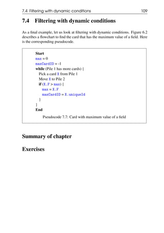
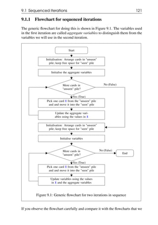
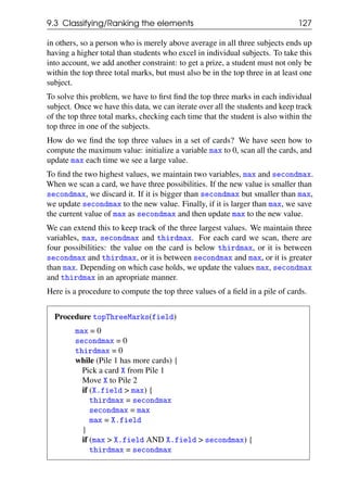
Pseudocode 9.4: Assigning grades to students
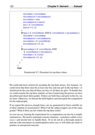
9.3.2 Awarding 3 prizes to the top students
Suppose we want to award prizes to the three best students in the class. The
most obvious criterion is to choose the students with the three highest total marks.
However, we may have a situation where students excel in one subject but not](https://image.slidesharecdn.com/computationalthinkingv0-210911102527/85/Computational-thinking-v0-1_13-oct-2020-126-320.jpg)


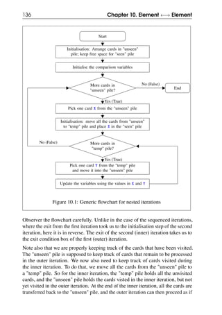
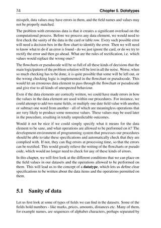
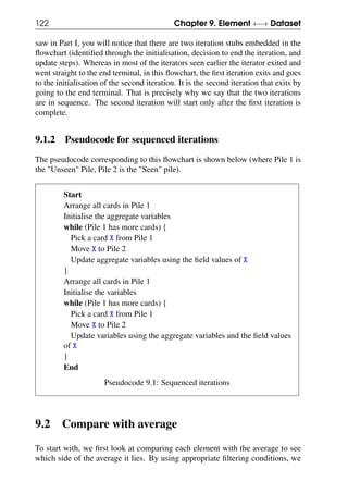
![10.1 Nested iterations 139
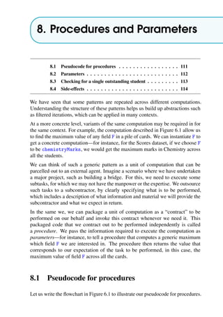
10.1.4 Alternate pseudocode for nested iterations
The pseudocode for this alternate nested iteration is shown below, where Pile 1 is
the "unseen" pile, Pile 2 is the "seen" pile and Pile 3 is the "temp" pile.
Start
Arrange all cards in Pile 1, Initialise the variables
while (Pile 1 has more cards) {
Pick a card X from Pile 1
Move all cards from Pile 2 to Pile 3
Move X to Pile 2
while (Pile 3 has more cards) {
Pick a card Y from Pile 3
Move Y to Pile 2
Update variables using the field values of X and Y
}
}
End
Pseudocode 10.2: Another way to do nested iterations
10.1.5 List of all pairs of elements
As the first example, let us just return all the pairs of elements as a list pairsList.
The pseudocode to do this 9using the alternate method above) is shown below.
Start
Arrange all cards in Pile 1, Initialise pairsList to []
while (Pile 1 has more cards) {
Pick a card X from Pile 1
Move all cards from Pile 2 to Pile 3
Move X to Pile 2
while (Pile 3 has more cards) {
Pick a card Y from Pile 3
Move Y to Pile 2
Append [ (X,Y) ] to pairsList
}
}](https://image.slidesharecdn.com/computationalthinkingv0-210911102527/85/Computational-thinking-v0-1_13-oct-2020-139-320.jpg)
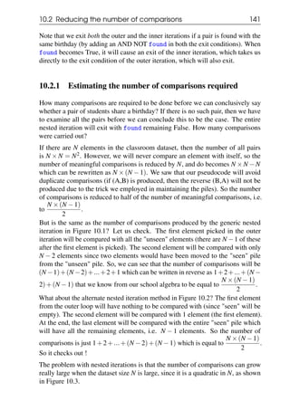
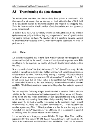
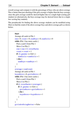
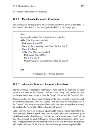
![10.2 Reducing the number of comparisons 143
10.2.2 Using binning to reduce the number of comparisons
As we saw above, the number of comparison pairs in nested iterations grows
quadratically with the number of elements. This becomes a major issue with large
datasets. Can we somehow reduce the number of comparisons to make it more
manageable?
In the example above where we are trying to find two students with the same
birthday, the problem has a deeper structure that we can exploit. Note that two
students will share the same birthday only if firstly they share the same month of
birth. Which means that there is simply no sense in comparing two students if
they are born in different months. This should result in a substantial reduction in
comparisons.
In order to take advantage of this, we have to first separate the students into bins,
one for each month. Let us name the bins Bin[1], Bin[2], ..., Bin[12]. So for
example, Bin[3] will be the list of all students who are born in March. We should
first process all the cards in the classroom dataset and put each of them in the
correct bin. Once this is done, we can go through the bins one by one and compare
each pair of cards within the bin.
The pseudocode to do this is shown below. It uses a procedure processBin(bin)
to do all the comparisons within each bin, whose body will be exactly the same
as the Same birthday pseudocode that we saw earlier, except that instead of
processing the entire classroom dataset, it will process only the cards in Bin[i]
and return the value of found. The procedure month(X) returns the month part of
X.dateOfBirth as a numeral between 1 and 12.
Start
Arrange all cards from the classroom dataset in Pile 1
Initialise Bin[i] to [] for all i from 1 to 12
while (Pile 1 has more cards) {
Pick a card X from Pile 1
Move X to Pile 2
Append [X] to Bin[month(X)]
}
found = False, i = 1
while (i < 13 AND NOT found) {
found = processBin(Bin[i])
i = i + 1
}](https://image.slidesharecdn.com/computationalthinkingv0-210911102527/85/Computational-thinking-v0-1_13-oct-2020-143-320.jpg)
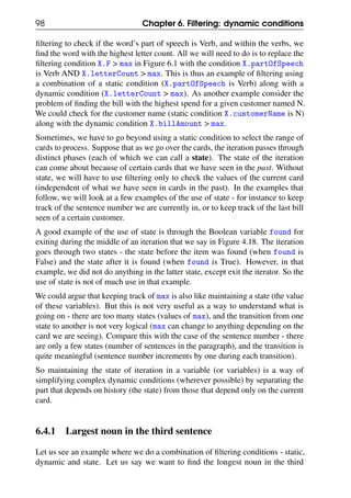
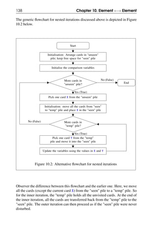
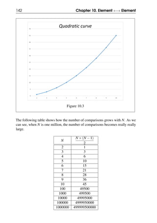
![144 Chapter 10. Element ←→ Element
End
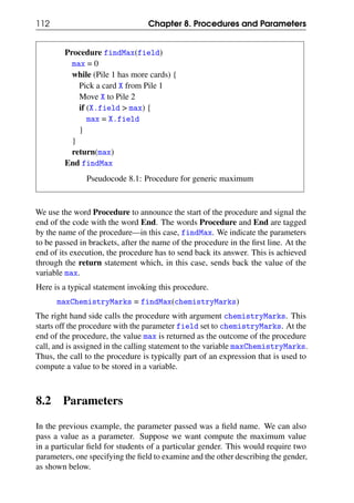
Pseudocode 10.5: Same birthday using binning
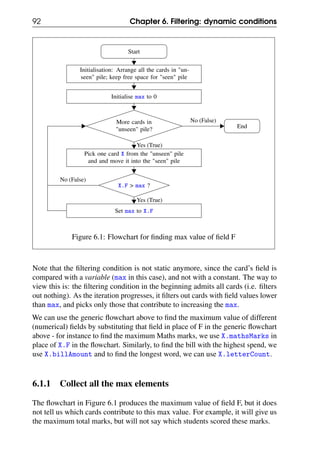
10.2.3 Improvement achieved due to binning
can we make an estimate of the reduction in comparisons achieved through
binning? Let us look at the boundary conditions first. If all the students in the
classroom dataset happen to have the same month of birth, then there is simply no
reduction in the number of comparisons ! So, in the worst case, binning achieves
nothing.
At the other extreme, consider the situation where the students are equally dis-
tributed into the 12 bins Bin[1],...,Bin[12] (of course this also means that the total
number of students N is a multiple of 12. Clearly, this will yield the least number
of comparisons. The size of each bin will be N/12 and the number of compar-
isons within each bin will be
N/12×(N/12−1)
2
=
N ×(N −12)
288
. Then the total
number of comparisons is just 12 times this number, i.e. it is
N ×(N −12)
24
.
Say N = 36, then the number of comparisons without binning would be
N ×(N −1)
2
=
36×35
2
= 630. With binning, it would be
N ×(N −12)
24
=
36×24
24
= 36. So,
we have reduced 630 comparisons to just 36 comparisons ! The reduction factor
R tells us by how many times the number of comparisons has reduced. In this
example, the number of comparison is reduced by R = 630/36 = 17.5 times.
In the general case, if the number of bins is K, and the N elements are equally
divided into the bins, then we can easily calculate the reduction factor in the same
manner as above to be R =
N −1
N/K −1
.
In most practical situations, we are not likely to see such an extreme case where
all students have the same month of birth. Nor is it likely that the students will
be equally distributed into the different bins. So, the reduction in number of
comparisons will be somewhere between 0 and R times.](https://image.slidesharecdn.com/computationalthinkingv0-210911102527/85/Computational-thinking-v0-1_13-oct-2020-144-320.jpg)
![10.3 Examples of nested iterations 145
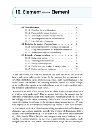
10.3 Examples of nested iterations
We now look at a few more examples of finding pairs of elements using nested
iterations. In each case, we will try to reduce the number of comparisons by using
binning wherever possible. If binning does not work, we will try to use some
other structural information in the problem (such as state) to reduce the number
of comparisons.
10.3.1 Study group pairing
In any class, students typically pair up (or form small groups), so that within each
pair, one student can help the other in at least one subject. For a study pair (A,B)
to be meaningful, A has to be able to help B in some subject. This will clearly
benefit B (at least for that subject). For this to be of benefit to A, it should also be
the case that B can help A in some other subject. When can we say that A can
help B in a subject? We can define this as A’s marks in some subject is at least
10 marks more than that of B in that subject. So (A,B) would form a meaningful
study pair if there are subjects S1 and S2 such that A’s marks exceeds B’s marks in
S1 by at least 10, and B’s marks exceeds A’s marks in S2 by at least 10.
The pseudocode for finding the study pairs taking into account only two subjects
Maths and Physics is shown below. The result is a list studyPairs of student
pairs who can help each other.
Start
Arrange all cards from the classroom dataset in Pile 1
studyPairs = []
while (Pile 1 has more cards) {
Pick a card X from Pile 1
Move all remaining cards from Pile 1 to Pile 3
Move X to Pile 2
while (Pile 3 has more cards) {
Pick a card Y from Pile 3
Move Y to Pile 1
if (X.mathsMarks - Y.mathsMarks > 9 AND
Y.physicsMarks - X.physicsMarks > 9) {
Append [(X, Y)] to studyPairs
}
if (Y.mathsMarks - X.mathsMarks > 9 AND](https://image.slidesharecdn.com/computationalthinkingv0-210911102527/85/Computational-thinking-v0-1_13-oct-2020-145-320.jpg)
![146 Chapter 10. Element ←→ Element
X.physicsMarks - Y.physicsMarks > 9) {
Append [(X, Y)] to studyPairs
}
}
}
End
Pseudocode 10.6: Study group pairing
The number of comparisons in this pseudocode will be large because we are
comparing every student with every other student. Can we reduce the number of
comparisons using some form of binning?
There is no obvious field that we can use (like the month of birth in the case of
the same birthday problem). But, we can make a simplification which could help
us. Observe that if a pair (A,B) is produced by the above pseudocode, then A
should be better than B in either Maths (or Physics), and B should be better in A
in Physics (or Maths). This would mean that it is quite likely that the sum of the
Maths and Physics marks will be roughly the same ! Of course, this need not be
always true, but if it works in most of the cases, that is good enough for us. Such
simplifying assumptions that works in most cases is called a heuristic.
Now that we have this simplifying heuristic, we can bin the students into groups
based on their sum of the Maths and Physics marks. This sum can be any number
between 0 and 200, but since most of the students have marks above 50, we
are more likely to find the range to be between 100 and 200. So let us bin the
students according to whether the sum of their Maths and Physics marks is in the
ranges 0-125, 125-150, 150-175 or 175-200, which gives us 4 bins to work with.
Let us call these bins binD, binC, binB and binA (as if we are awarding grades
to the students based on the sum of their Maths and Physics marks). Then the
simplifying heuristic tells us that we should look for pairs only within a bin and
not across bins.
Let us first convert the pseudocode in 10.6 into a procedure that works within one
bin.
Procedure processBin(bin)
Arrange all cards from bin in Pile 1
binPairs = []
while (Pile 1 has more cards) {
Pick a card X from Pile 1](https://image.slidesharecdn.com/computationalthinkingv0-210911102527/85/Computational-thinking-v0-1_13-oct-2020-146-320.jpg)
![10.3 Examples of nested iterations 147
Move all remaining cards from Pile 1 to Pile 3
Move X to Pile 2
while (Pile 3 has more cards) {
Pick a card Y from Pile 3
Move Y to Pile 1
if (X.mathsMarks - Y.mathsMarks > 9 AND
Y.physicsMarks - X.physicsMarks > 9) {
Append [(X, Y)] to binPairs
}
if (Y.mathsMarks - X.mathsMarks > 9 AND
X.physicsMarks - Y.physicsMarks > 9) {
Append [(X, Y)] to binPairs
}
}
}
return (binPairs)
End processBin
Pseudocode 10.7: Study group pairing procedure
The pseudocode for finding study pairs using binning is now shown below.
Start
Arrange all cards from the classroom dataset in Pile 1
Initialise binA to [], binB to [], binC to [], binD to []
while (Pile 1 has more cards) {
Pick a card X from Pile 1
Move X to Pile
if (X.mathsMarks + X.physicsMarks < 125) {
Append [X] to binD
}
else if (X.mathsMarks + X.physicsMarks < 150) {
Append [X] to binC
}
else if (X.mathsMarks + X.physicsMarks < 175) {
Append [X] to binB
}](https://image.slidesharecdn.com/computationalthinkingv0-210911102527/85/Computational-thinking-v0-1_13-oct-2020-147-320.jpg)
![148 Chapter 10. Element ←→ Element
else {
Append [X] to binA
}
}
studyPairs = []
Append processBin (binA) to studyPairs
Append processBin (binB) to studyPairs
Append processBin (binC) to studyPairs
Append processBin (binD) to studyPairs
End
Pseudocode 10.8: Study group pairing using binning
Note that through the use of a simplifying heuristic (that we are more likely to find
pairs within the bins rather than across the bins), we can reduce the comparisons
substantially.
10.3.2 Matching pronouns to nouns
Let us now turn our attention to the words dataset, which are words drawn from a
paragraph. Typically, a paragraph is broken down into sentences, each of which
could be a simple sentence (i.e. has a single clause) or a compound sentence
(made of multiple clauses connected by a comma, semicolon or a conjunction).
The sentence itself will have a verb, some nouns and perhaps some adjectives
or adverbs to qualify the nouns and verbs. In most sentences, the noun will be
replaced by a short form of the noun, called a pronoun. For instance the first
sentence may use the name of a person as the noun (such as Swaminathan), while
subsequent references to this person may be depicted using an appropriate personal
pronoun (he, his, him etc).
Now, the question we are asking here is this: given a particular personal pronoun
(such as the word "he"), can we determine who this "he" refers to in the paragraph?
Clearly, "he" has to refer to a male person - so we can look at an appropriate
word that represents a name (and hopefully a male name). If we look back from
the pronoun word "he" one word at a time, we should be able to find the closest
personal noun that occurs before this pronoun. Maybe that is the person which is
referred to by "he"? This is a good first approximation to the solution. So let us
see how to write it in pseudocode form.
Note that unlike in the other datasets, in the words dataset, the order of the words](https://image.slidesharecdn.com/computationalthinkingv0-210911102527/85/Computational-thinking-v0-1_13-oct-2020-148-320.jpg)
![10.3 Examples of nested iterations 149
matters (since the meaning of a sentence changes entirely or becomes meaningless
if the words are jumbled). Note also that for a given pronoun, we have to search
all the cards before that pronoun to look for a personal noun, and that we will
search in a specific order - we start from the word just before the pronoun and
start moving back through the words one by one till we find the desired noun.
The pseudocode given below attempts to do find all the possible matches for
each pronoun in a list possibleMatches. It uses the Boolean procedures
isProperName that checks if a noun is a proper name, and personalPronoun
that checks if the pronoun is a personal pronoun (code for both not written here
!). Recall that the "seen" cards will be the words before the current word, while
the "unseen" words will be the ones after the current word. So, the alternate
pseudocode in 10.2 is the one we need to use.
Start
Arrange all words cards in Pile 1 in order
possibleMatches = []
while (Pile 1 has more cards) {
Pick a card X from Pile 1
if (X.partOfSpeech == Pronoun AND
personalPronoun(X.word)) {
Move all cards from Pile 2 to Pile 3 (retaining the order)
while (Pile 3 has more cards) {
Pick the top card Y from Pile 3
Move Y to the bottom of Pile 2
if (Y.partOfSpeech == Noun AND
isProperName(Y.word)) {
Append [(X,Y)] to possibleMatches
}
}
}
Move X to the top of Pile 2
}
End
Pseudocode 10.9: Possible matches for each pronoun
There are a number of interesting things going on in this pseudocode. Firstly
note that we are not carrying out the inner iteration for all the words, we start an
inner iteration only when the current word is a personal pronoun. So, this already
reduces the number of comparisons to be done.](https://image.slidesharecdn.com/computationalthinkingv0-210911102527/85/Computational-thinking-v0-1_13-oct-2020-149-320.jpg)


![Table of contents [data structure and algorithmic thinking with python]](https://cdn.slidesharecdn.com/ss_thumbnails/tableofcontentsdatastructureandalgorithmicthinkingwithpython-150401104714-conversion-gate01-thumbnail.jpg?width=640&height=640&fit=bounds)
![Sample chapters [data structure and algorithmic thinking with python]](https://cdn.slidesharecdn.com/ss_thumbnails/samplechaptersdatastructureandalgorithmicthinkingwithpython-150401104825-conversion-gate01-thumbnail.jpg?width=640&height=640&fit=bounds)


