Berard - Thesis

DIPOLE SOURCE LOCALIZATION USING
ARTIFICIAL NEURAL NETWORKS FOR A
HIGH DEFINITION REALISTIC HEAD MODEL
BY
STEVEN BERARD
A dissertation submitted to the Graduate School
in partial fulﬁllment of the requirements
for the degree
Master of Science
Major Subject: Electrical Engineering
New Mexico State University
Las Cruces New Mexico
December 2013

“Dipole Source Localization Using Artificial Neural Networks for a High Definition
Realistic Head Model,” a thesis prepared by Steven Berard in partial fulfillment
of the requirements for the degree, Master of Science, has been approved and
accepted by the following:
Linda Lacey
Dean of the Graduate School
Dr. Kwong Ng
Chair of the Examining Committee
Date
Committee in charge:
Dr. Kwong Ng, PhD, Chair
Dr. Dr. Nadipuram Prasad, PhD
ii

ACKNOWLEDGMENTS
I would like to thank my advisor, Dr. Kwong Ng, for his encouragement,
advice, and support for the last two years, Dr. Prasad for making me believe
that anything is possible, my parents for always believing in me and helping me
succeed even when I would get in my own way, Dr. Ranade, Dr. De Leon, and the
NMSU College of Engineering for the opportunity to work as a TA while I ﬁnished
this, all my professors for helping prepare for this moment, and my wonderful EE
161 students for always testing me and giving me something to brag about. I also
want to send out a special thank you to Dr. Gert Van Hoey who helped me ﬁnd
my way when I was most lost.
iii

VITA
January 5, 1985 Born in Lancaster, California
January 2008 - December 2009 B.A. in Finance, New Mexico State
University, Las Cruces, NM
August 2012 - December 2013 Graduate Student, New Mexico State
January 2012 - May 2013 Teaching Assistant, New Mexico State
PROFESSIONAL AND HONORARY SOCIETIES
IEEE Student Member
Eta Kappa Nu
PUBLICATIONS
None
iv

ABSTRACT
DIPOLE SOURCE LOCALIZATION USING
ARTIFICIAL NEURAL NETWORKS FOR A
HIGH DEFINITION REALISTIC HEAD MODEL
BY
STEVEN BERARD
Master of Science
New Mexico State University
Las Cruces, New Mexico, 2013
Dr. Kwong Ng, PhD, Chair
It is desired to determine the source of electrical activity in the human brain
with accuracy in real time. Artificial neural networks have been shown do this
in brain-like models, however there are only a limited number of studies on this
subject, and the models used have been of low resolution or simplified geometries.
This paper presents the findings from testing several different neural network
configurations’ ability to source localize within a high fidelity realistic head model
with a resolution of 1 mm × 1 mm × 1 mm with and without noise.
v

CONTENTS
LIST OF TABLES . . . . . . . . . . . . . . . . . . . . . . . . . . . . . x
LIST OF FIGURES . . . . . . . . . . . . . . . . . . . . . . . . . . . . xiv
1 INTRODUCTION . . . . . . . . . . . . . . . . . . . . . . . . . . 1
2 THEORY . . . . . . . . . . . . . . . . . . . . . . . . . . . . . . . 3
2.1 FNS: Finite Difference Neuroelectromagnetic Modeling Software . 3
2.2 Artificial Neural Networks . . . . . . . . . . . . . . . . . . . . . . 4
2.2.1 Backpropagation . . . . . . . . . . . . . . . . . . . . . . . 7
2.2.2 Levenberg-Marquardt Backpropagation . . . . . . . . . . . 8
3 APPROACH . . . . . . . . . . . . . . . . . . . . . . . . . . . . . 12
3.1 2D Headmodel . . . . . . . . . . . . . . . . . . . . . . . . . . . . 12
3.2 Realistic Head Model - Homogeneous Brain Region . . . . . . . . 15
3.3 Realistic Head Model - Complex . . . . . . . . . . . . . . . . . . . 17
4 RESULTS . . . . . . . . . . . . . . . . . . . . . . . . . . . . . . . 20
4.1 2D Head Model . . . . . . . . . . . . . . . . . . . . . . . . . . . . 20
4.2 Realistic Head Model - Homogeneous Brain Region . . . . . . . . 24
4.3 Realistic Head Model - Complex . . . . . . . . . . . . . . . . . . . 29
4.3.1 32 Sensor Configuration - Grid Pattern Training . . . . . . 29
4.3.2 32 Sensor Configuration - Random Pattern Training . . . . 34
vi

4.3.3 64 Sensor Configuration - Grid Pattern Training . . . . . . 41
4.3.4 64 Sensor Configuration - Random Pattern Training . . . . 46
4.3.5 128 Sensor Configuration - Grid Pattern Training . . . . . 53
4.3.6 128 Sensor Configuration - Random Pattern Training . . . 57
5 DISCUSSION . . . . . . . . . . . . . . . . . . . . . . . . . . . . . 64
6 CONCLUSION . . . . . . . . . . . . . . . . . . . . . . . . . . . . 68
REFERENCES . . . . . . . . . . . . . . . . . . . . . . . . . . . . . . . 70
vii

LIST OF TABLES
1 Conductivities for Realistic Head Model with Homogeneous Brain
Region . . . . . . . . . . . . . . . . . . . . . . . . . . . . . . . . . 18
2 Results for 2D Head Model Network 32-30-30-4 . . . . . . . . . . 21
3 Results for Realistic Head Model with Homogeneous Brain Region
(No Noise) . . . . . . . . . . . . . . . . . . . . . . . . . . . . . . . 25
(30 dB SNR) . . . . . . . . . . . . . . . . . . . . . . . . . . . . . 25
(20 dB SNR) . . . . . . . . . . . . . . . . . . . . . . . . . . . . . 27
(10 dB SNR) . . . . . . . . . . . . . . . . . . . . . . . . . . . . . 27
7 Results for Realistic Head Model - Complex 32 Sensors (No Noise) 30
8 Results for Realistic Head Model - Complex 32 Sensors (30 dB SNR) 30
11 Results for Realistic Head Model - Complex 32 Sensors (No Noise)
Random Training Pattern . . . . . . . . . . . . . . . . . . . . . . 36
viii

12 Results for Realistic Head Model - Complex 32 Sensors (30 dB
SNR) Random Training Pattern . . . . . . . . . . . . . . . . . . . 37
SNR) . . . . . . . . . . . . . . . . . . . . . . . . . . . . . . . . . . 53
ix

SNR) . . . . . . . . . . . . . . . . . . . . . . . . . . . . . . . . . . 54
SNR) . . . . . . . . . . . . . . . . . . . . . . . . . . . . . . . . . . 54
x

LIST OF FIGURES
1 Example of a Single Neuron . . . . . . . . . . . . . . . . . . . . . 5
2 Example of a Single Layer of Neurons . . . . . . . . . . . . . . . . 6
3 Example of a Three Layer of Neural Network . . . . . . . . . . . . 7
4 Example of a Single Dipole in a 2D Airhead Model . . . . . . . . 13
5 Sensor and Training Dipole Locations for 2D Homogeneous Head
Model . . . . . . . . . . . . . . . . . . . . . . . . . . . . . . . . . 14
6 FMRI Image Used for Realistic Head Model (ITK-SNAP [13]) . . 16
7 Sensor Placement for 32 Electrodes . . . . . . . . . . . . . . . . . 17
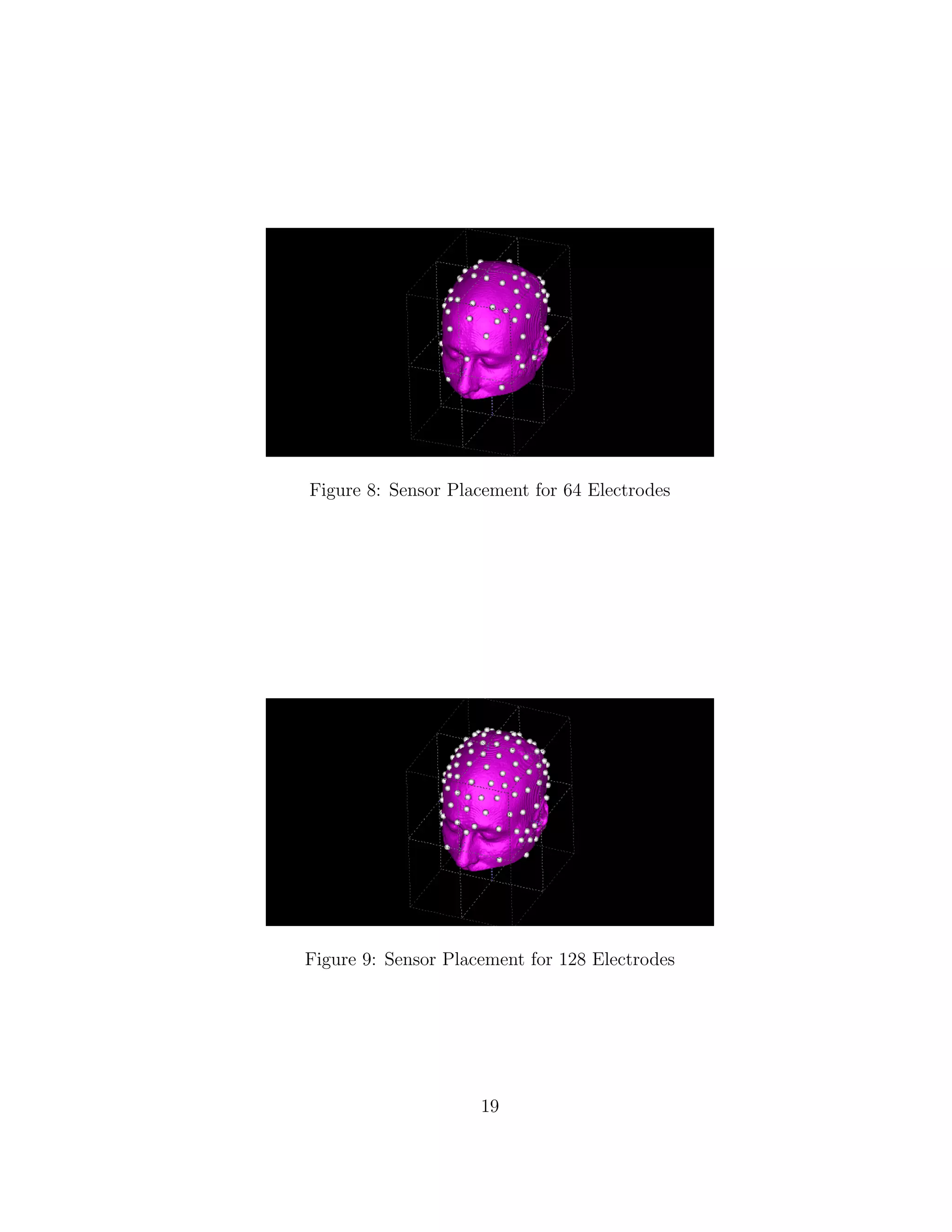
8 Sensor Placement for 64 Electrodes . . . . . . . . . . . . . . . . . 19
9 Sensor Placement for 128 Electrodes . . . . . . . . . . . . . . . . 19
10 Location Error With and Without Added Noise for Airhead 32-
30-30-4 . . . . . . . . . . . . . . . . . . . . . . . . . . . . . . . . 22
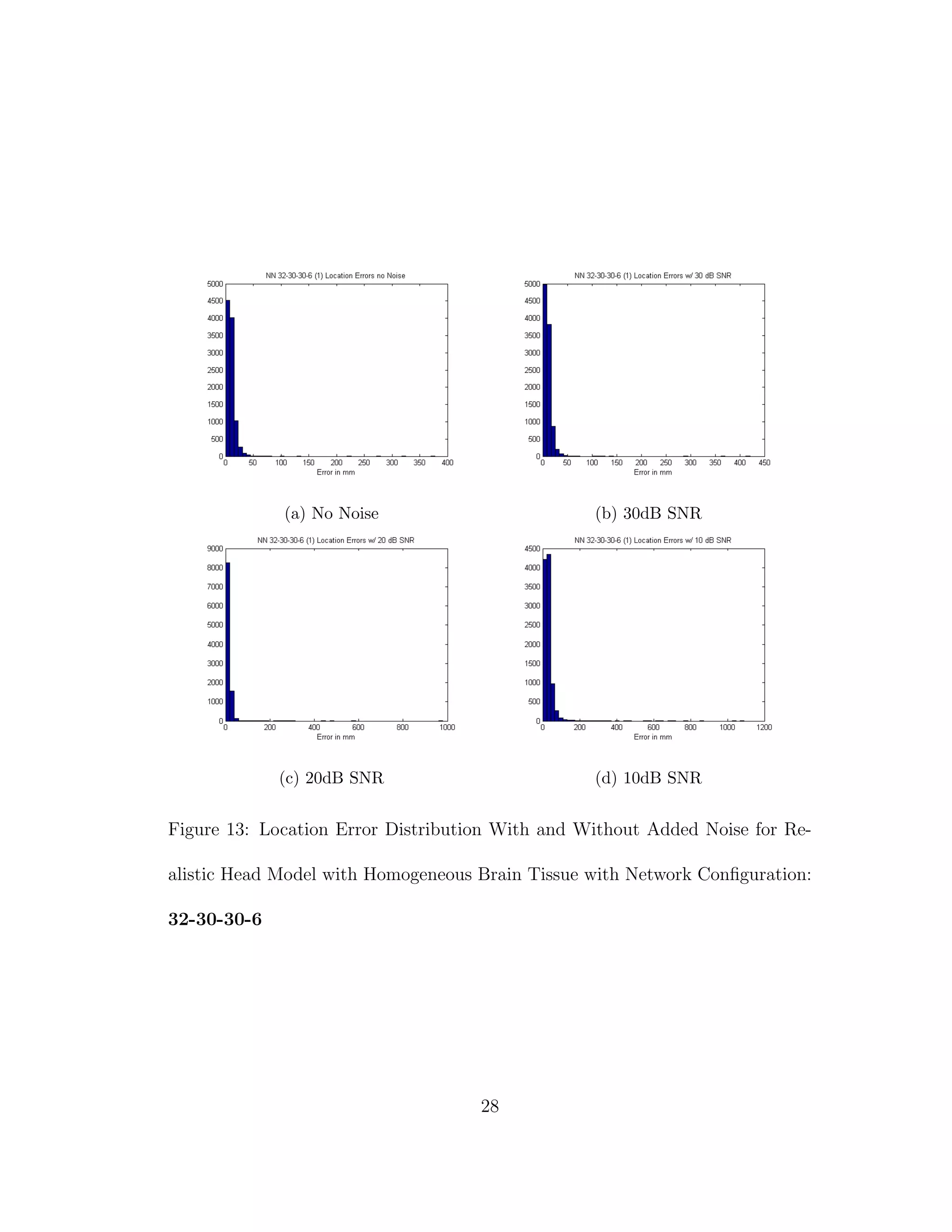
11 Location Error Distribution With and Without Added Noise for
2D Head Model with Network Configuration: 32-30-30-6 . . . . 23
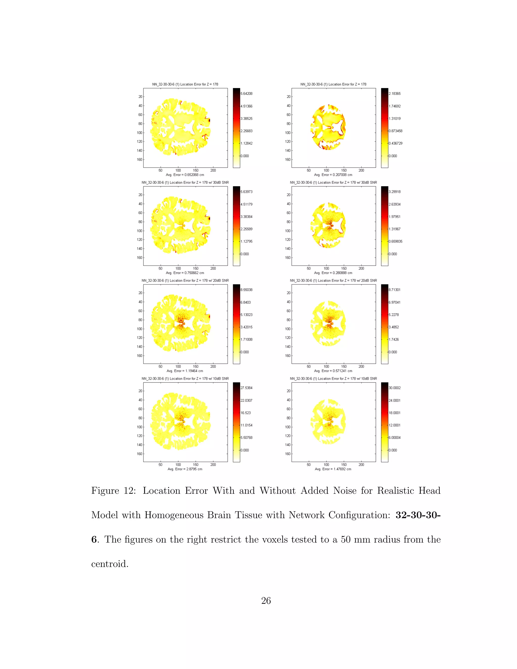
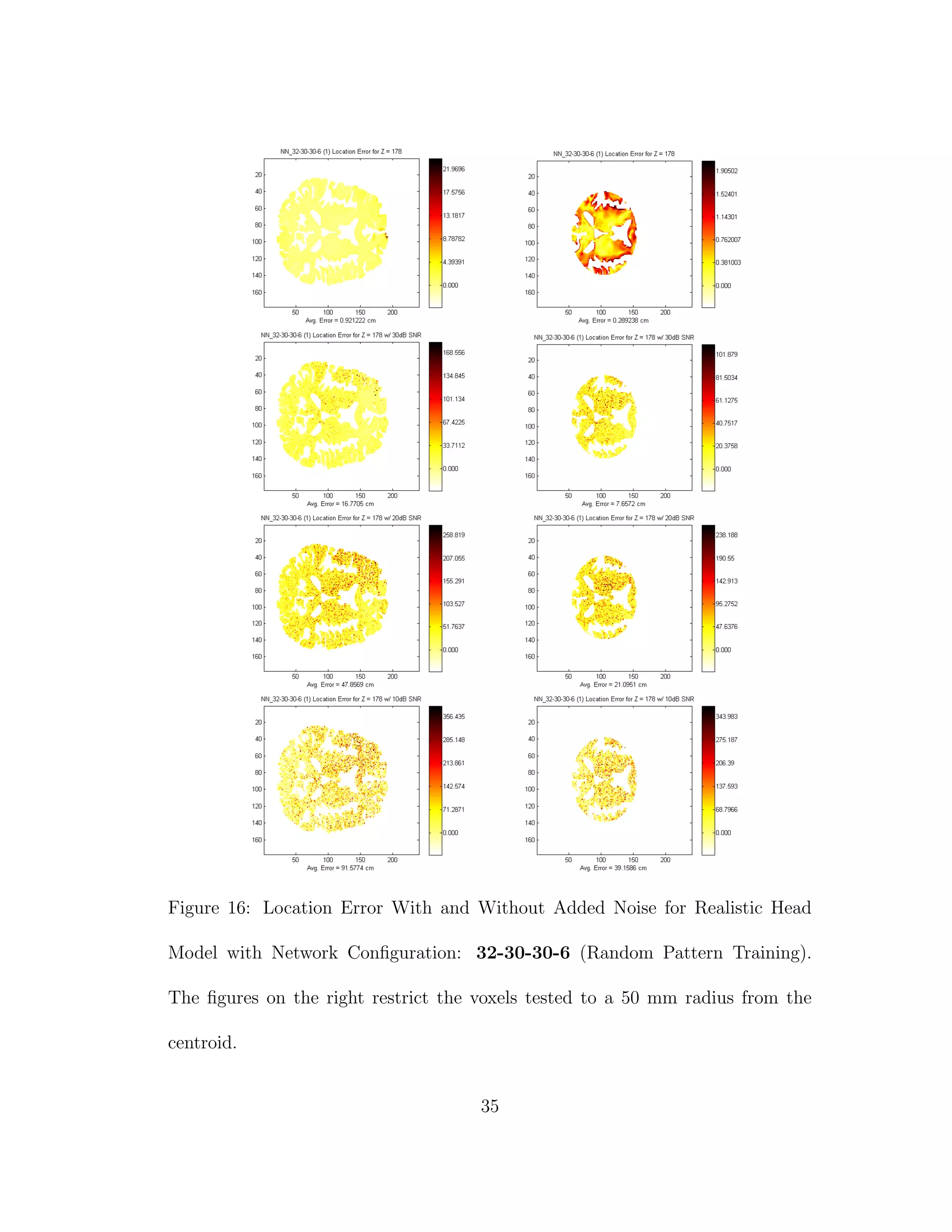
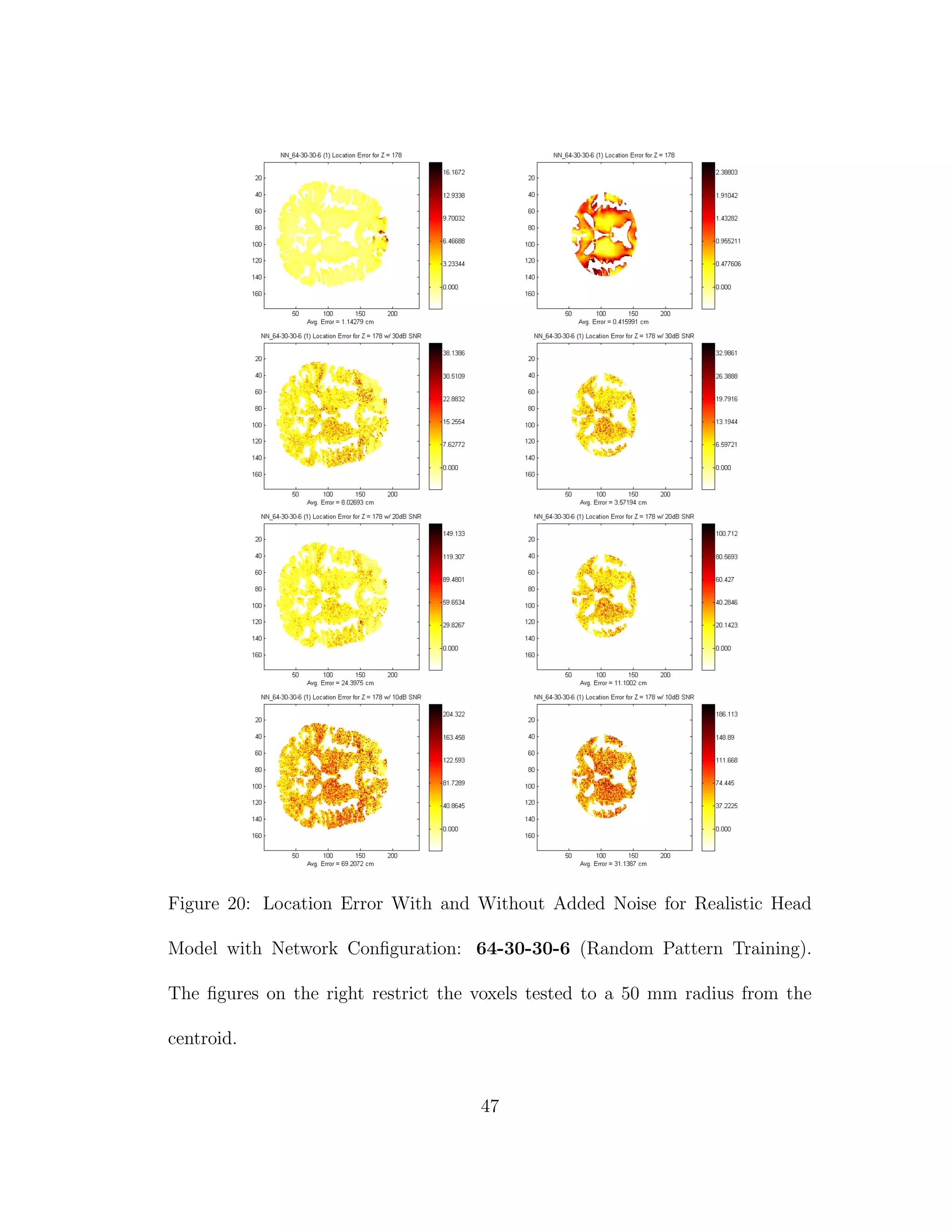
12 Location Error With and Without Added Noise for Realistic Head
Model with Homogeneous Brain Tissue with Network Configura-
tion: 32-30-30-6. The figures on the right restrict the voxels tested
to a 50 mm radius from the centroid. . . . . . . . . . . . . . . . . 26
xi

Realistic Head Model with Homogeneous Brain Tissue with Net-
work Configuration: 32-30-30-6 . . . . . . . . . . . . . . . . . . 28
Model with Network Configuration: 32-30-30-6 (Grid Pattern
Training). The figures on the right restrict the voxels tested to
a 50 mm radius from the centroid. . . . . . . . . . . . . . . . . . . 31
Realistic Head Model with Network Configuration: 32-30-30-6
(Grid Pattern Training) . . . . . . . . . . . . . . . . . . . . . . . 33
Model with Network Configuration: 32-30-30-6 (Random Pattern
Training). The figures on the right restrict the voxels tested to a
50 mm radius from the centroid. . . . . . . . . . . . . . . . . . . . 35
(Random Pattern Training) . . . . . . . . . . . . . . . . . . . . . 40
Training). The figures on the right restrict the voxels tested to
a 50 mm radius from the centroid. . . . . . . . . . . . . . . . . . . 43
xii

Model with Network Configuration: 64-30-30-6 (Random Pattern
Training). The figures on the right restrict the voxels tested to a
50 mm radius from the centroid. . . . . . . . . . . . . . . . . . . . 47
Training) The figures on the right restrict the voxels tested to a 50
mm radius from the centroid. . . . . . . . . . . . . . . . . . . . . 55
Model with Network Configuration: 128-30-30-6 (Random Pat-
tern Training). The figures on the right restrict the voxels tested
to a 50 mm radius from the centroid. . . . . . . . . . . . . . . . . 58
xiii

xiv

1 INTRODUCTION
The brain is widely recognized as the main controller of the human body. It
is also extremely hard to study without causing harm to the subject. Electroen-
cephalography (EEG) is a promising method for studying the way the brain works
using only passive means of observation. Unfortunately there is still the problem
of interpreting the data that we receive from EEG readings into accurate data
that we can use.
Source location is a significant problem due to the fact that it is ill posed.
Given a set of potentials for the electrodes there is an infinite number of possible
dipole strengths and locations that could have created this data set. There have
been many proposed solutions to this problem: iterative techniques, beamforming,
and artificial neural networks. Iterative techniques require immense amounts of
computations to arrive at their solutions and are not very robust to noise [2].
Beamformers have been shown to localize well with and without the presence of
noise [4], however they are still rather computationally intensive and are difficult
to impossible to perform in real time. Artificial neural networks (ANNs) could
provide us with a solution that is robust to noise [1][2][10][14][15] and can make
accurate location predictions fast enough to work in real time [10].
The ability to accurately detect brain activity location in real time could
lead to breakthroughs in psychology and thought activated devices. At the time of
1

writing I have only found one published article that tests artiﬁcial neural networks
with a realistic head model [10]. In said article the model was not as detailed as
models we could create today. While ANNs have been shown to be accurate
enough using simplistic head models, can an ANN show similar results if the head
is more complex, more closely related to our own heads?
2

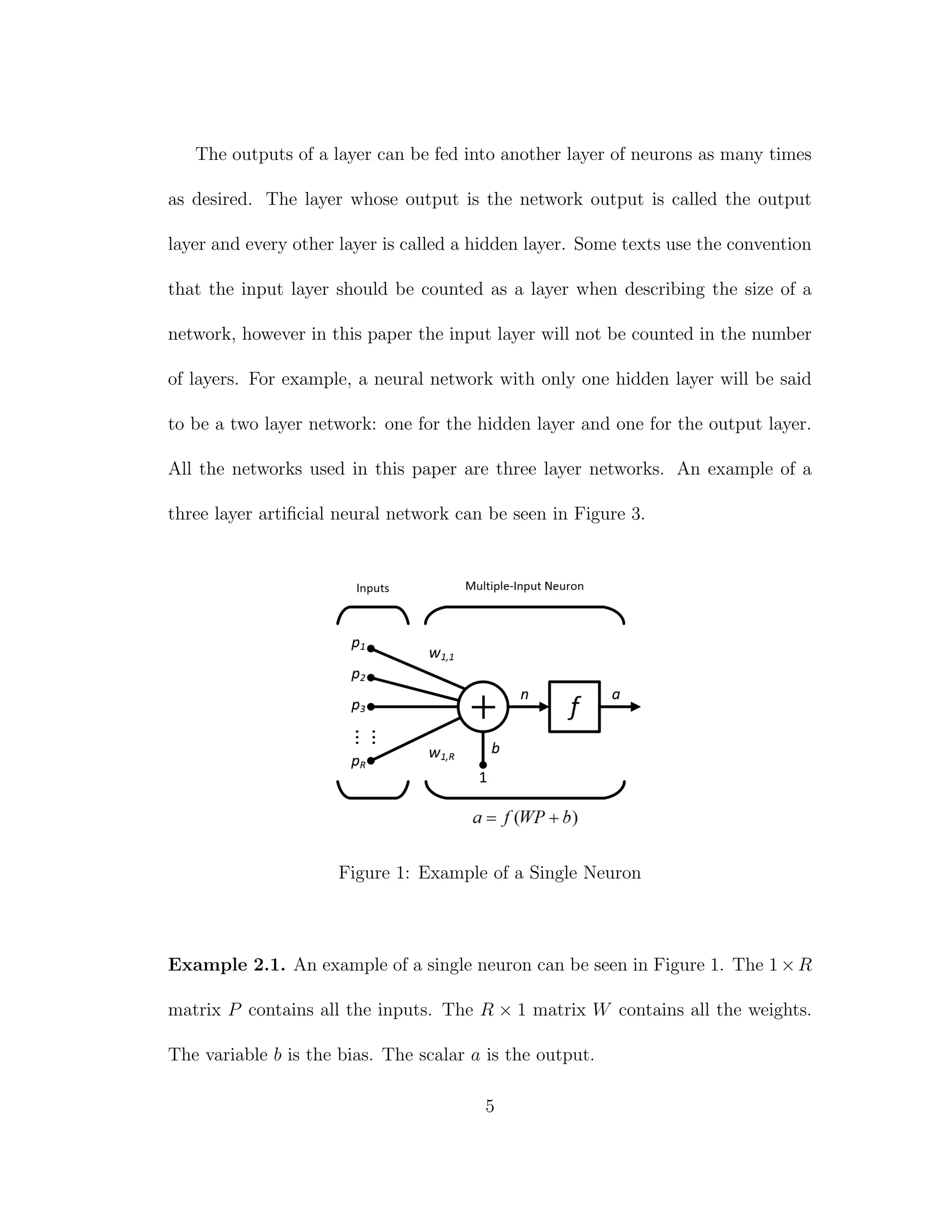
2 THEORY
This paper requires the knowledge of two subjects, the process for which the
forward solution was obtained, Finite Difference Neuroelectromagnetic Modeling
Software (FNS), and the process for which the inverse solution was obtained,
artificial neural networking.
2.1 FNS: Finite Difference Neuroelectromagnetic Modeling Software
The Finite Difference Neuroelectromagnetic Modeling Software (FNS) written
by Hung Dang [3] is a realistic head model EEG forward solution package. It
uses finite difference formulation for a general inhomogeneous anisotropic body
to obtain the system matrix equation, which is then solved using the conjugate
gradient algorithm. Reciprocity is then utilized to limit the number of solutions
to a manageable level.
This software attempts to solve the Poisson equation that governs electric
potential φ:
· (σ φ) = · Ji (1)
where σ is the conductivity and Ji is the impressed current density. It accom-
plishes this using the finite difference approximation for the Laplacian:
3

· (σ φ)
node0
≈
6
i=1
Aiφi −
6
i=1
Ai φ0 (2)
where φi is the potential at node i, and the coefficients Ai depend on conductivities
of the elements and node spacings.
2.2 Artificial Neural Networks
Biological nervous systems are capable of learning and replicating extremely
complex tasks. Artificial neural networks are mathematical models designed to
imitate these biological systems. They are attractive, because they are capable
of establishing input/output relationships with only training data and no prior
knowledge of the system.
An artificial neural network is nothing more than an inter-connected col-
lection of neurons. Each neuron consists of one or more weighted inputs and a bias
that are summed together. This value is then passed through a transfer function.
The transfer function is chosen to satisfy some specification of the problem and
may be linear or nonlinear. Neurons are then organized into layers. A typical
layer contains several neurons that all have the same inputs, however the weights
for these inputs are usually different for each neuron and input. The output for
each layer can be written:
am+1
= fm+1
(Wm+1
am
+ bm+1
) for m = 0, 1, ..., M − 1,
4

The outputs of a layer can be fed into another layer of neurons as many times
as desired. The layer whose output is the network output is called the output
layer and every other layer is called a hidden layer. Some texts use the convention
that the input layer should be counted as a layer when describing the size of a
network, however in this paper the input layer will not be counted in the number
of layers. For example, a neural network with only one hidden layer will be said
to be a two layer network: one for the hidden layer and one for the output layer.
All the networks used in this paper are three layer networks. An example of a
three layer artiﬁcial neural network can be seen in Figure 3.
Figure 1: Example of a Single Neuron
Example 2.1. An example of a single neuron can be seen in Figure 1. The 1×R
matrix P contains all the inputs. The R × 1 matrix W contains all the weights.
The variable b is the bias. The scalar a is the output.
5

Figure 2: Example of a Single Layer of Neurons
Example 2.2. An example of a single layer of neurons can be seen in Figure 2.
The input matrix P remains a 1 × R matrix, however the weight matrix becomes
an R × S matrix where S is the number of neurons in the layer. This is because
even though each neuron receives the same inputs, the weight applied to each
input is different for each neuron/input combination. The 1 × S matrix, A, is the
output.
Example 2.3. An example of a three layer multi-input/multi-output artificial
neural network can be seen in Figure 3. As you can see the outputs from one
layer become the inputs for the next layer. The final equation that ties the input
6

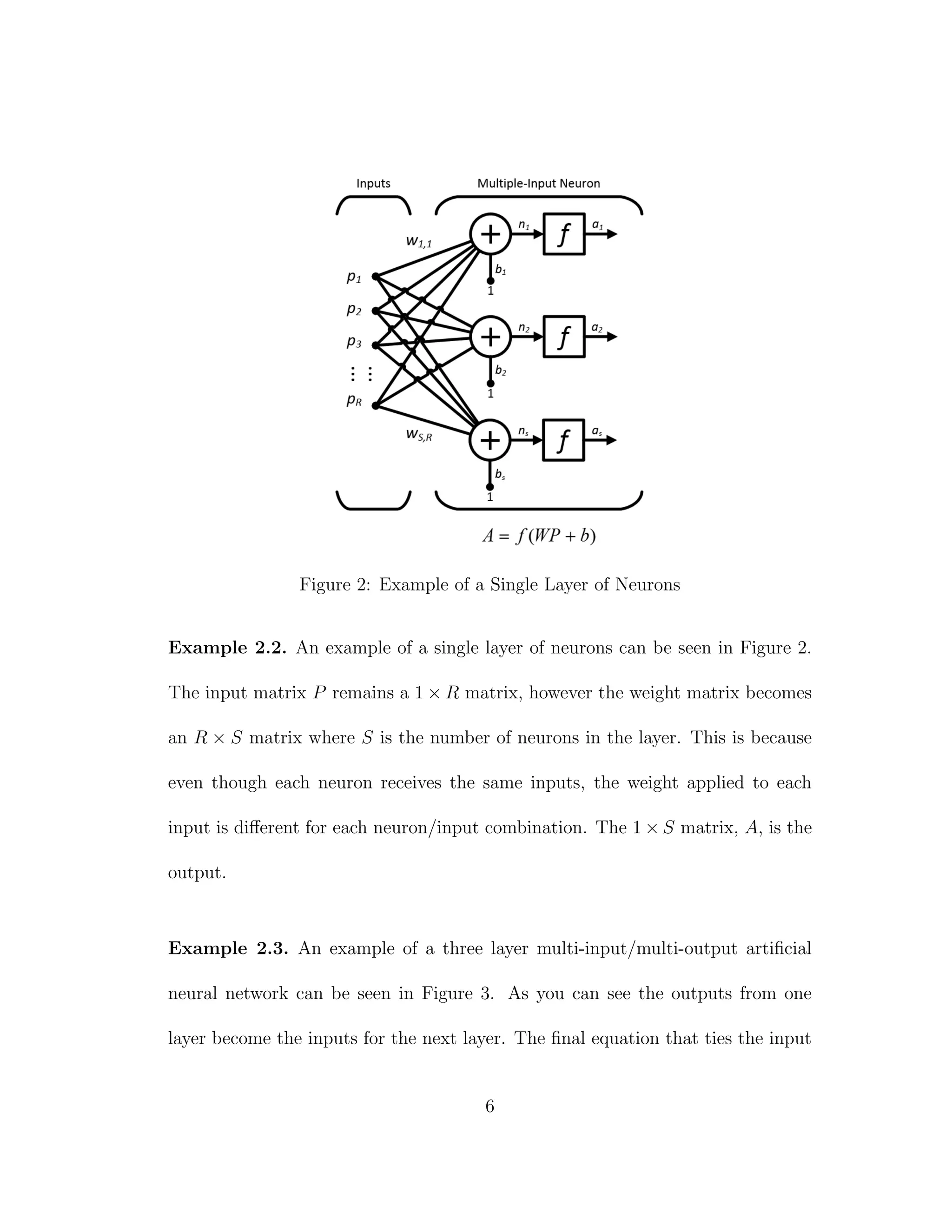
Figure 3: Example of a Three Layer of Neural Network
matrix, P, to the output matrix, A3
, is
A3
= f3
(W3
f2
(W2
f1
(W1
P + b1
) + b2
) + b3
)
2.2.1 Backpropagation
The best part about neural networks is their ability to replicate complex sys-
tems with only knowing input-output combinations. There are basically two ways
for a network to do this, supervised and unsupervised learning. For this paper we
will focus on supervised learning. The most common form of supervised learning
is the backpropagation method [1]. The backpropagation method uses calculus’
Chain Rule to propagate the mean square error of an input-output pair back
7

through a network. Weights and biases are then updated such that the mean
square error is reduced.
Deﬁnition 2.1. The basic algorithm for the back propagation method is as fol-
lows:
A0
= P (3)
Am+1
= fm+1
(Wm+1
Am
+ bm+1
) for m = 0, 1, ..., M − 1 (4)
O = AM
(5)
sM
= −2 ˙FM
(nM
)(T − O) (6)
sm
= ˙Fm
(nm
)(Wm+1
) sm+1
, for m = M − 1, ..., 2, 1 (7)
Wm
(k + 1) = Wm
(k) − αsm
(Am−1
) (8)
bm
(k + 1) = bm
(k) − αsm
(9)
where T is the target vector, O is the output vector, P is the input vector, W is
the weight matrix, b is the bias matrix, and α is the learning rate. Generally the
learning rate is set to a very low number (e.g., α = 0.1 or 0.01).
2.2.2 Levenberg-Marquardt Backpropagation
All the networks in this paper were trained using the Levenberg-Marquardt
backpropagation algorithm. “The Levenberg-Marquardt algorithm is a variation
8

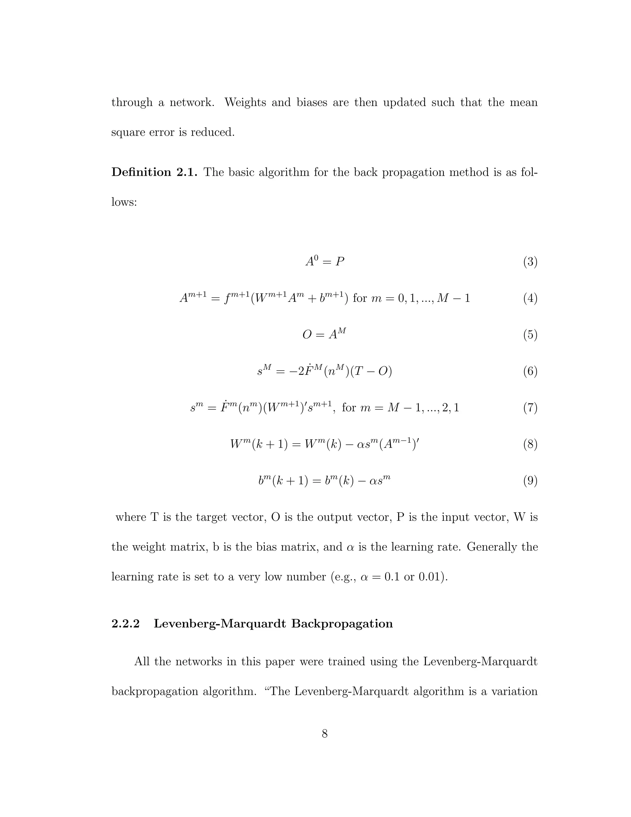
of Newton’s method that was designed for minimizing functions that are sums of
squares of other nonlinear functions” [5]. It is a batch learning algorithm that
can adjust its learning rate in order to ﬁnd the best weights and biases in the
fewest number of iterations. The main problem with this method is the extreme
memory requirement with larger networks. For example Matlab required around
40 gigabytes of virtual memory during the training of each of the 128-30-30-6
networks discussed in this paper.
Deﬁnition 2.2. The Levenberg-Marquardt backpropagation algorithm is as fol-
lows:
1. For Q input-output pairs, run all inputs through the network to obtain the
errors, Eq = Tq − AM
q . Then determine the sum of squared errors over all
inputs, F(x).
F(x) =
Q
q=1
(Tq − Aq) (Tq − Aq) (10)
9

2. Determine the Jacobian matrix:
J(x) =























∂e1,1
∂w1
1,1
∂e1,1
∂w1
1,2
· · ·
∂e1,1
∂w1
S1,R
∂e1,1
∂b1
1
· · ·
∂e2,1
∂w1
1,1
∂e2,1
∂w1
1,2
· · ·
∂e2,1
∂w1
S1,R
∂e2,1
∂b1
1
· · ·
...
...
...
...
∂eSM ,1
∂w1
1,1
∂eSM ,1
∂w1
1,2
· · ·
∂eSM ,1
∂w1
S1,R
∂eSM ,1
∂b1
1
· · ·
∂e1,2
∂w1
1,1
∂e1,2
∂w1
1,2
· · ·
∂e1,2
∂w1
S1,R
∂e1,2
∂b1
1
· · ·
...
...
...
...























(11)
Calculate the sensitivities:
˜sm
i,h ≡
∂vh
∂nm
i,q
=
∂ek,q
∂nm
i,q
(Marquardt Sensitivity) where h = (q−1)SM
+k (12)
˜SM
q = − ˙FM
(nM
q ) (13)
˜Sm
q = ˙F(nm
q )(Wm+1
) ˜Sm+1
q (14)
˜Sm
= ˜Sm
1
˜Sm
2 · · · ˜Sm
Q
(15)
And compute the elements of the Jacobian matrix:
[J]h,l =
∂vh
∂xl
=
∂ek,q
∂wm
i,j
=
∂ek,q
∂nm
i,q
×
∂nm
i,q
∂wm
i,j
= ˜sm
i,h ×
∂nm
i,q
∂wm
i,j
= ˜sm
i,h × am−1
j,q
for weight xl (16)
[J]h,l =
∂vh
∂xl
=
∂ek,q
∂bm
i
=
∂ek,q
∂nm
i,q
×
∂nm
i,q
∂bm
i
= ˜sm
i,h ×
∂nm
i,q
∂bm
i
= ˜sm
i,h
for bias xl (17)
10

Where:
v = v1 v2 · · · vN
= e1,1 e2,1 · · · eSM ,1 e1,2 · · · eSM ,Q
(18)
x = x1 x2 · · · xN
= w1
1,1 w1
1,2 · · · w1
S1,R b1
1 · · · b1
S1 w2
1,1 · · · bM
SM
(19)
3. Solve:
∆xk = −[J (xk)J(xk) + µkI]−1
J (xk)v(xk) (20)
4. Compute F(x), Eq (10), using xk + ∆xk. If the result is less than the
previous F(x) divide µ by ϑ, let xk+1 = xk + ∆xk and go back to step 1. If
not, multiply µ by ϑ and go back to step 3. The variable, ϑ, must be greater
than 1 (e.g., ϑ = 10).
11

3 APPROACH
The first step to testing out an artificial neural network on a complex realistic
head model was to test on a simplistic homogeneous model and compare the results
to published findings. The next step was to train and test an ANN for a realistic
head model with less complex conductivities. Finally, I trained and tested several
ANNs for a complex realistic head model. Every network is trained to output
location coordinates and a moment vector. The moment vector is essentially the
direction of the dipole. Both the location and moment vector errors are determined
the same way in this paper:
Error = (x − x )2 + (y − y )2 + (z − z )2 (21)
where (x, y, z) and (x , y , z ) are the network estimated values and the actual
values respectively. For the 2D headmodel the z and z terms are equal to zero.
3.1 2D Headmodel
For this step a simple homogeneous circular two dimensional model needed
to be defined. In order to make it similar to an actual human head two regions
are required: the brain area and the scalp area. The brain area would be the area
where dipoles could be present. The scalp area would be where the sensors could
pick up the potentials created by the dipoles. The brain area was determined to
12

have a radius of 6.7 cm. The scalp area was determined to have a radius of 8 cm.
The resolution was determined to be 1 mm × 1 mm. If we consider the entirety
of both circles to be ﬁlled with only air the equation to determine the potential
at a given sensor point from a dipole would be:
V =
( ˆds) · ( ¯R − ¯R )
| ¯R − ¯R |3
, where s =
qd
4π 0
or
Id
4πσ
(22)
Example 3.1. A visual representations of this “airhead” can be seen in Figure 4.
In this case the dipole has been placed at X = 90 and Y = 100. The dipole is X
directed. This graphic shows the potential from the dipole at every point in the
brain circle and on the outer scalp circle. The potentials on the scalp have been
multiplied by a factor of 10 in order to make the colors distinguishable.
Figure 4: Example of a Single Dipole in a 2D Airhead Model
Thirty-two scalp nodes were chosen semi-randomly to be the sensor loca-
13

tions. Training points were determined by choosing dipole locations in a grid
format with a resolution of 5 mm × 5 mm. All training locations and sensor
locations can be seen in Figure 5. This resulted in 567 training locations. Sensor
values were obtained for each of these locations in all four of the cardinal direc-
tions, +X, −X, +Y , and −Y , resulting in 2,268 total training input-output pairs.
Each of these input-output pairs were presented to a 32-30-30-4 network to train.
Figure 5: Sensor and Training Dipole Locations for 2D Homogeneous Head Model
Once trained our network was subjected to multiple tests. Our ultimate
goal was to test accuracy, so the ﬁrst test was for each possible dipole location to
set the direction of the dipole to face +X and determine how accurate the network
could determine its actual location and direction. Then noise was added such
that SNR = 10 dB, 20 dB, and 30 dB. Then the tests were conducted with 10,000
dipoles with random location and direction. This case is used to characterize the
14

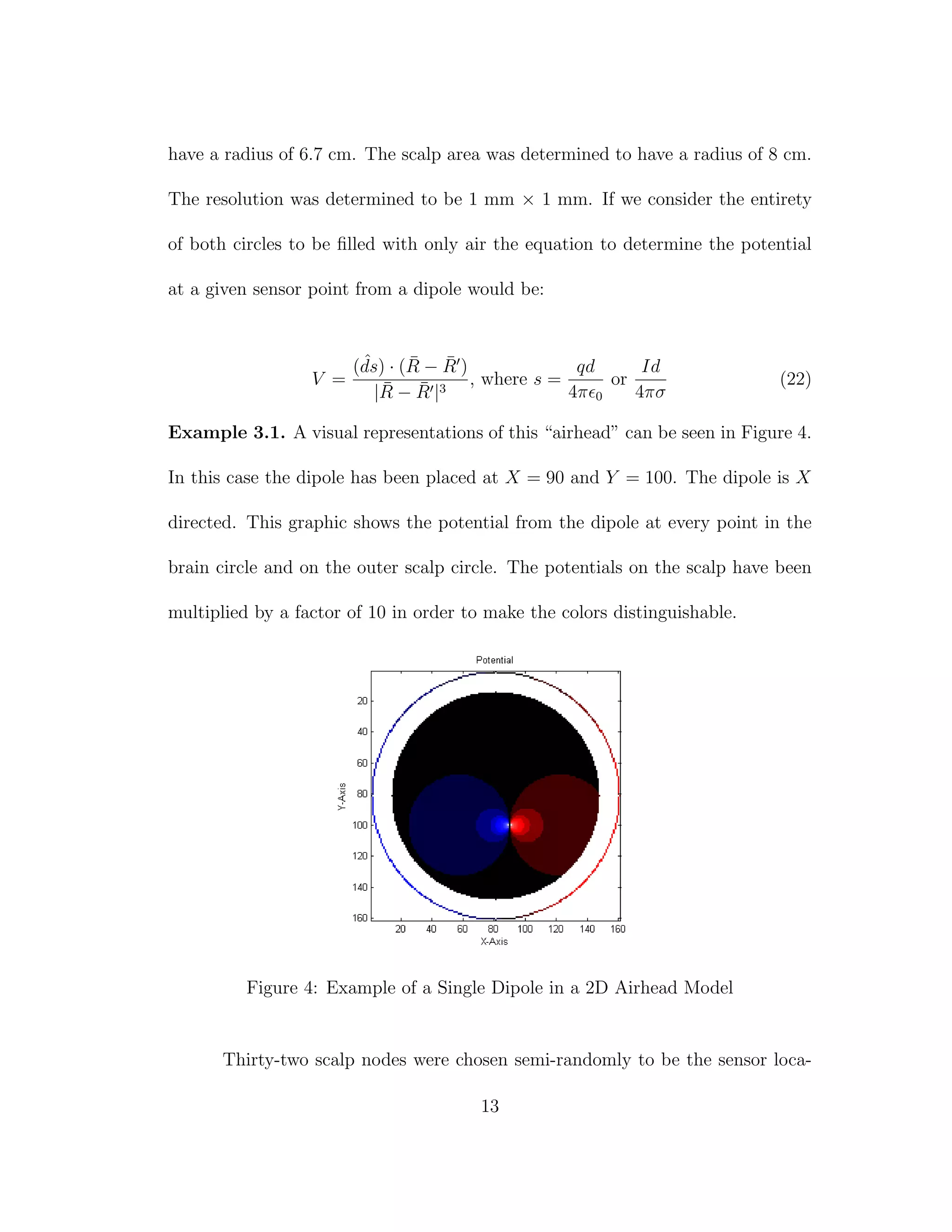
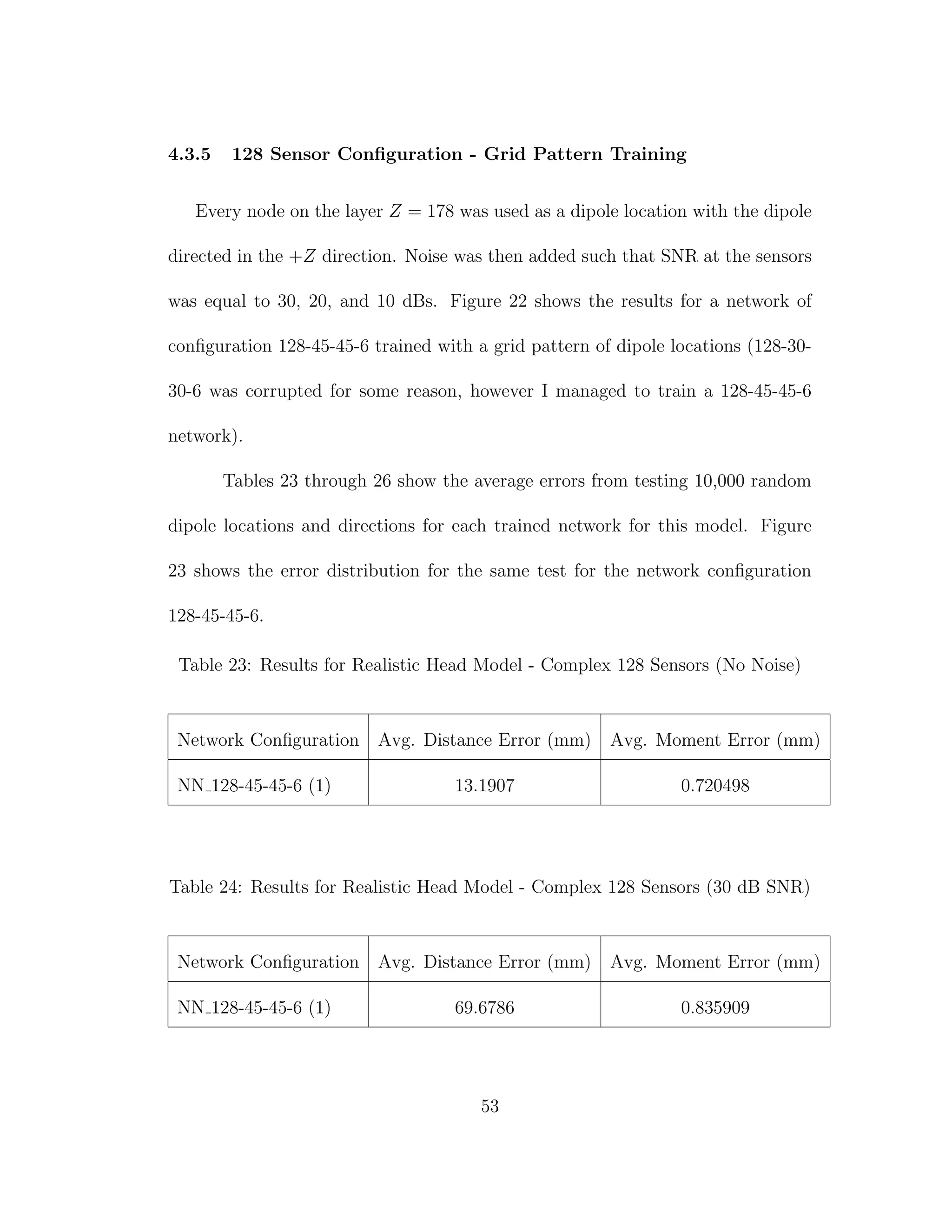
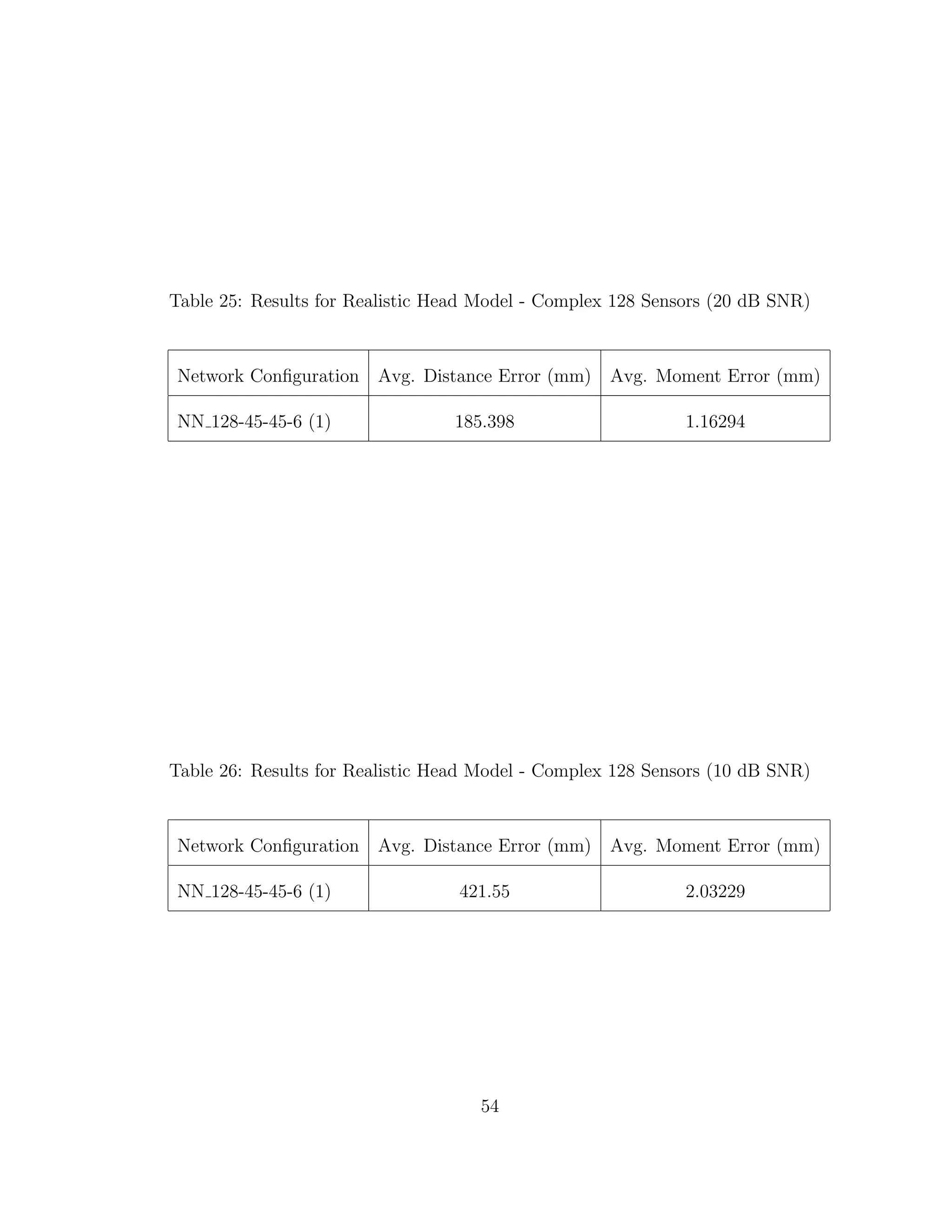
general accuracy of the network. In all cases each dipole was required to have the
same magnitude.
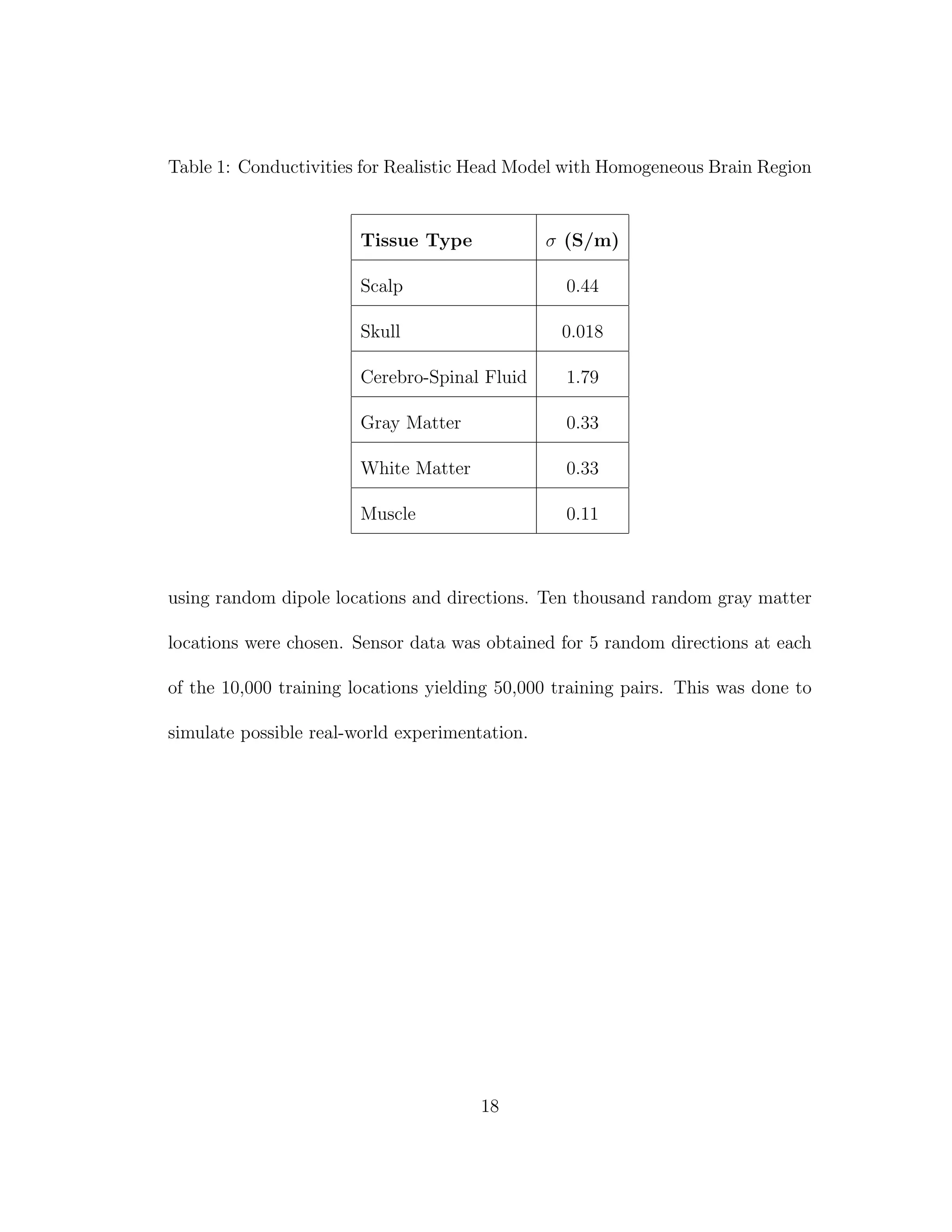
3.2 Realistic Head Model - Homogeneous Brain Region
In order to create a truly realistic head model we must start with an FMRI
image such as can be seen in Figure 6. The FMRI image used had a resolution of
1 mm × 1 mm × 1 mm. The image was segmented using the program, FSL [6].
The segmented image was then fed into FNS [3] to obtain the reciprocity data
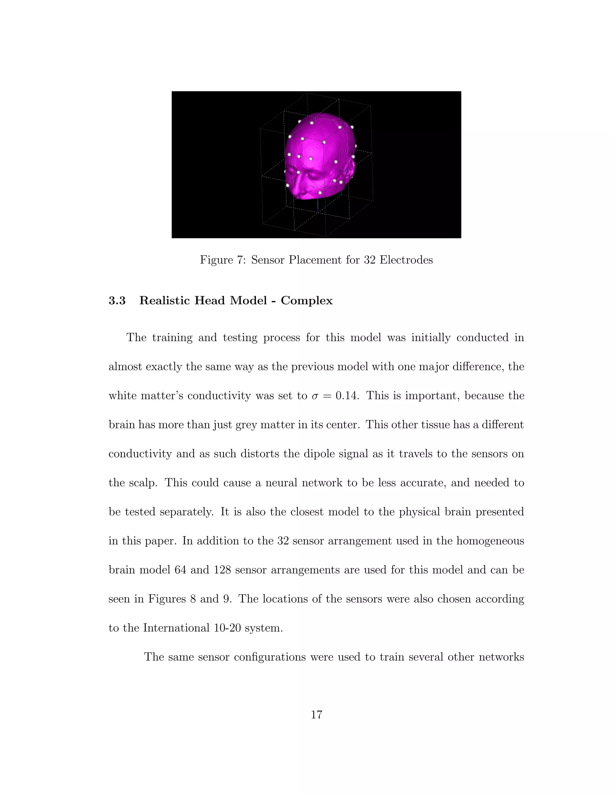
for all possible dipole locations at the chosen sensor locations. Sensor locations
were chosen according to the International 10-20 system for 32 electrodes. The
placement of these sensors can be seen in Figure 7. In order to make the brain
area homogeneous the conductivity of the white matter was changed to that of
grey matter. The conductivities can be seen in Table 1.
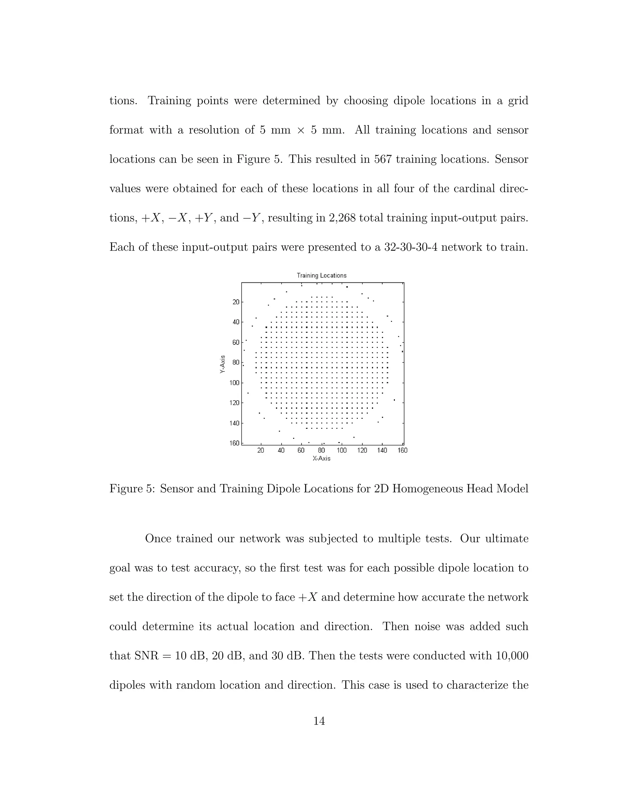
Once the reciprocity data had been obtained training dipole locations and
directions were chosen. Training locations were chosen in a grid format with a
resolution of 5 mm × 5 mm × 5 mm. Training directions were chosen as +X,
−X, +Y , −Y , +Z, −Z, and 4 other random directions. Because dipoles could
only occur in grey matter this yielded 100,340 diﬀerent input-output pairs. These
training pairs were then presented to the networks for training.
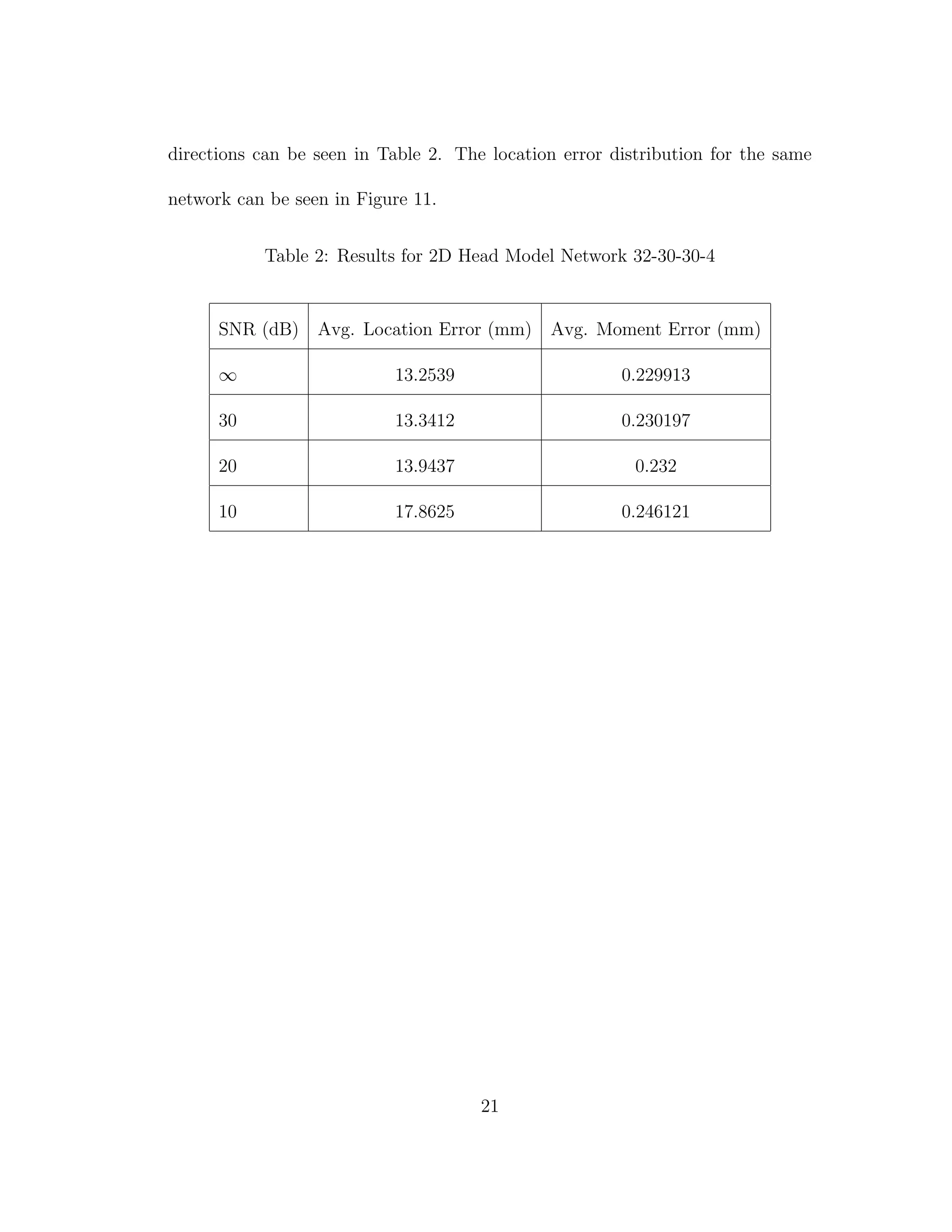
Once the networks were trained the sensor data from 10,000 dipoles with
random locations and directions were presented to the network. The average
15

Figure 6: FMRI Image Used for Realistic Head Model (ITK-SNAP [13])
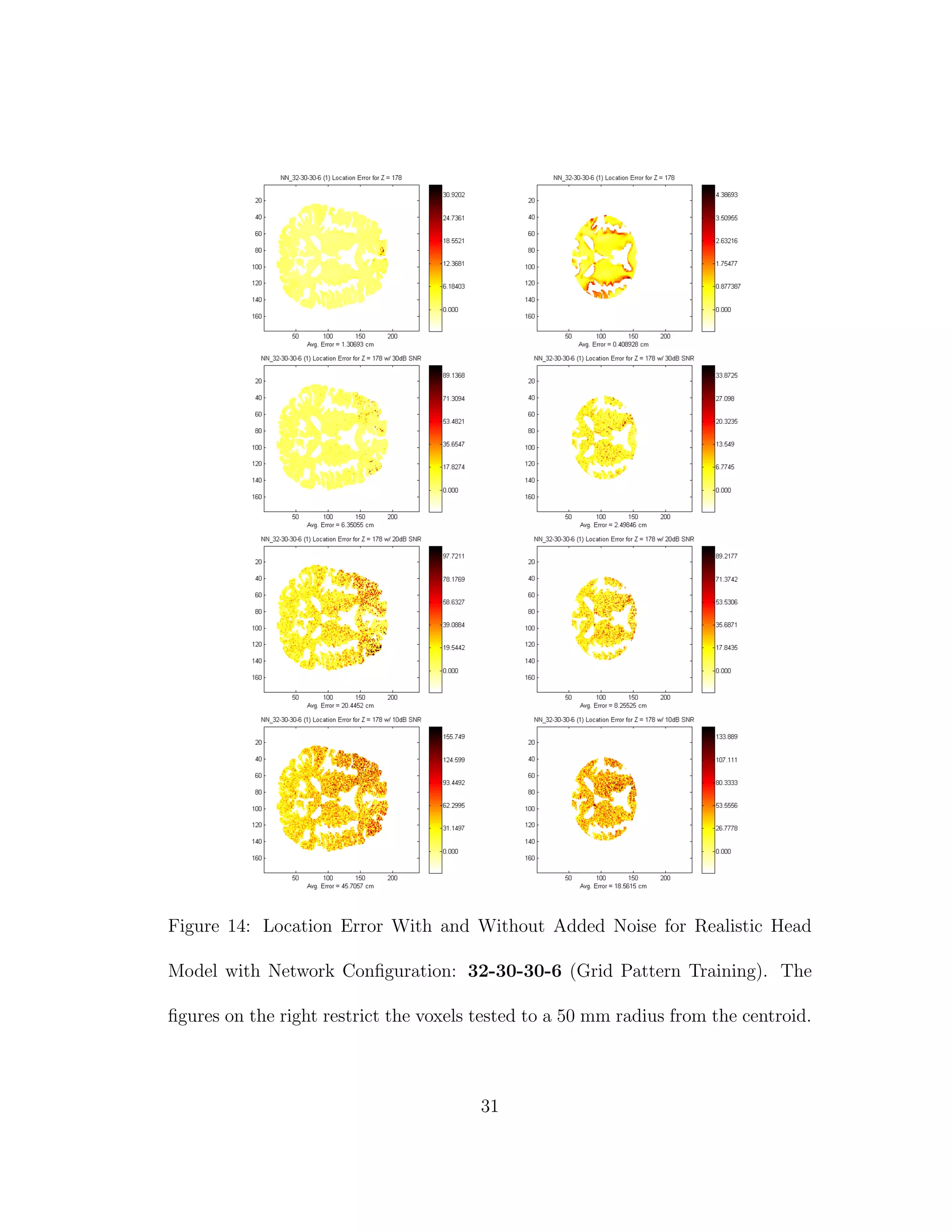
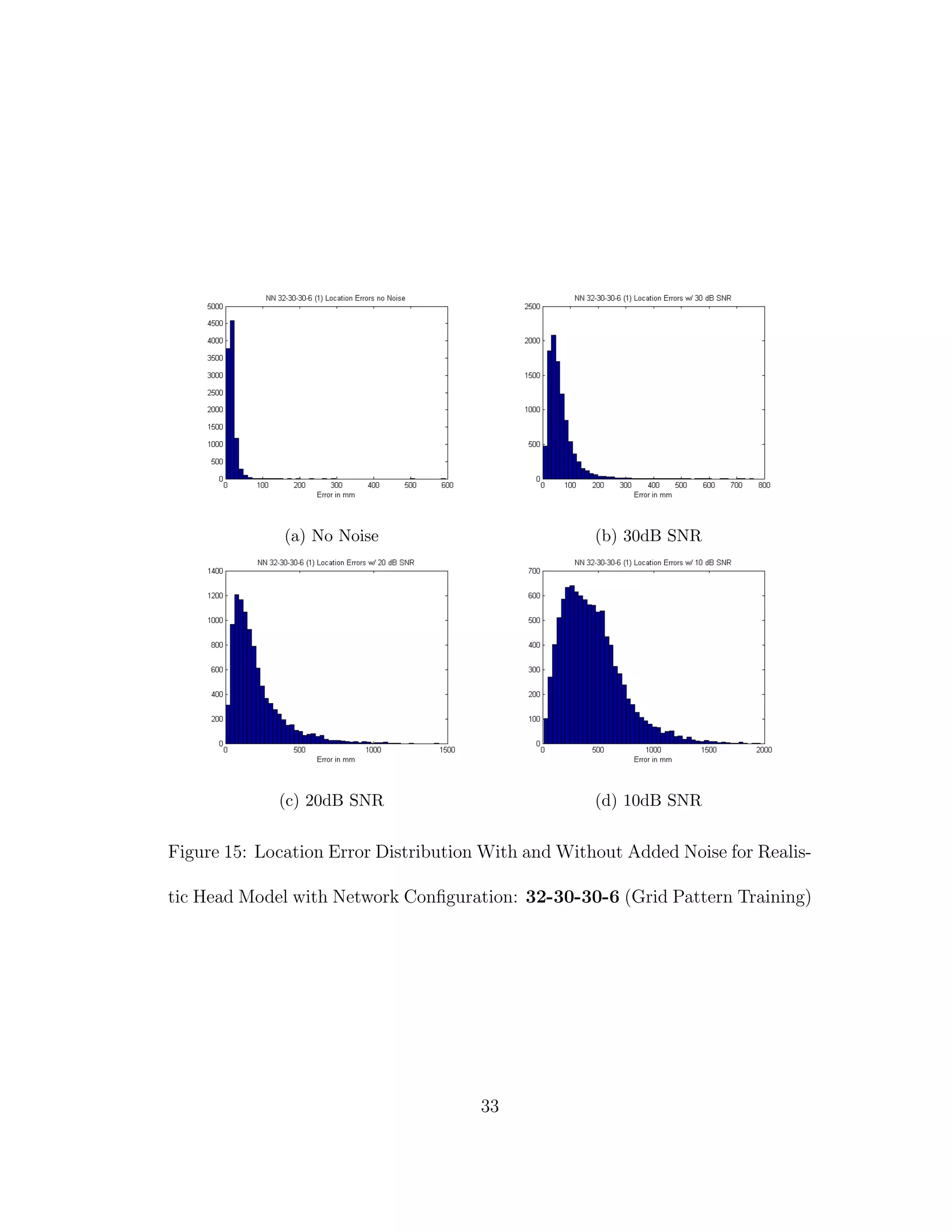
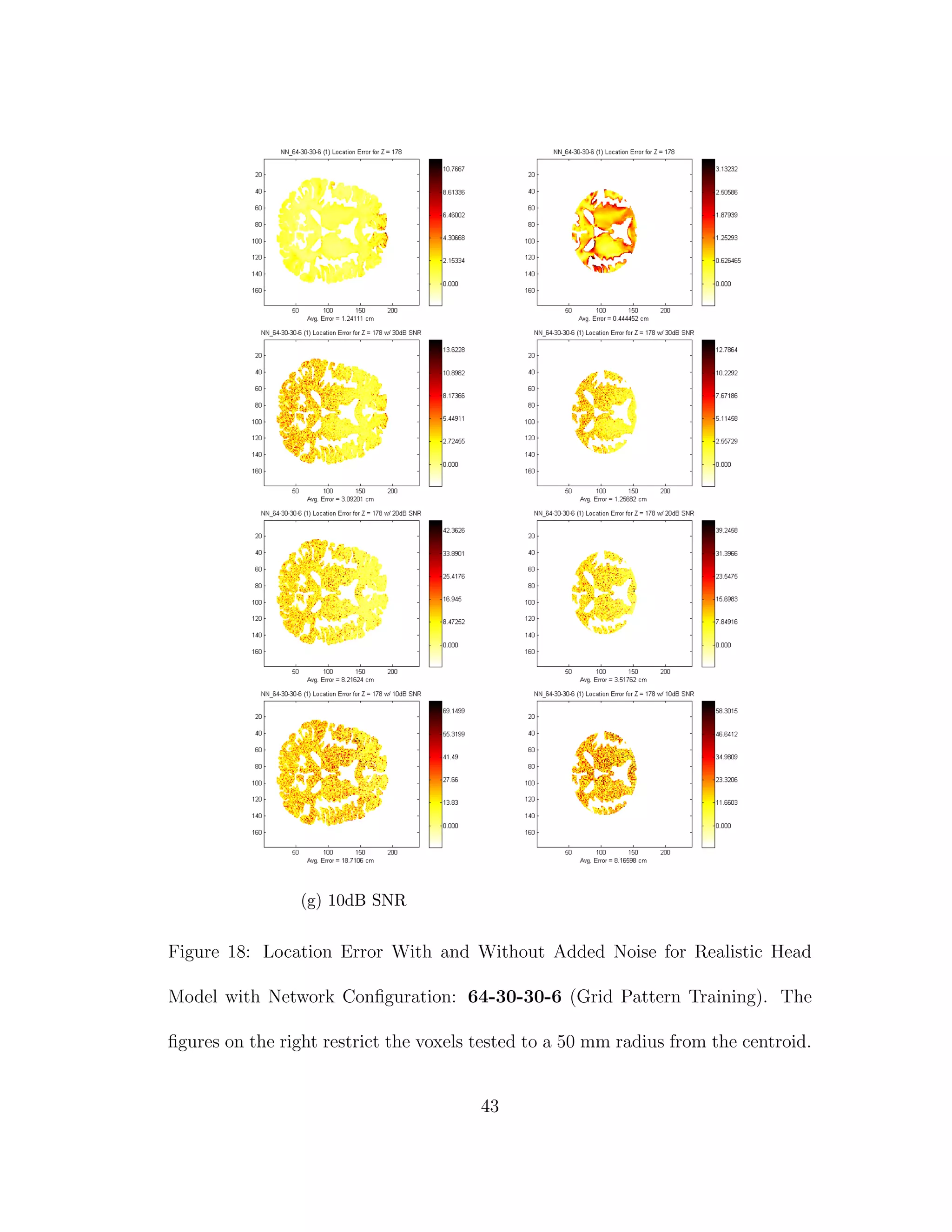
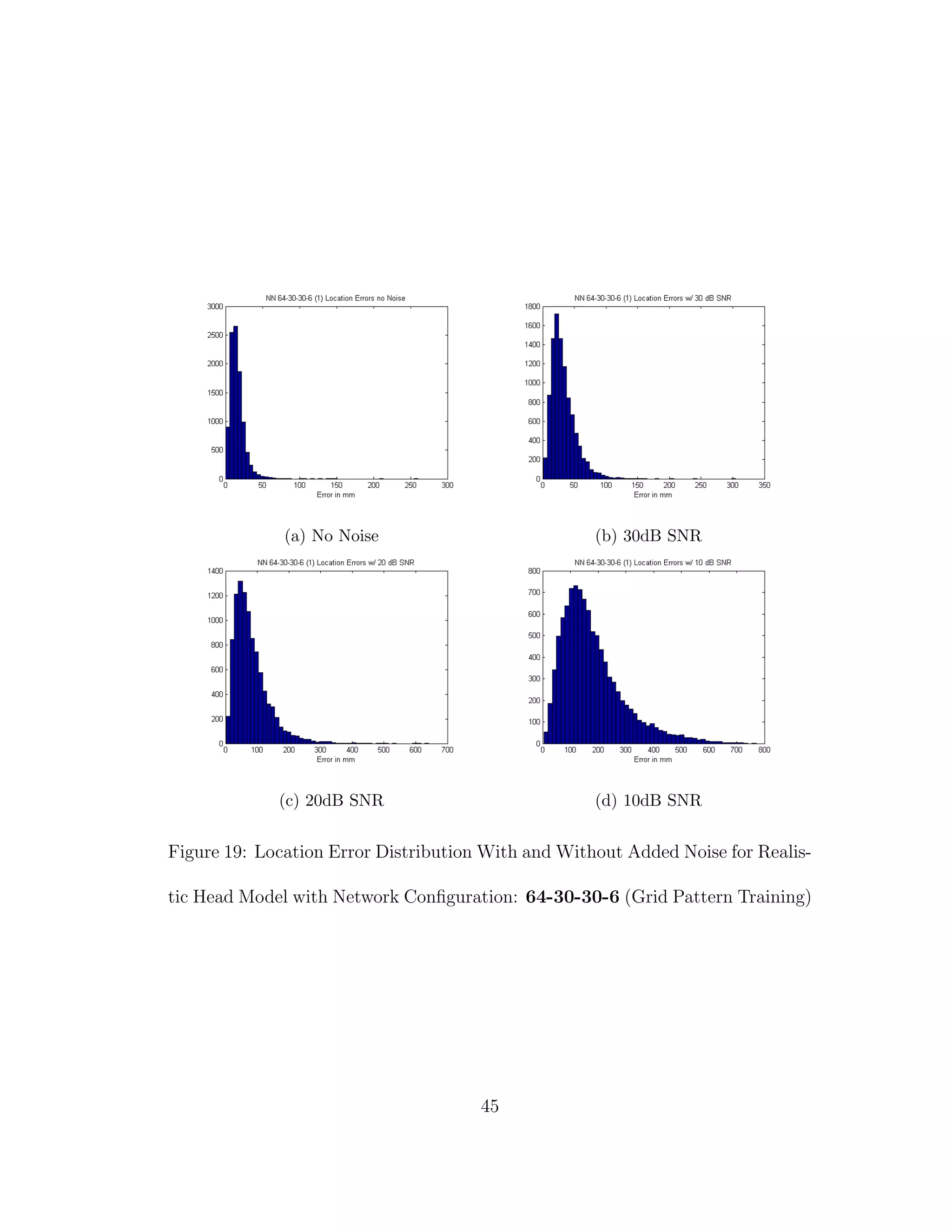
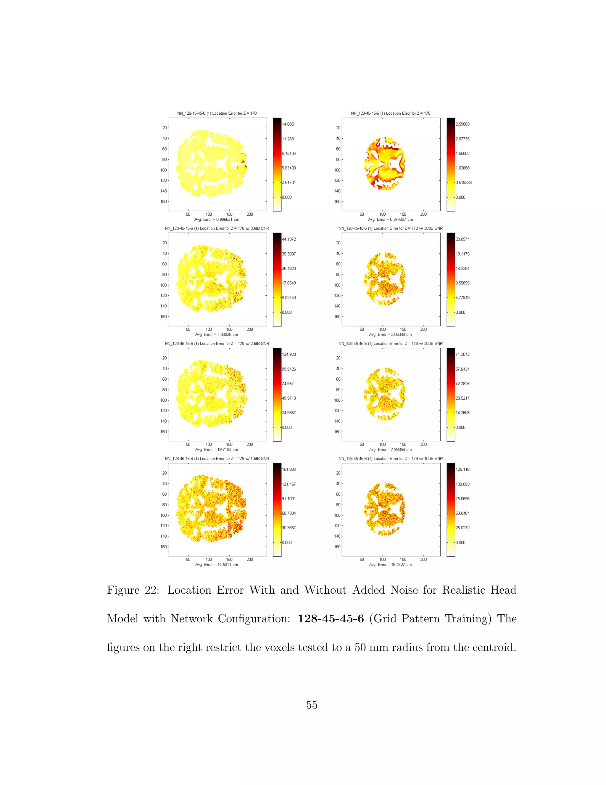
location and direction errors were recorded. Next every grey matter node where
Z = 178 was used as a dipole location with direction +Z. Layer Z = 178 was
chosen because it is a thick area of the brain near the center of mass. The average
location and direction errors are recorded. Noise is then introduced such that
SNR = 10 dB, 20 dB, and 30 dB. The same tests are performed again for any
voxels within 55 mm of the centroid of the layer. This is done, because it has
been noted that neural networks tend to have larger errors when source locating
near the boundary of the training area and would have better average accuracy
near the centroid of the training area [10].
16

Figure 7: Sensor Placement for 32 Electrodes
3.3 Realistic Head Model - Complex
The training and testing process for this model was initially conducted in
almost exactly the same way as the previous model with one major difference, the
white matter’s conductivity was set to σ = 0.14. This is important, because the
brain has more than just grey matter in its center. This other tissue has a different
conductivity and as such distorts the dipole signal as it travels to the sensors on
the scalp. This could cause a neural network to be less accurate, and needed to
be tested separately. It is also the closest model to the physical brain presented
in this paper. In addition to the 32 sensor arrangement used in the homogeneous
brain model 64 and 128 sensor arrangements are used for this model and can be
seen in Figures 8 and 9. The locations of the sensors were also chosen according
to the International 10-20 system.
The same sensor configurations were used to train several other networks
17

Table 1: Conductivities for Realistic Head Model with Homogeneous Brain Region
Tissue Type σ (S/m)
Scalp 0.44
Skull 0.018
Cerebro-Spinal Fluid 1.79
Gray Matter 0.33
White Matter 0.33
Muscle 0.11
using random dipole locations and directions. Ten thousand random gray matter
locations were chosen. Sensor data was obtained for 5 random directions at each
of the 10,000 training locations yielding 50,000 training pairs. This was done to
simulate possible real-world experimentation.
18

19

4 RESULTS
This section details the results obtained from the tests described in the Ap-
proach section.
4.1 2D Head Model
Figure 10 visually shows the results from a 32-30-30-4 artificial neural network
trained to detect the locations of a single dipole present in a circular airhead as
described in the Approach section. As you can see from the two figures that had no
noise introduced to them the average error is less than a millimeter or one voxel
in this case. This means that the network is exactly right in most cases when
it comes to predicting location. As we add noise to the signals received by the
sensors we can see the accuracy drop off as we would expect it to. It is interesting
to note that in every case the network is more error prone as the dipole is moved
toward the edge of the training region away from the center. This is shown by
the left images containing all the voxels from our airhead and the right images
containing only those voxels within 55 mm of the center of the airhead. This is
a normal trait of artificial neural networks. It is also interesting to note that the
accuracy is not uniform throughout the no noise cases. This is due to the random
starting weights and biases for each network.
The average location and moment errors from 10,000 random locations and
20

directions can be seen in Table 2. The location error distribution for the same
network can be seen in Figure 11.
Table 2: Results for 2D Head Model Network 32-30-30-4
SNR (dB) Avg. Location Error (mm) Avg. Moment Error (mm)
∞ 13.2539 0.229913
30 13.3412 0.230197
20 13.9437 0.232
10 17.8625 0.246121
21

(a) No Noise (b) No Noise, 55mm Radius
(c) 30dB SNR (d) 30dB SNR, 55mm Radius
(e) 20dB SNR (f) 20dB SNR, 55mm Radius
(g) 20dB SNR (h) 20dB SNR, 55mm Radius
Figure 10: Location Error With and Without Added Noise for Airhead 32-30-
30-4
22

(a) No Noise (b) 30dB SNR
(c) 20dB SNR (d) 10dB SNR
Figure 11: Location Error Distribution With and Without Added Noise for 2D
Head Model with Network Conﬁguration: 32-30-30-6
23

4.2 Realistic Head Model - Homogeneous Brain Region
Every node on the layer Z = 178 was used as a dipole location with the dipole
directed in the +Z direction. Noise was then added such that SNR at the sensors
was equal to 30, 20, and 10 dBs. Figure 12 shows the results for a network of
conﬁguration 32-45-45-6. As you can see the accuracy increases if we ignore the
outer-most voxels and focus on the center area of the brain.
While all the tissue in this brain model is homogeneous, I only placed
training dipoles in the gray matter area of the brain. Just like the outer-most
areas of the brain, the areas close to white matter tissue are further from dipoles
and tend to have lower accuracy. As with the 2D head model we see that the
average accuracy drops as the noise increases.
Tables 3 through 6 show the average errors from testing 10,000 random
dipole locations and directions for each trained network for this model. Figure
13 shows the error distribution for the same test for the network conﬁguration
32-30-30-6.
24

Table 3: Results for Realistic Head Model with Homogeneous Brain Region (No
Noise)
Network Conﬁguration Avg. Distance Error (mm) Avg. Moment Error (mm)
NN 32-10-10-6 (1) 21.8264 0.755349
NN 32-20-20-6 (1) 15.7973 0.644345
NN 32-30-30-6 (1) 9.88761 0.538274
NN 32-45-45-6 (1) 7.67768 0.534815
Table 4: Results for Realistic Head Model with Homogeneous Brain Region (30
dB SNR)
NN 32-10-10-6 (1) 22.0736 0.755947
NN 32-20-20-6 (1) 16.1947 0.645
NN 32-30-30-6 (1) 10.5581 0.538412
NN 32-45-45-6 (1) 8.56947 0.535629
25

Figure 12: Location Error With and Without Added Noise for Realistic Head
Model with Homogeneous Brain Tissue with Network Conﬁguration: 32-30-30-
6. The ﬁgures on the right restrict the voxels tested to a 50 mm radius from the
centroid.
26

dB SNR)
NN 32-10-10-6 (1) 23.773 0.763351
NN 32-20-20-6 (1) 17.8696 0.648145
NN 32-30-30-6 (1) 14.3609 0.542563
NN 32-45-45-6 (1) 13.2894 0.540446
dB SNR)
NN 32-10-10-6 (1) 34.8025 0.808948
NN 32-20-20-6 (1) 27.3437 0.681496
NN 32-30-30-6 (1) 30.3933 0.572832
NN 32-45-45-6 (1) 30.619 0.577639
27

Figure 13: Location Error Distribution With and Without Added Noise for Re-
alistic Head Model with Homogeneous Brain Tissue with Network Conﬁguration:
32-30-30-6
28

4.3 Realistic Head Model - Complex
4.3.1 32 Sensor Configuration - Grid Pattern Training
Every node on the layer Z = 178 was used as a dipole location with the
dipole directed in the +Z direction. Noise was then added such that SNR at
the sensors was equal to 30, 20, and 10 dBs. Figure 14 shows the results for a
network of configuration 32-30-30-6 trained with a grid pattern of dipole locations.
Considering the fact that the brain is only slightly longer than 15 cm at its widest
point these results show that when noise is added to this network the results
become extremely inaccurate.
32-30-30-6. It is interesting to see that the network configuration 32-10-10-6 does
not get much worse from 30 dB SNR to 10 db SNR. This is most likely due to the
network being relatively simple compared to the model. It is so generalized that
when presented with data that is significantly different than what it was trained
on it defaults to within the brain region, albeit nowhere near the actual dipole
location. Whereas the other networks are so complex that when presented with
strange data they determine that the dipole is not even in the brain region.
29

Table 7: Results for Realistic Head Model - Complex 32 Sensors (No Noise)
NN 32-10-10-6 (1) 20.8926 0.815659
NN 32-20-20-6 (1) 20.0345 0.801704
NN 32-30-30-6 (1) 16.9694 0.767548
NN 32-45-45-6 (1) 14.4555 0.755999
NN 32-45-45-6 (2) 16.8214 0.781354
Table 8: Results for Realistic Head Model - Complex 32 Sensors (30 dB SNR)
NN 32-10-10-6 (1) 74.6068 1.05411
NN 32-20-20-6 (1) 50.4479 0.805437
NN 32-30-30-6 (1) 64.8371 0.78521
NN 32-45-45-6 (1) 82.575 0.79684
NN 32-45-45-6 (2) 62.8111 0.794551
30

Model with Network Conﬁguration: 32-30-30-6 (Grid Pattern Training). The
ﬁgures on the right restrict the voxels tested to a 50 mm radius from the centroid.
31

NN 32-10-10-6 (1) 84.1472 1.14192
NN 32-20-20-6 (1) 140.044 0.846319
NN 32-30-30-6 (1) 204.745 0.891064
NN 32-45-45-6 (1) 237.588 1.065
NN 32-45-45-6 (2) 177.966 0.875519
NN 32-10-10-6 (1) 87.272 1.17102
NN 32-20-20-6 (1) 377.005 1.08792
NN 32-30-30-6 (1) 448.378 1.2539
NN 32-45-45-6 (1) 525.871 1.84189
NN 32-45-45-6 (2) 475.79 1.23946
32

Figure 15: Location Error Distribution With and Without Added Noise for Realis-
tic Head Model with Network Conﬁguration: 32-30-30-6 (Grid Pattern Training)
33

4.3.2 32 Sensor Conﬁguration - Random Pattern Training
conﬁguration 32-30-30-6 trained with random training locations.
32-30-30-6.
34

Model with Network Conﬁguration: 32-30-30-6 (Random Pattern Training).
The ﬁgures on the right restrict the voxels tested to a 50 mm radius from the
centroid.
35

Random Training Pattern
NN 32-10-10-6 (1) 22.6025 0.591719
NN 32-10-10-6 (2) 21.0263 0.546079
NN 32-10-10-6 (3) 18.742 0.526827
NN 32-10-10-6 (4) 23.2004 0.632537
NN 32-10-10-6 (5) 23.404 0.639938
NN 32-20-20-6 (1) 21.2664 0.674938
NN 32-20-20-6 (2) 17.6022 0.561501
NN 32-20-20-6 (3) 22.4638 0.632259
NN 32-20-20-6 (4) 16.0037 0.543202
NN 32-20-20-6 (5) 18.8272 0.583457
NN 32-30-30-6 (1) 12.641 0.448957
NN 32-30-30-6 (2) 16.6299 0.562351
NN 32-30-30-6 (3) 14.3923 0.545352
NN 32-30-30-6 (4) 16.3946 0.627741
NN 32-30-30-6 (5) 15.3464 0.548796
36

NN 32-10-10-6 (1) 105.63 0.602171
NN 32-10-10-6 (2) 190.326 0.851313
NN 32-10-10-6 (3) 328.953 1.17796
NN 32-10-10-6 (4) 64.4797 0.661202
NN 32-10-10-6 (5) 78.1284 0.663518
NN 32-20-20-6 (1) 58.167 0.698245
NN 32-20-20-6 (2) 70.2551 0.56827
NN 32-20-20-6 (3) 47.3972 0.642494
NN 32-20-20-6 (4) 109.43 0.613526
NN 32-20-20-6 (5) 53.9425 0.591589
NN 32-30-30-6 (1) 175.977 1.06722
NN 32-30-30-6 (2) 79.2474 0.588609
NN 32-30-30-6 (3) 96.7045 0.565338
NN 32-30-30-6 (4) 84.3806 0.651342
NN 32-30-30-6 (5) 80.6535 0.567217
37

NN 32-10-10-6 (1) 301.055 0.666173
NN 32-10-10-6 (2) 412.613 1.06911
NN 32-10-10-6 (3) 995.392 2.16258
NN 32-10-10-6 (4) 190.457 0.856056
NN 32-10-10-6 (5) 223.452 0.811432
NN 32-20-20-6 (1) 163.116 0.842883
NN 32-20-20-6 (2) 210.266 0.619929
NN 32-20-20-6 (3) 126.683 0.732775
NN 32-20-20-6 (4) 319.656 0.919337
NN 32-20-20-6 (5) 151.253 0.648156
NN 32-30-30-6 (1) 466.379 2.08674
NN 32-30-30-6 (2) 233.753 0.753264
NN 32-30-30-6 (3) 293.893 0.692741
NN 32-30-30-6 (4) 242.946 0.790716
NN 32-30-30-6 (5) 246.41 0.70903
38

NN 32-10-10-6 (1) 674.89 0.88787
NN 32-10-10-6 (2) 583.549 1.24564
NN 32-10-10-6 (3) 1720.67 3.01336
NN 32-10-10-6 (4) 481.091 1.51873
NN 32-10-10-6 (5) 560.727 1.34214
NN 32-20-20-6 (1) 461.83 1.50074
NN 32-20-20-6 (2) 593.233 0.845856
NN 32-20-20-6 (3) 348.284 1.12408
NN 32-20-20-6 (4) 632.736 1.57508
NN 32-20-20-6 (5) 448.925 0.979637
NN 32-30-30-6 (1) 894.21 3.16333
NN 32-30-30-6 (2) 613.684 1.43791
NN 32-30-30-6 (3) 753.991 1.16095
NN 32-30-30-6 (4) 647.24 1.28043
NN 32-30-30-6 (5) 672.8 1.41217
39

alistic Head Model with Network Conﬁguration: 32-30-30-6 (Random Pattern
Training)
40

conﬁguration 64-30-30-6 trained with a grid pattern of dipole locations.
64-30-30-6.
NN 64-10-10-6 (1) 21.2667 0.837185
NN 64-20-20-6 (1) 16.7691 0.772504
NN 64-30-30-6 (1) 15.9451 0.770317
NN 64-45-45-6 (1) 12.5213 0.706575
41

NN 64-10-10-6 (1) 96.2673 1.2693
NN 64-20-20-6 (1) 101.037 0.943386
NN 64-30-30-6 (1) 32.5327 0.777203
NN 64-45-45-6 (1) 107.468 0.897266
NN 64-10-10-6 (1) 117.047 1.37698
NN 64-20-20-6 (1) 301.492 1.58998
NN 64-30-30-6 (1) 81.4571 0.817222
NN 64-45-45-6 (1) 449.939 1.67507
42

(g) 10dB SNR
Model with Network Conﬁguration: 64-30-30-6 (Grid Pattern Training). The
43

NN 64-10-10-6 (1) 125.511 1.42438
NN 64-20-20-6 (1) 772.093 2.81019
NN 64-30-30-6 (1) 179.92 0.972
NN 64-45-45-6 (1) 924.377 3.01807
44

Figure 19: Location Error Distribution With and Without Added Noise for Realis-
tic Head Model with Network Conﬁguration: 64-30-30-6 (Grid Pattern Training)
45

conﬁguration 64-30-30-6 trained with a random pattern of dipole locations.
64-30-30-6.
46

centroid.
47

NN 64-10-10-6 (1) 24.1692 0.635177
NN 64-10-10-6 (2) 20.6486 0.587828
NN 64-10-10-6 (3) 24.6244 0.571931
NN 64-10-10-6 (4) 22.5207 0.587945
NN 64-10-10-6 (5) 25.944 0.593513
NN 64-20-20-6 (1) 15.6139 0.559264
NN 64-20-20-6 (2) 13.4774 0.490579
NN 64-20-20-6 (3) 13.0836 0.504072
NN 64-20-20-6 (4) 16.08 0.565132
NN 64-20-20-6 (5) 15.874 0.534065
NN 64-30-30-6 (1) 14.9085 0.574971
NN 64-30-30-6 (2) 12.6549 0.485122
NN 64-30-30-6 (3) 16.5273 0.527957
NN 64-30-30-6 (4) 13.5579 0.524288
NN 64-30-30-6 (5) 13.0949 0.517222
48

NN 64-10-10-6 (1) 27.5132 0.635827
NN 64-10-10-6 (2) 233.082 0.781556
NN 64-10-10-6 (3) 26.4216 0.574001
NN 64-10-10-6 (4) 40.0534 0.590357
NN 64-10-10-6 (5) 26.9238 0.59468
NN 64-20-20-6 (1) 92.1113 0.576248
NN 64-20-20-6 (2) 145.44 1.31693
NN 64-20-20-6 (3) 176.269 0.938542
NN 64-20-20-6 (4) 119.814 0.576287
NN 64-20-20-6 (5) 67.3885 0.560586
NN 64-30-30-6 (1) 73.4353 0.579901
NN 64-30-30-6 (2) 142.21 0.566775
NN 64-30-30-6 (3) 29.937 0.538206
NN 64-30-30-6 (4) 98.0801 0.548388
NN 64-30-30-6 (5) 144.756 0.545153
49

NN 64-10-10-6 (1) 44.5813 0.647002
NN 64-10-10-6 (2) 528.359 1.30203
NN 64-10-10-6 (3) 35.3659 0.592638
NN 64-10-10-6 (4) 97.0448 0.60861
NN 64-10-10-6 (5) 32.8335 0.605491
NN 64-20-20-6 (1) 294.733 0.718333
NN 64-20-20-6 (2) 251.349 2.25947
NN 64-20-20-6 (3) 361.881 1.50797
NN 64-20-20-6 (4) 359.352 0.65569
NN 64-20-20-6 (5) 190.559 0.720509
NN 64-30-30-6 (1) 219.919 0.620129
NN 64-30-30-6 (2) 397.02 0.848923
NN 64-30-30-6 (3) 71.2516 0.617658
NN 64-30-30-6 (4) 294.102 0.697646
NN 64-30-30-6 (5) 443.038 0.731188
50

NN 64-10-10-6 (1) 113.756 0.726667
NN 64-10-10-6 (2) 821.282 2.06998
NN 64-10-10-6 (3) 58.595 0.685853
NN 64-10-10-6 (4) 268.509 0.722049
NN 64-10-10-6 (5) 52.115 0.667441
NN 64-20-20-6 (1) 917.642 1.39624
NN 64-20-20-6 (2) 338.638 2.88179
NN 64-20-20-6 (3) 591.052 2.08556
NN 64-20-20-6 (4) 904.237 0.970277
NN 64-20-20-6 (5) 418.575 1.08791
NN 64-30-30-6 (1) 632.593 0.845024
NN 64-30-30-6 (2) 801.483 1.35452
NN 64-30-30-6 (3) 158.507 0.925805
NN 64-30-30-6 (4) 736.248 1.17994
NN 64-30-30-6 (5) 1160.84 1.36511
51

Training)
52

conﬁguration 128-45-45-6 trained with a grid pattern of dipole locations (128-30-
30-6 was corrupted for some reason, however I managed to train a 128-45-45-6
network).
128-45-45-6.
NN 128-45-45-6 (1) 13.1907 0.720498
NN 128-45-45-6 (1) 69.6786 0.835909
53

NN 128-45-45-6 (1) 185.398 1.16294
NN 128-45-45-6 (1) 421.55 2.03229
54

Model with Network Conﬁguration: 128-45-45-6 (Grid Pattern Training) The
55

Figure 23: Location Error Distribution With and Without Added Noise for Real-
istic Head Model with Network Conﬁguration: 128-45-45-6 (Grid Pattern Train-
ing)
56

conﬁguration 128-30-30-6 trained with a random pattern of dipole locations.
128-30-30-6.
57

centroid.
58

NN 128-10-10-6 (1) 24.9903 0.602958
NN 128-10-10-6 (2) 19.8442 0.590713
NN 128-10-10-6 (3) 19.3743 0.569592
NN 128-10-10-6 (4) 19.0488 0.550562
NN 128-10-10-6 (5) 20.356 0.594532
NN 128-20-20-6 (1) 22.349 0.721288
NN 128-20-20-6 (2) 11.0142 0.409259
NN 128-20-20-6 (3) 13.6754 0.525906
NN 128-20-20-6 (4) 13.0773 0.498437
NN 128-20-20-6 (5) 15.4137 0.556403
NN 128-30-30-6 (1) 14.2454 0.538284
NN 128-30-30-6 (2) 16.223 0.657255
NN 128-30-30-6 (3) 12.4212 0.486208
NN 128-30-30-6 (4) 13.825 0.550497
NN 128-30-30-6 (5) 14.098 0.563096
59

NN 128-10-10-6 (1) 29.7161 0.606106
NN 128-10-10-6 (2) 170.257 0.929202
NN 128-10-10-6 (3) 115.509 0.690298
NN 128-10-10-6 (4) 127.182 0.715711
NN 128-10-10-6 (5) 96.9592 0.667589
NN 128-20-20-6 (1) 40.6717 0.731618
NN 128-20-20-6 (2) 208.034 1.98317
NN 128-20-20-6 (3) 94.1695 0.594092
NN 128-20-20-6 (4) 223.703 0.944804
NN 128-20-20-6 (5) 75.9097 0.590296
NN 128-30-30-6 (1) 100.907 0.593521
NN 128-30-30-6 (2) 47.0984 0.678514
NN 128-30-30-6 (3) 121.101 0.550582
NN 128-30-30-6 (4) 72.91 0.570018
NN 128-30-30-6 (5) 73.1262 0.582688
60

NN 128-10-10-6 (1) 46.6862 0.627979
NN 128-10-10-6 (2) 311.115 1.49039
NN 128-10-10-6 (3) 249.215 0.900148
NN 128-10-10-6 (4) 274.673 1.01268
NN 128-10-10-6 (5) 217.485 0.877942
NN 128-20-20-6 (1) 93.7372 0.803654
NN 128-20-20-6 (2) 314.809 2.50561
NN 128-20-20-6 (3) 292.702 0.954744
NN 128-20-20-6 (4) 587.44 1.7615
NN 128-20-20-6 (5) 227.72 0.779227
NN 128-30-30-6 (1) 295.368 0.848571
NN 128-30-30-6 (2) 132.824 0.828996
NN 128-30-30-6 (3) 320.591 0.763234
NN 128-30-30-6 (4) 216.616 0.692932
NN 128-30-30-6 (5) 217.378 0.711431
61

NN 128-10-10-6 (1) 72.602 0.703628
NN 128-10-10-6 (2) 416.702 1.82153
NN 128-10-10-6 (3) 369.277 1.04206
NN 128-10-10-6 (4) 422.009 1.32148
NN 128-10-10-6 (5) 385.392 1.12283
NN 128-20-20-6 (1) 210.895 1.13247
NN 128-20-20-6 (2) 389.712 2.71662
NN 128-20-20-6 (3) 742.408 1.63886
NN 128-20-20-6 (4) 1028.59 2.50361
NN 128-20-20-6 (5) 480.844 1.2388
NN 128-30-30-6 (1) 640.518 1.51339
NN 128-30-30-6 (2) 346.707 1.4336
NN 128-30-30-6 (3) 599.468 1.12513
NN 128-30-30-6 (4) 537.584 1.12938
NN 128-30-30-6 (5) 540.226 1.13756
62

Training)
63

5 DISCUSSION
To this researcher’s knowledge source localization using this high fidelity of a
head model has not been tried before. Realistic head shapes with realistic sensor
locations have been modelled and tested [10], however the resolution was not as
high as 1 mm × 1 mm × 1 mm, and the recognition of different conductivities in
the grey and white matter tissues was not taken into account. In fact the results
from Tables 3 through 6 confirm the results from previous experiments [10]. It is
of interest to note the differences in results when we do take into account different
conductivities in tissues.
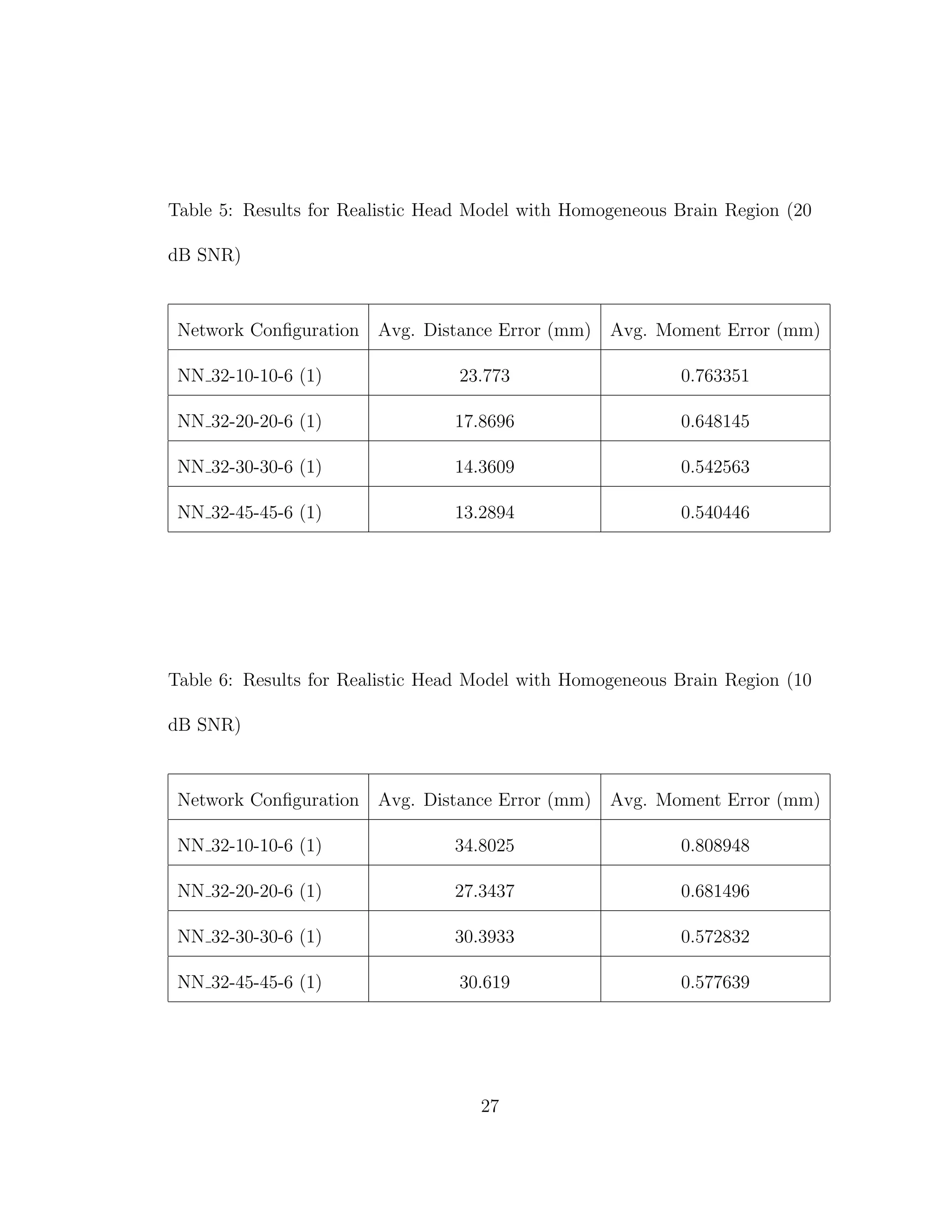
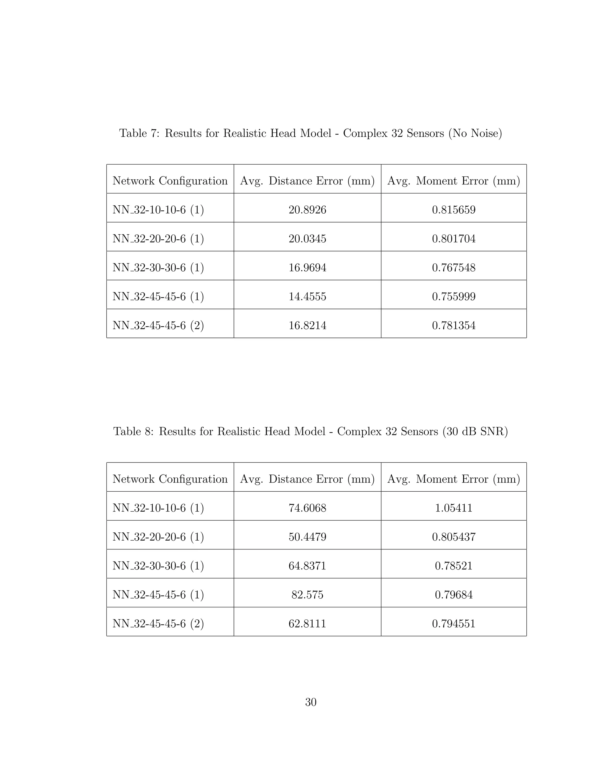
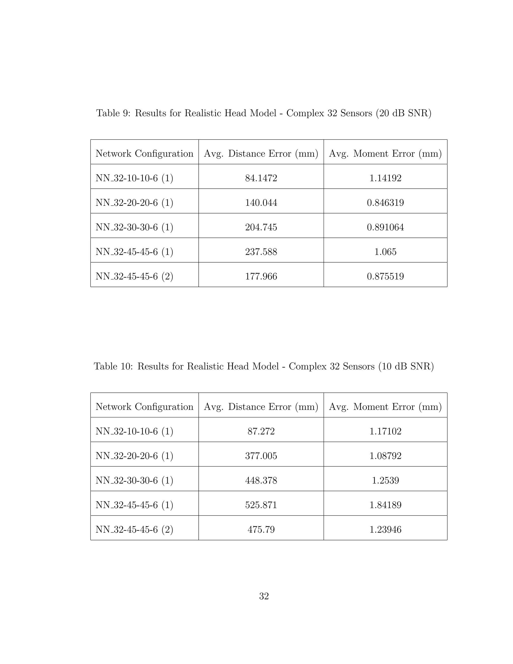
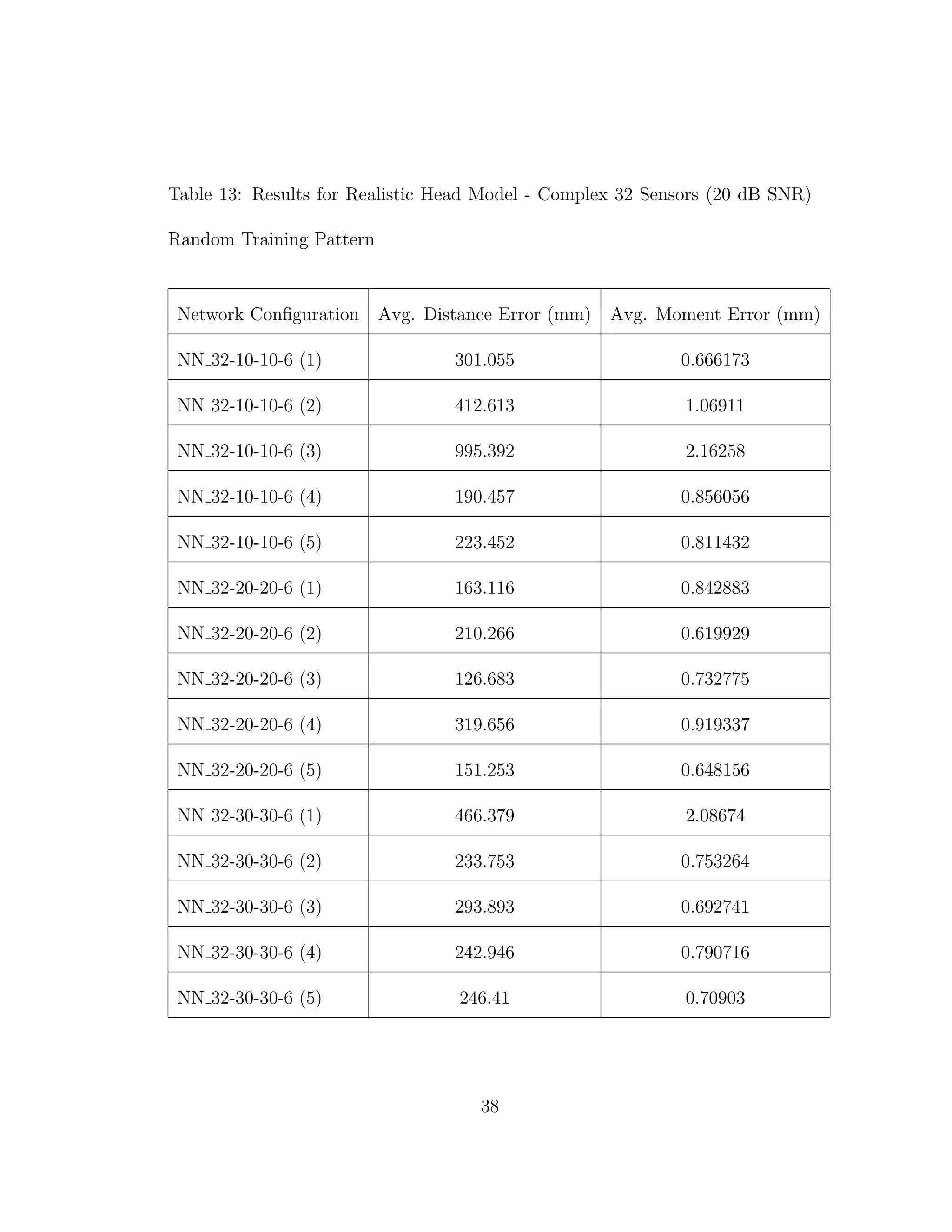
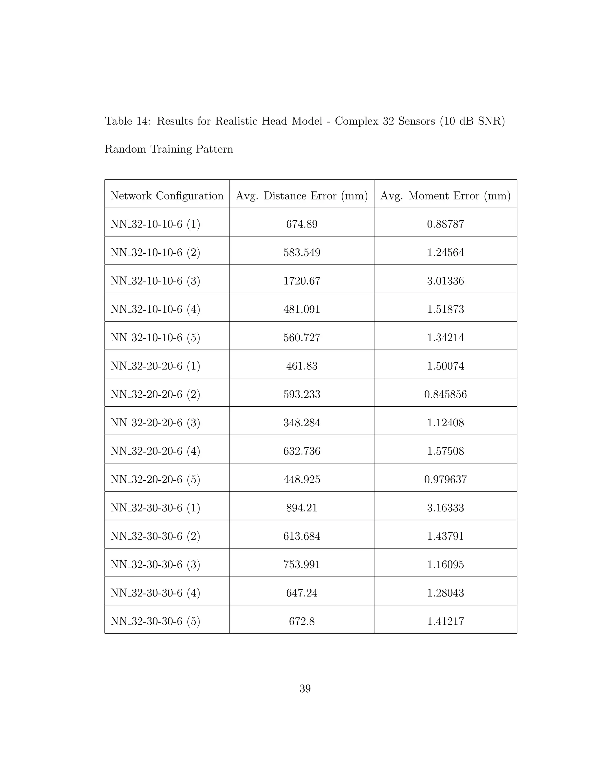
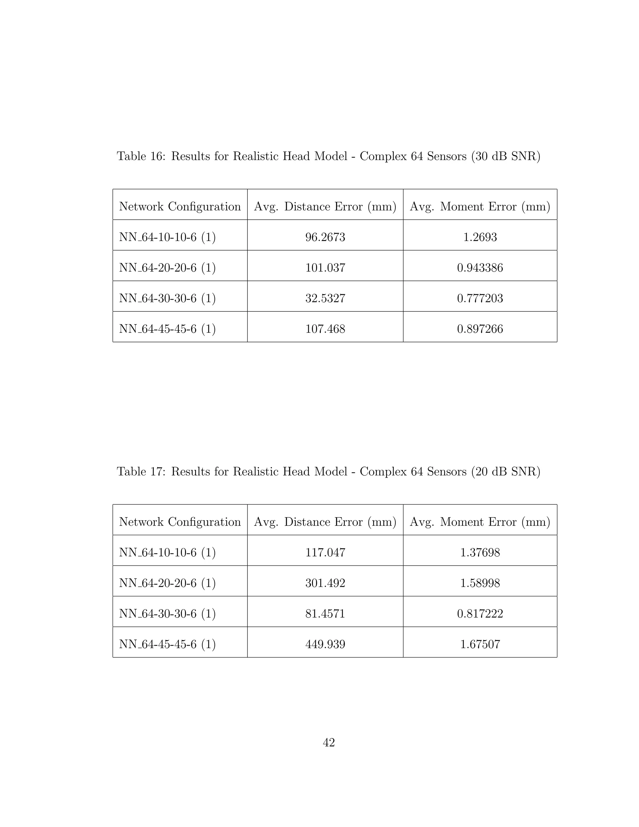
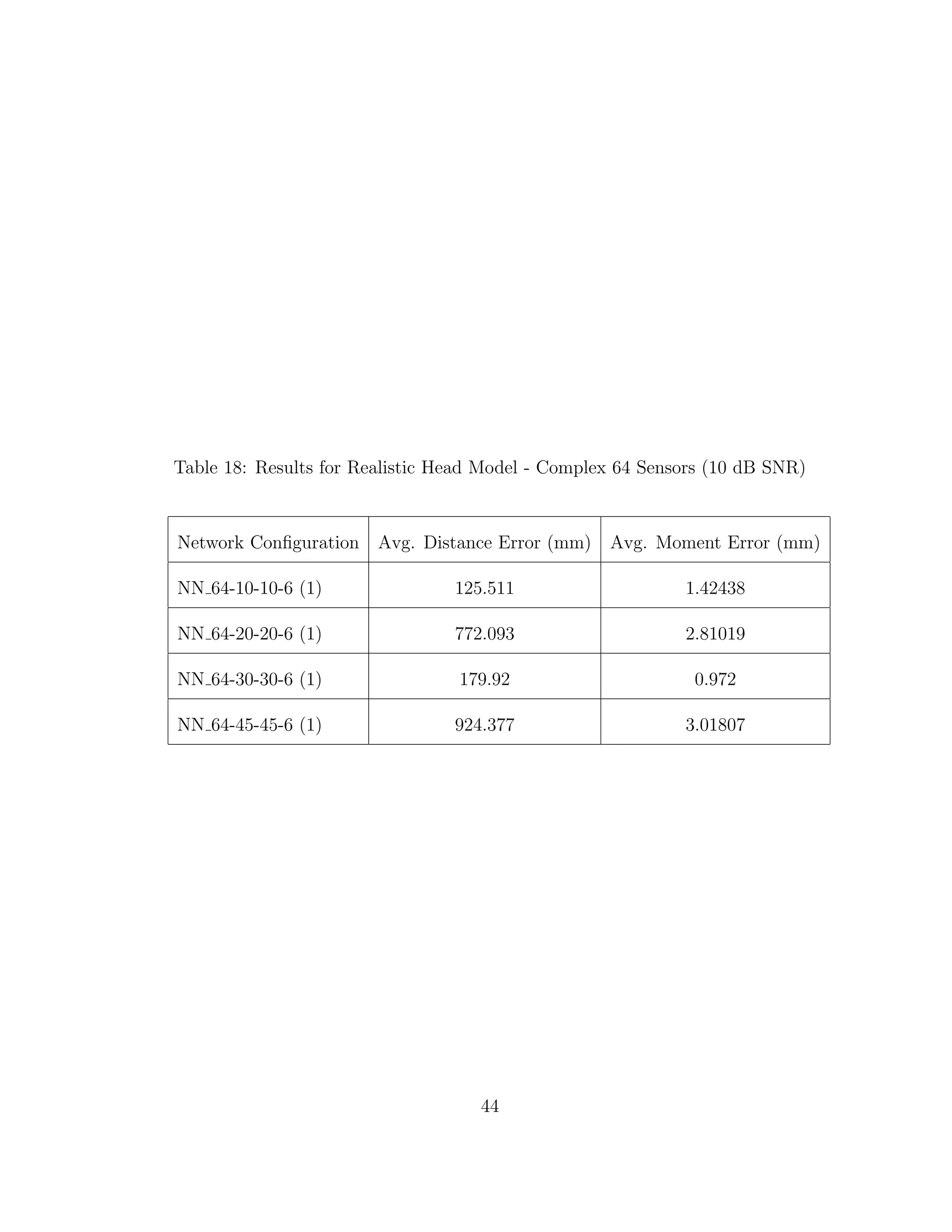
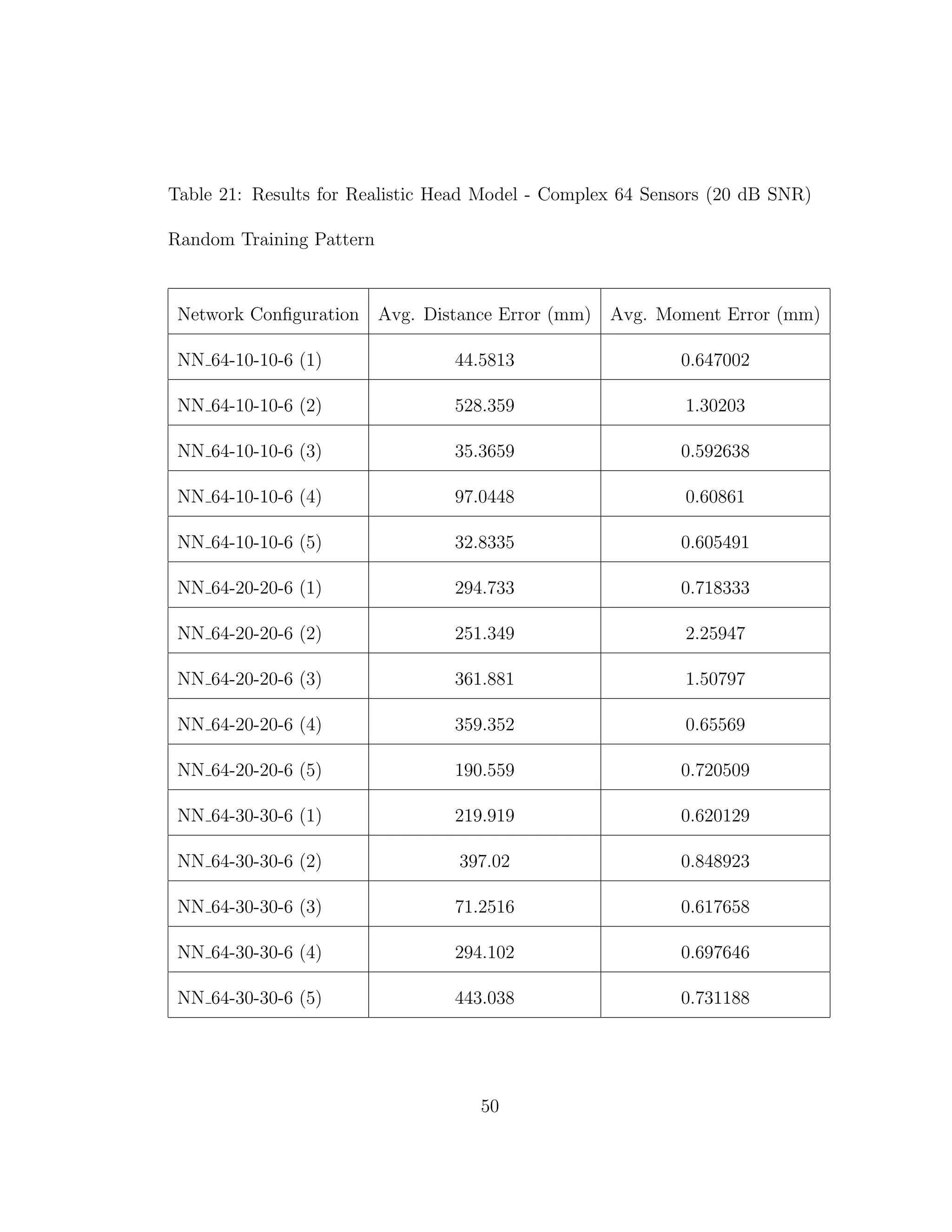
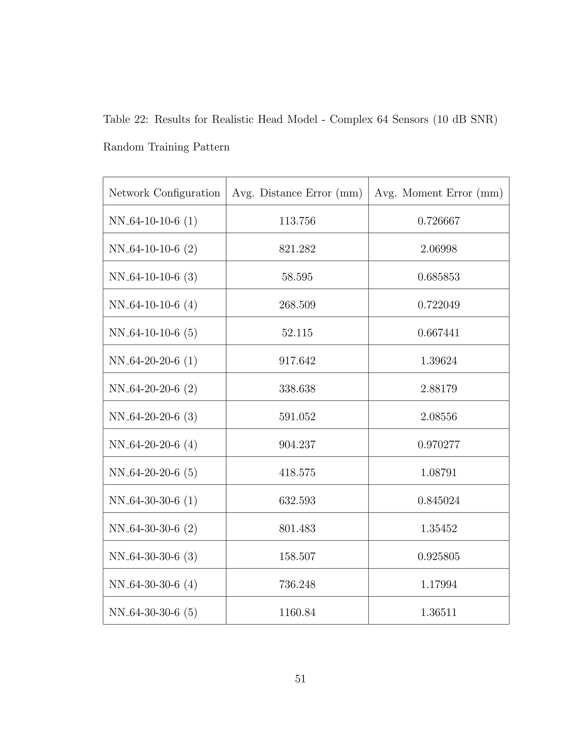
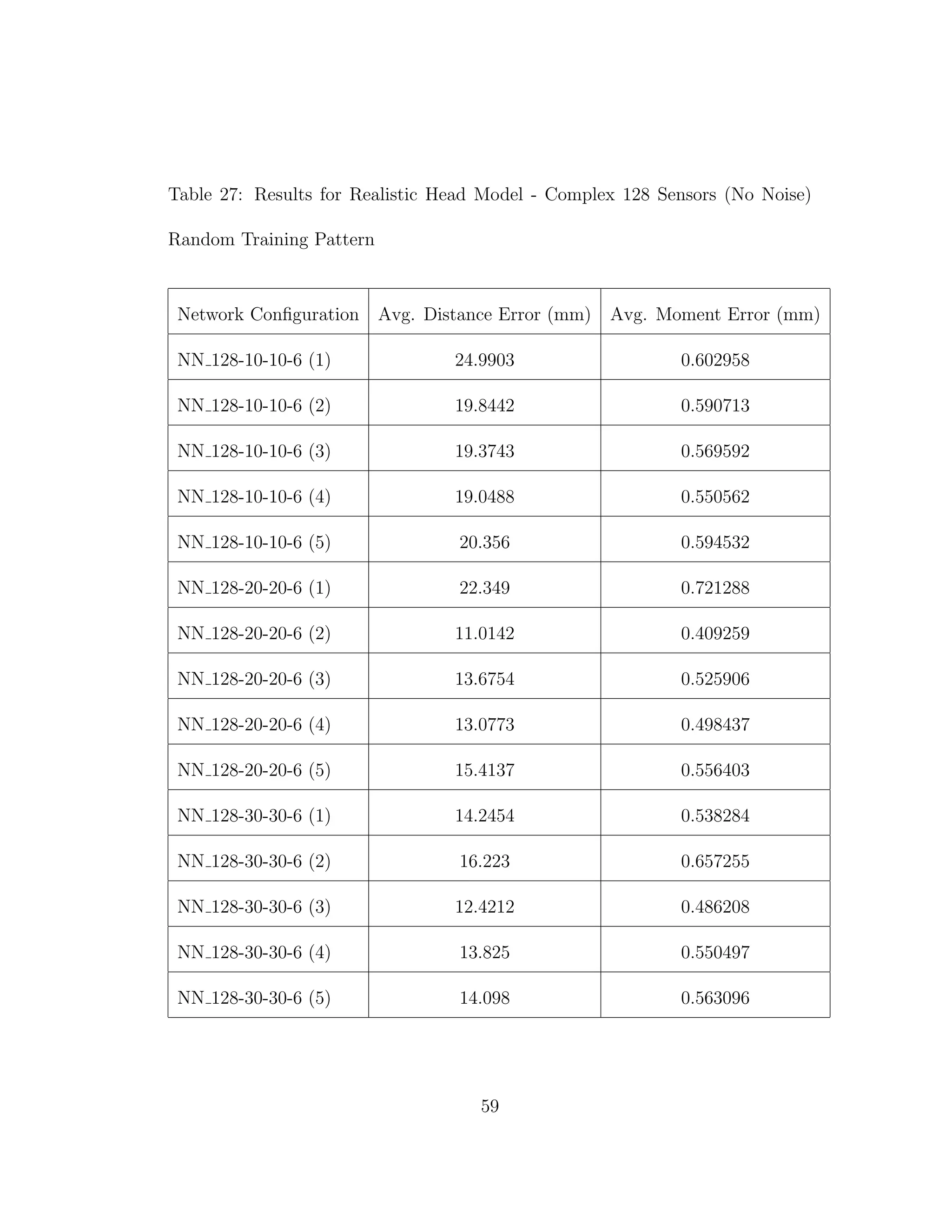
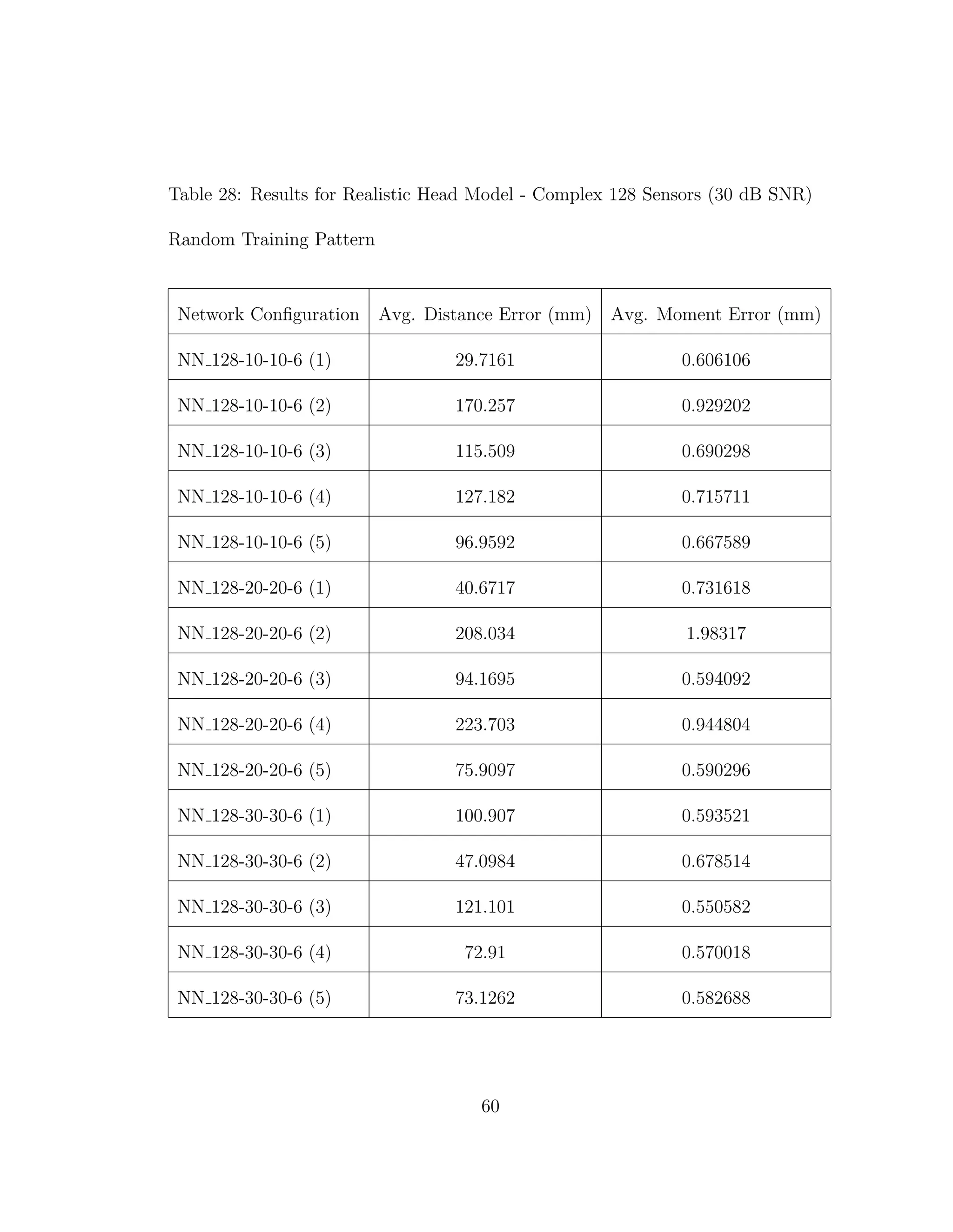
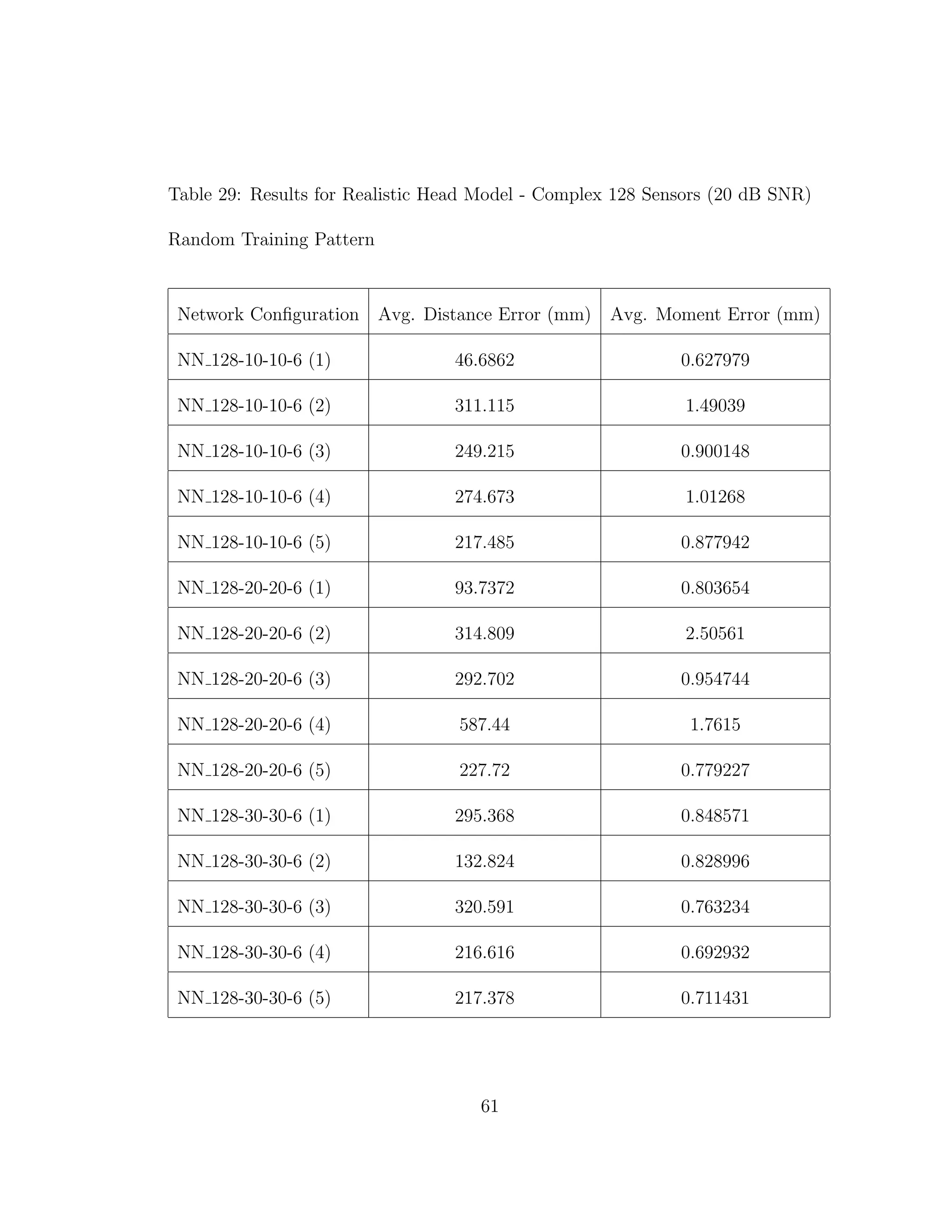
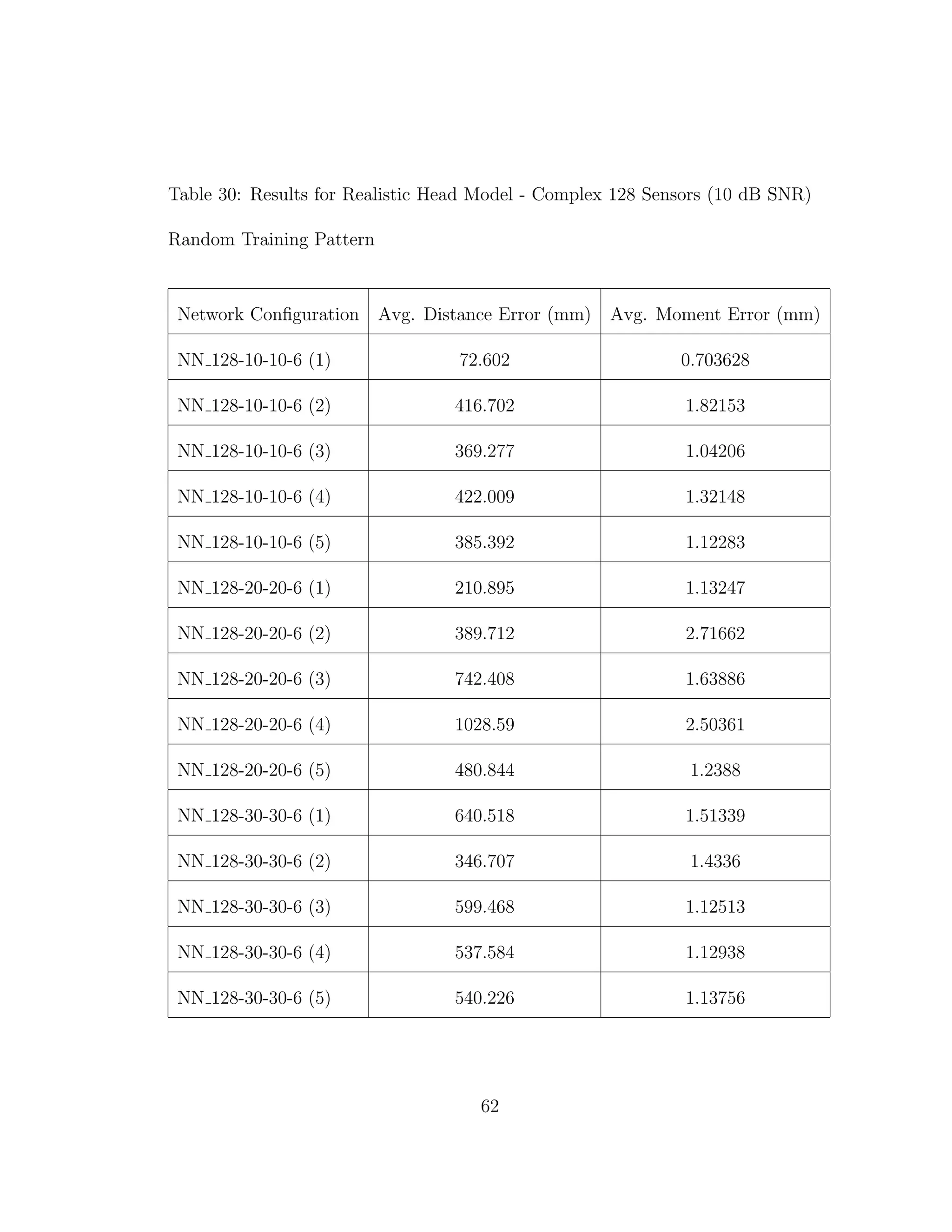
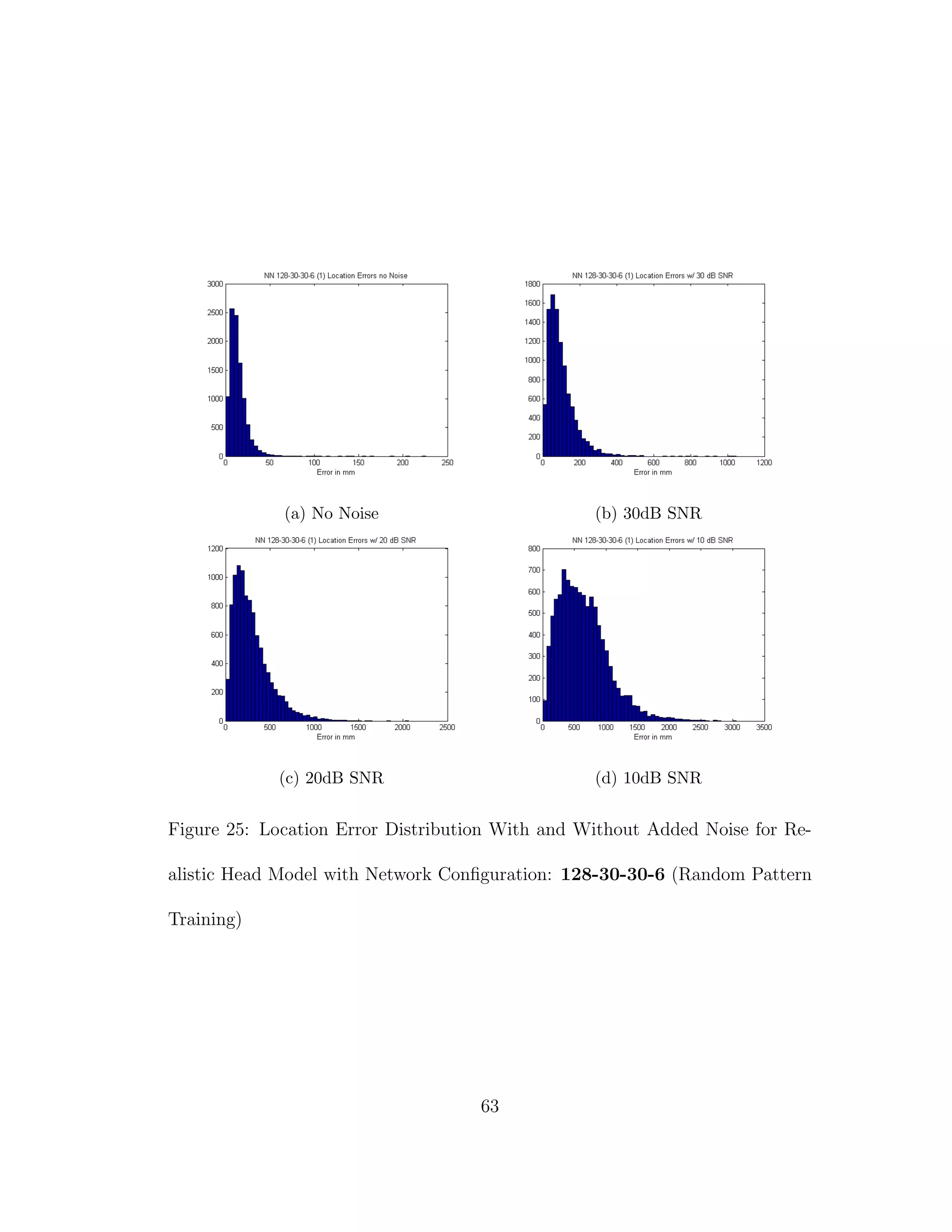
When we compare the results from Tables 3 through 6, the results from our
realistic head model with homogeneous brain area, to Tables 7 through 30, the
results from our more complex realistic head model, we can see a common theme.
For the homogeneous model when we add noise such that the SNR is equal to
30 dB, we only see a jump in average location error of at most 1 mm. This is
completely different in the more complex head model. When we add the same
amount of noise we see jumps in average location error of several centimeters, and
this only gets worse as we add more noise.
Why is this happening? I believe that the reason that a neural network can
source localize a homogeneous head model so well is because of the almost linear
relationship between the dipole and what gets picked up by the sensors on the
64

scalp. If a test dipole is a few millimeters from a training dipole the sensor data
would only be slightly different from the training dipole sensor data. This is what
the network sees when you add noise, data that is slightly different from the real
sensor data. In this case the network will believe that the dipole is in a slightly
different location, therefore the location error is slightly off. As we increase noise
we would expect this to get worse and Tables 3 through 6 show this.
However, if a dipole is a few millimeters from a training dipole in the more
complex realistic head model the sensor data may be significantly different from
the training dipole sensor data. This is because the energy will need to pass
through large patches of white matter before it reaches each sensor on the scalp.
As this power travels through each tissue type it is attenuated at different rates.
Slight differences in sensor data could mean large actual differences in location
between two dipoles. Despite this complexity each of the networks trained for
this model show decent average accuracy with none worse than 2.6 cm and most
less than 2 cm. This can be seen by comparing Tables 7, 11, 15, 19, 23, and
27. When these same networks are presented with the exact same test dipoles,
but with slightly noisy sensor data, 30 dB SNR, the networks become extremely
inaccurate as can be seen in Tables 10, 14, 18, 22, 26, and 30. This tells us that
these networks are extremely sensitive to any abnormality to sensor data, and it
only gets worse as we add more noise.
We can also see this disparity when we look at error histograms from two
65

networks of the same complexity trained with the exact same grid points. One
network is trained for the homogeneous brain model, Figure 13, and one is trained
for the complex head model, Figure 15. Both networks are 32-30-30-6 in configu-
ration. As you can see for the homogeneous brain model as we increase noise error
values get higher, but in all cases error values remain relatively tightly grouped.
For the complex head model error values are initially tightly grouped but a signif-
icant spread forms when we add noise. This trend continues for each other kind
of network trained as can be seen in Figures 17, 19, 21, 23, and 25.
Another point of note is the locations of where the greatest errors are
occurring in each model. To see this I have chosen a layer of voxels on the Z-
plain, around the center of the brain, Z = 178, and tested each point for dipole
location accuracy. These can be seen in Figures 12, 14, 16, 18, 20, 23, and 25.
It is interesting to note that for the homogeneous brain model without noise the
greatest errors occur at the outermost regions, particularly the frontal lobe area,
and areas where training dipoles were scarce, the edges of white matter regions.
For the complex head model without noise the greatest errors occur in all cases
in the frontal lobe area. This does not mean that the complex head model does
not suffer from the same problem with test dipoles at the edge of white matter
regions. In fact for every case the errors in the frontal lobe areas are so bad that
almost all other errors are drowned out. When we restrict the voxels tested to
only be the ones 50 mm from the center of each figure we see the same if not worse
66

error regions than what we see in the homogeneous model.
When we add noise to each case we see something interesting. In the
homogeneous brain model as we increase the noise the greatest errors tend to
occur in the center of the brain. This would be because the signals picked up
from dipoles in the center of the brain would have a much lower power by the
time they reach the sensors, thus making them more susceptible to minor changes
as we would expect. This, however, is not the case with the more complex head
model. In all the cases for the more complex head model the greatest error occurs
in random areas throughout the brain area and gets more random as the noise
increases. This is due to almost all the voxels being very sensitive to noise as
mentioned earlier. And since noise is inherently random we see random error
values everywhere.
67

6 CONCLUSION
Several different configurations were trained for different types of head models:
a 2D universally homogeneous circular head model, a high definition realistic head
model with homogeneous brain region, and a high definition realistic head model
with realistic brain region conductivities.
Each of these networks were subjected to a multitude of tests to determine
average location and moment error with and without noise. The first set of tests
was placing a dipole at every possible grey matter voxel for Z = 178 with its
direction +Z. This was repeated for added noise such that the sensor data had
power of 30 dB, 20 dB, and 10 dB. The next set of tests was placing 10,000 dipoles
at random locations with random directions and determining average location and
moment errors in millimeters. This test was repeated for added noise such that
the sensor data had power of 30 dB, 20 dB, and 10 dB. The error distribution
data for a single network of interest is presented for each model as an example.
In all cases each network is able to reliably source localize a single dipole
with accuracy provide there is absolutely no noise in the signal. Unlike the ho-
mogeneous models, in every case the more complex realistic head model networks
became significantly inaccurate when noise was added to the signal. This is due to
the added complexity that needs to be trained into each of these networks. This
complexity makes these networks far more sensitive to noise.
68

If we can agree that the more complex realistic head model is a better model
of the human head than the realistic head model with a homogeneous brain region,
then it is the recommendation of this author that the network configurations
trained for this project should not be used for clinical use. It may be possible
to achieve better results by segmenting the brain into regions, training neural
networks to source localize in those regions, and training an overall network to
determine what region the dipole resides in. Another option may be to train a
significantly more complex network, however time, memory, and the possibility
of overfitting are all problems to consider. It also may be possible to capture
the complexity of this problem in the increasing popular field of neural-fuzzy
networking.
69

REFERENCES
[1] Abeyratne, Udantha R., Yohsuke Kinouchi, Hideo Oki, Jun Okada, Fumio
Shichijo, and Keizo Matsumoto. ”Artificial Neural Networks for Source Lo-
calization in the Human Brain.” Brain Topography 4.1 (1991): 3-21. Print.
[2] Abeyratne, Uduntha R., G. Zhang, and P. Saratchandran. ”EEG Source Lo-
calization: A Comparative Study of Classical and Neural Network Methods.”
International Journal of Neural Systems 11.4 (2001): 349-59. Print.
[3] Dang, Hung V., and Kwong T. Ng. ”Finite Difference Neuroelectric Modeling
Software.” Journal of Neuroscience Methods 198.2 (2011): 359-63. Print.
[4] Dang, Hung V. ”Performance Analysis of Adaptive EEG Beamformers.” Diss.
New Mexico State University, 2007. Print.
[5] Hagan, Martin T., Howard B. Demuth, and Mark H. Beale. Neural Network
Design. Boulder, CO: Distributed by Campus Pub. Service, University of
Colorado Bookstore, 2002. Print.
[6] Jenkinson, M., CF Beckmann, TE Behrens, MW Woolrich, and SM Smith.
”FSL.” NeuroImage 62 (2012): 782-90. Print.
[7] Kamijo, Ken’ichi, Tomoharu Kiyuna, Yoko Takaki, Akihisa Kenmochi, Tet-
suji Tanigawa, and Toshimasa Yamazaki. ”Integrated Approach of an Artifi-
cial Neural Network and Numerical Analysis to Multiple Equivalent Current
Dipole Source Localization.” Frontiers of Medical & Biological Engineering
10.4 (2001): 285-301. Print.
[8] Lau, Clifford. Neural Networks: Theoretical Foundations and Analysis. New
York: IEEE, 1992. Print.
[9] Steinberg, Ben Zion, Mark J. Beran, Steven H. Chin, and James H. Howard,
Jr. ”A Neural Network Approach to Source Localization.” The Journal of the
Acoustical Society of America 90.4 (1991): 2081-090. Print.
[10] Van Hoey, Gert, Jeremy De Clercq, Bart Vanrumste, Rik Van De Walle,
Ignace Lemahieu, Michel D’Have, and Paul Boon. ”EEG Dipole Source Lo-
calization Using Artificial Neural Networks.” Physics in Medicine & Biology
45.4 (2000): 997-1011. IOPscience. Web. 22 May 2013.
[11] Vemuri, V. Rao. Artificial Neural Networks: Concepts and Control Applica-
tions. Los Alamitos, CA: IEEE Computer Society, 1992. Print.
70

[12] Yuasa, Motohiro, Qinyu Zhang, Hirofumi Nagashino, and Yohsuke Kinouchi.
”EEG Source Localization for Two Dipoles by Neural Networks.” Proceedings
of the 20th Annual International Conference of the IEEE Engineering in
Medicine and Biology Society 20.4 (1998): 2190-192. Print.
[13] Yushkevich, Paul A., Joseph Piven, Heather Cody Hazlett, Rachel Gimpel
Smith, Sean Ho, James C. Gee, and Guido Gerig. ”User-guided 3D Active
Contour Segmentation of Anatomical Structures: Signiﬁcantly Improved Ef-
ﬁciency and Reliability.” NeuroImage 31.3 (2006): 1116-128. Print.
[14] Zhang, Q., X. Bai, M. Akutagawa, H. Nagashino, Y. Kinouchi, F. Shichijo,
S. Nagahiro, and L. Ding. ”A Method for Two EEG Sources Localization
by Combining BP Neural Networks with Nonlinear Least Square Method.”
Control, Automation, Robotics and Vision, 2002. ICARCV 2002. 7th Inter-
national Conference 1 (2002): 536-41. Print.
[15] Zhang, Qinyu, Motohiro Yuasa, Hirofumi Nagashino, and Yohsuke Kinouchi.
”Single Dipole Source Localization From Conventional EEG Using BP Neural
Networks.” Engineering in Medicine and Biology Society, 1998. Proceedings
of the 20th Annual International Conference of the IEEE 4 (1998): 2163-166.
Print.
71

Berard - Thesis

Recommended

Recommended

More Related Content

What's hot

What's hot (20)

Viewers also liked

Viewers also liked (16)

Similar to Berard - Thesis

Similar to Berard - Thesis (20)

Berard - Thesis