Download to read offline


![Introduction
These days, optical networks can be found anywhere from the access level to the
very core of the Internet. But it is in the transmission of large amounts of infor-
mation over long distances that they provide indisputable advantages over other
transport technologies. The following dissertation focuses on such long-distance
optical networks, also referred to as backbone, long-haul or core networks [102].
Most current backbone optical networks are built on two main cornerstones.
First, they are circuit-switching networks. That is to say, user information is sent
between a pair of source-destination nodes as a continuous constant-rate bitstream
that follows the same route or path across the network. Here, a node represents a
point in the network where information can be transmitted, received or forwarded.
Second, their data plane is not all-optical. In other words, the bitstream containing
user information is sent optically through the links of the network, but is converted
to electronic signals at its nodes.
This scenario is not static or permanent. Optical networks are constantly
evolving in an attempt to meet the ever-increasing demand for bandwidth created
by the expansion of the Internet. This expansion has been one of the main catalysts
behind the unprecedented growth of optical networks in the past several years.
However, it has also created a demand for new dynamic and upgradeable optical
networks.
The need for dynamic optical networks is conrmed by many empirical studies
reporting that Internet trac is highly variable and bursty (see for instance [31,
55, 96, 42]). An ecient and natural way of coping with such variable trac is
to use packet-switching optical networks [115]. In such networks, user information](https://image.slidesharecdn.com/3f7f65b2-eeec-4afd-a395-b25a5ff55a20-160530113535/85/Modeling_Future_All_Optical_Networks_without_Buff-15-320.jpg)
![ii
is sent between a pair of source-destination nodes as a series of packets that may
follow dierent routes, where a packet is a nite sequence of bits. Thus, one of the
major trends in the design of future optical networks is to move from the current
circuit-switching to the packet-switching paradigm [138, 83].
The need for upgradeable optical networks arises from the continuously-in-
creasing demand for bandwidth prompted by the expansion of the Internet. An
ecient way of designing an upgradeable network is to make it all-optical - that
is, to use exclusively optical components for the transmission of user information
across the network. Indeed, it is relatively simple to upgrade the data rate in all-
optical networks by adding extra transmission channels [16]. Moreover, all-optical
networks have at least two additional advantages. First, they can potentially
reduce costs by saving on expensive electronics and opto-electro-optic (O/E/O)
converters, and by reducing power consumption. Second, they can eliminate the so-
called electronic bottleneck. This bottleneck is currently one of the major factors
limiting capacity in an optical network. It is a result of the low processing speed of
the electronic equipment at the nodes compared to the high transmission capacity
at the optical links. All these advantages make all-optical networking another
major trend in the design of future optical networks [136, 138, 83, 134, 121].
The two trends mentioned above give rise to the concept of a pure packet-
oriented all-optical network, called an Optical Packet Switching (OPS) network in
the literature [138, 83]. The main objective in the design of an OPS network is to
maximize its performance. Secondary objectives are the cost and feasibility of the
all-optical hardware components needed.
The term performance is somewhat ambiguous. It can refer to the eciency
with which bits are physically represented, transferred and received in a network.
Typical performance parameters in this case are the bit error rate (BER) or the
signal-to-noise ratio (SNR) [4]. Performance can also refer to the eciency with
which packets are transferred through the network by the network protocols. Net-
work protocols can delay and sometimes cause the loss of packets. The main
performance parameters in this case are the average packet delay and the packet
blocking probability, which basically refers to the probability that a packet will
be lost in the network. In this dissertation, we are interested in the study of a
packet-switching all-optical network at the packet level of abstraction (i.e., at the
OSI network layer). Thus, the term performance will hereinafter be used in order
to refer to the average packet delay and the packet blocking probability.
In order to maximize the performance of an OPS network, it is customary to
include the following three requirements in its denition [136, 138, 83]. First, not
only the data plane, but also the control plane must be all-optical. That is to
say, signaling information used to manage network bandwidth must be processed
optically. This allows the control plane to prot from the above-mentioned benets](https://image.slidesharecdn.com/3f7f65b2-eeec-4afd-a395-b25a5ff55a20-160530113535/85/Modeling_Future_All_Optical_Networks_without_Buff-16-320.jpg)
![iii
of an all-optical implementation. Second, incoming electronic packets must be sent
on the y (i.e., as they arrive) through the optical domain. This minimizes packet
delay at the ingress nodes in the network. Third, buering must be available at the
optical domain, permitting the reduction of the blocking probability and thereby
increasing network throughput.
The downside of these three requirements is that they notably increase the
complexity associated with the implementation of an OPS network [83]. More
specically, the rst requirement implies the use of extensive signal processing ca-
pabilities at the optical domain, a technology that is not yet mature enough [19].
The second requirement implies that optical packets have the same size as incom-
ing Internet (IP) packets. This sets the operating times of the optical components
in the OPS network (e.g., the switching times) to the ns range [28], represent-
ing a considerable challenge for current technology. The third requirement also
represents a problem, because there is no optical equivalent to the random access
memory (RAM) used to build the buers in electronic packet-switching networks.
The best option available are ber delay lines (FDLs), which are more expensive
and dicult to control than RAMs [44], and increase signal degradation at the
optical domain due to physical system impairments [116].
The fact that OPS networks are so dicult to implement creates room for
alternative networking solutions, where lower performance is accepted in exchange
for a less expensive and complex hardware implementation. One such alternative
solution is Optical Burst Switching (OBS).
The denition of an OBS network strategically avoids the use of the three
requirements presented above, while still remaining faithful to the basic principles
of a packet-switching all-optical network [134, 135]. First, the control plane is
implemented electronically (although the data plane is still all-optical). Second,
incoming electronic packets are buered at the ingress nodes in the network in
order to form large groups of packets called bursts, which are then transferred
through the optical domain. This relaxes the operating time requirements from
the ns to the µs range [67]. Third, as buering is not available at the optical
domain, the use of FDLs is avoided. These characteristics will most probably
enable OBS networks to be implemented earlier and at a lower cost than OPS
networks [121].
Research on OBS networks has been quite extensive in the last decade and
focuses mainly on two questions. The rst question is whether OBS networks can
be deployed soon and in a cost-ecient manner. The second question is whether
OBS networks can provide a clear advantage in terms of performance compared
to current optical network architectures.
This thesis focuses on the second question formulated above. Our main objec-
tive is to provide the research community with a tractable and reliable analytical](https://image.slidesharecdn.com/3f7f65b2-eeec-4afd-a395-b25a5ff55a20-160530113535/85/Modeling_Future_All_Optical_Networks_without_Buff-17-320.jpg)
![iv
network model that can be used in order to assess the performance in OBS net-
works in terms of the burst blocking probability. By tractable we mean a model
from which the blocking probability can be computed within a reasonable time
using a reasonable amount of computational resources. By reliable we mean a
model that includes enough functional and structural details from the original
OBS network in order to be realistic and accurate. The use of our analytical net-
work model to actually evaluate the viability of OBS networks is out of the scope
of this dissertation.
It turns out that the model developed for OBS networks in this thesis can
also be used in order to model OPS networks without buering capabilities (i.e.,
without FDLs), also denoted as buerless OPS networks. These networks are
of great practical importance, since their study can help to decide whether it is
necessary or not to invest resources in the development and use of FDLs for OPS
networks [82, 81].
The blocking probability is the performance parameter of interest in our net-
work model, since neither OBS nor buerless OPS networks have FDLs to reduce
blocking at the core nodes. It has also been the preferred performance parameter
studied in the literature on OPS/OBS networks [167, 99, 167, 66].
The study of other performance parameters falls out of the scope of this doc-
ument. Such is the case of the results published in [40]. In that paper, we present
a new framework to study the problem of planning an OBS network from scratch.
The objective is to ensure that ows in the network meet previously given QoS
(Quality of Service) requirements in the form of maximum average packet delay
and blocking probability.
In this thesis, we develop the analytical network model of a buerless OPS/OBS
network in three steps that we call the Network step, the Trac step and the
Modeling step. In the Network step, the objective is to study the optical network
in detail and to decide which aspects of its functionality and structure should be
included in the network model. In the Trac step, the goal is to study network
trac in detail and to decide which statistical properties should be included in the
network model. In both steps, the main criterium used to select the information
to be included in the network model is an often dicult compromise between its
resulting reliability and mathematical tractability. In the Modeling step, the goal
is to produce the analytical network model based on the modeling considerations
collected in the previous steps, together with the corresponding algorithm for the
computation of the blocking probability.
The three steps mentioned above serve as the backbone for structuring this
work and are reected in the three parts into which this thesis is divided. We
proceed now to explain each part.](https://image.slidesharecdn.com/3f7f65b2-eeec-4afd-a395-b25a5ff55a20-160530113535/85/Modeling_Future_All_Optical_Networks_without_Buff-18-320.jpg)
![v
Part I: Networks. This part presents functional and structural details con-
cerning the buerless OPS/OBS network to be modeled here. As stated before,
the main goal is to identify the most important features of a buerless OPS/OBS
network in order to take them into account in the network model developed in
Part III of this thesis. This, and the associated literature survey are the main
contributions from this part.
OPS and OBS networks constitute extremely active research elds. It is there-
fore not surprising that many variants of these networks have been presented and
studied in the literature. Designing a model for a particular variant has the dis-
advantage of reducing its use to just that variant. Designing a model for each one
of the dierent variants constitutes a lengthy task beyond the scope of any single
dissertation. In this work, we have opted for a third possibility and designed a
model for a basic or standard version of an OBS network, the origin of all other
variants. This standard version corresponds to the concept of OBS networking, as
originally introduced by Qiao and Yoo in [134, 135]. The resulting model is also
valid for a standard OPS network as presented in [108], but without FDLs at the
core nodes.
Part I focuses on the description of the above-mentioned standard versions of
a buerless OPS/OBS network. This document does not include the study of any
variants. Such studies can be found in [41] and [131], contributions from which
will be briey summarized here.
OBS core nodes use algorithms called reservation mechanisms in order to re-
serve a portion of bandwidth on a link for the transmission of a burst upon the
arrival of its associated header packet. In [41] we present a new reservation mech-
anism for OBS networks. We show analytically that it performs better than the
best state-of-the-art reservation mechanism in terms of burst blocking probability,
and that it allows for a less complex and cheaper network implementation.
Many authors predict performance problems if an OBS network uses the TCP
(Transmission Control Protocol) as a transport protocol [72, 77, 168, 24, 43].
In [131] we put these results into perspective by reporting that when the num-
ber of TCP end users is high (above 100) and a realistic version such as TCP Reno
is used, performance is not severely aected by the use of TCP in OBS networks.
Part I is divided into two chapters. Chapter 1 provides an introduction to OPS
and OBS networks as a particular type of all-optical network. The main focus is
on a functional or procedural description of their four basic elements: ingress edge
nodes, transmission links, core nodes and egress edge nodes. Essentially, we limit
ourselves to the description of what these elements do in order to transfer user
information through the network, and intentionally skip the details concerning
their structure and hardware implementation. At the end of the chapter, we](https://image.slidesharecdn.com/3f7f65b2-eeec-4afd-a395-b25a5ff55a20-160530113535/85/Modeling_Future_All_Optical_Networks_without_Buff-19-320.jpg)
![vi
identify the most relevant functional features of buerless OPS/OBS networks in
order to take them into account in the network model developed in Part III.
In Chapter 2 we study the hardware implementation of an OBS network. The
main goal is to identify the most important structural features to be considered in
the analytical model in Part III. The idea here is to describe how the basic elements
in an OBS network can be modeled, based on their particular hardware implemen-
tation. A secondary goal is to provide the reader with information concerning the
state-of-the-art techniques for implementing an OBS network.
The hardware implementation of our standard buerless OPS network from [108]
is very similar to that of our standard OBS network from [134, 135]. There are basi-
cally only two main dierences. First, hardware operating times for OPS networks
are at least three orders of magnitude below those for OBS networks [67, 28]. Sec-
ond, OPS networks require the development of new tailor-made optical hardware
for the implementation of the control plane in the optical domain. These dier-
ences play a crucial role in the commercial potential of each one of the networking
solutions. However, from the structural point of view, the hardware implementa-
tion of the data plane in these networks is the same in both cases [16]. For this
reason, structural modeling features from the data plane identied in this chapter
are assumed to be valid for buerless OPS networks as well.
Part II: Trac. This part presents a study of the trac inside a buerless
OPS/OBS network. The main goal is to identify which statistical properties of
this trac should be taken into account in the network model developed in Part
III.
Buerless OPS/OBS networks are not yet commercially available, and thus it
is not possible to directly measure the statistical properties of their trac. In
Part II we overcome this problem by means of a two-step approach. In Chapter 3
we study the statistical properties of the trac that is most likely to arrive at a
buerless OPS/OBS network. In Chapter 4 we deduce from the results of Chapter
3 the statistical properties of trac entering the optical domain in a buerless
OPS/OBS network.
Buerless OPS/OBS networks constitute backbone network solutions and as
such are expected to receive highly-aggregated Internet (or IP) trac at their
ingress nodes [74, 138, 26, 133]. That trac exhibits a high throughput result-
ing from the aggregation of many individual IP ows. Thus, it is possible to
study current highly-aggregated trac from the Internet backbone and assume
that similar trac will arrive at future buerless OPS/OBS networks. Accordingly,
our main goal in Chapter 3 is to gain insight on the statistical nature of highly-](https://image.slidesharecdn.com/3f7f65b2-eeec-4afd-a395-b25a5ff55a20-160530113535/85/Modeling_Future_All_Optical_Networks_without_Buff-20-320.jpg)
![vii
aggregated IP trac as representative of the trac entering a typical buerless
OPS/OBS network. Previous studies report contradictory results on this matter.
On the one hand, some authors have reported the existence of long-memory or
long-range dependent (LRD) properties in low-aggregated [107, 35] as well as in
highly-aggregated IP trac [126]. On the other hand, papers such as [22, 23, 96]
acknowledge the existence of LRD in low-aggregated IP trac, but report that
as the level of aggregation increases, LRD disappears and trac progressively re-
sembles a Poisson process. Perhaps inspired by this conclusion, the majority of
publications in the eld of backbone optical networks use models with Poisson
trac (see for instance [80, 46, 141]).
Theoretically, in order to settle the debate on the statistical nature of highly-
aggregated IP trac, one could simply perform a statistical analysis of network
trac in a high-capacity optical backbone link. In practice, two main diculties
arise when trying to accomplish such a task. First, due to condentiality issues, it
is dicult for the research community to access such information, owned in most
cases by private network operators. Second, the ecient measurement of trac at
Gbps speeds is a very challenging technical task. Hardware limitations often reduce
the precision of the packet time-stamps to µs, as in [96]. Software limitations have
an impact on the amount of data that can be analyzed and therefore often reduce
the signicance of the results obtained.
Our contribution to this debate is a detailed statistical analysis of a set of two
trac traces provided by the Universitat Politècnica de Catalunya (UPC) within
the framework of the European-funded research projects NOBEL I and NOBEL
II [132]. These traces contain an unprecedent amount of accurate data taken
from a highly-aggregated transmission link. More specically, each trace contains
approximately 800 million packet arrival time and packet size measurements from
a 2-Gbps link, where packet arrival times are measured with ns-precision.
Our main result is a rejection of the Poisson hypothesis and strong evidence
suggesting the presence of LRD in all the traces analyzed. This result is important,
since it is widely known that LRD has a signicant negative impact on network
performance, measured in terms of such parameters as the buer dynamics and
blocking probability [126, 63].
We conducted additional studies in order to determine scaling properties in the
trac beyond LRD. In particular, in [42, 21] we studied the multifractal proper-
ties of trac (see [55]) by means of the Multiscale Diagram presented in [2, 164].
However, we do not include these results in the dissertation for two reasons. First,
in [164] the authors express their reservations about the eectiveness of the Multi-
scale Diagram and other standard tests for detecting the presence of multifractal
behavior. Second, even if it could be eectively detected, it is not clear that
multifractal trac has a substantial impact on network performance [9].](https://image.slidesharecdn.com/3f7f65b2-eeec-4afd-a395-b25a5ff55a20-160530113535/85/Modeling_Future_All_Optical_Networks_without_Buff-21-320.jpg)
![viii
In Chapter 4, we assume the existence of LRD IP trac arriving at the ingress
edge nodes in an OPS/OBS network (in line with the evidence reported in Chapter
3) and study if and how LRD is transferred to the departure trac from these
nodes. That is, we study whether LRD is injected into the optical domain in
OPS/OBS networks. As mentioned before, this question is relevant because of the
impact that LRD trac has on network performance.
In OPS networks, the answer to this question is immediately evident. In these
networks, incoming IP packets are sent directly through the optical domain as
they arrive at the ingress edge nodes. An immediate implication of this is that
the statistical properties of incoming IP trac are not modied by the ingress
edge nodes in the OPS network. Thus, we conclude that LRD should be taken
into account in the network model of Part III of this thesis, whenever it is used to
model a buerless OPS network.
In the case of OBS networks the situation is more complex. Indeed, the char-
acteristics of trac entering the optical domain in an OBS network are generally
dierent from those of the incoming electronic trac, due to the fact that incom-
ing IP packets are buered at the ingress nodes to form bursts. In OBS networks,
buering is controlled by an algorithm called the aggregation strategy (AS). The
AS basically decides how many incoming packets should be buered in order to
create a burst. Thus, the question of whether the burst trac entering the OBS
network inherits the LRD from the electronic input trac is dependent on the
choice of the AS.
There are four main ASs presented in the literature: the Timeout, Buer Limit,
Packet Count and Mixed ASs [179, 69, 39, 172].
The impact of the Timeout AS on the degree of LRD of the burst trac entering
an OBS network has been studied in [69, 86, 179, 8, 78, 153]. The methodology
followed in [69, 8, 78, 153] is the use of simulation techniques together with dierent
Hurst parameter estimators to measure the degree of LRD. In [86, 179], several
analytical approximations and asymptotic bounds are obtained. Except for some
discrepancies (see [179, 78]), the general conclusion is that LRD does not seem to
be substantially reduced by the buering that takes place at ingress OBS nodes
using the Timeout AS.
There do not appear to be any equivalent studies in the literature for the other
three ASs, and thus the state-of-the-art picture of trac entering an OBS network
is incomplete. In Chapter 4, we complete this picture by extending the study to
the Packet Count, Buer Limit and Mixed ASs. Our methodology includes both
analytical and simulation studies. From the theoretical point of view, our main
contribution is a new analytical approach based on the discrete wavelet transform
(DWT) to study the presence of LRD in the burst trac entering an OBS network.
In the case of the Packet Count AS, our approach provides exact results, which](https://image.slidesharecdn.com/3f7f65b2-eeec-4afd-a395-b25a5ff55a20-160530113535/85/Modeling_Future_All_Optical_Networks_without_Buff-22-320.jpg)
![ix
contrasts with the fact that until now only approximate results had been obtained
for the Timeout AS in [86, 179]. In the case of the Buer Limit AS, our approach
provides approximate results.
The analytical and simulative results from this chapter all suggest that LRD
is neither eliminated nor modied (i.e., the Hurst parameter does not change)
by the main four ASs in an OBS network. Therefore, our main conclusion from
Part II is that LRD should be taken into account when modeling burst trac
entering a buerless OPS/OBS network. This conclusion questions the common
practice of using the Poisson trac assumption in models of backbone optical
networks [80, 46, 141].
Part III: Modeling. This part presents the main results of this dissertation:
a new model of a buerless OPS/OBS network together with an algorithm for
the computation of the blocking probability at any point in the network. As was
explained earlier in this introduction, our goal is to obtain a model that is both
reliable and tractable. In order for the model to be reliable, it should incorporate
the most important features from Part I concerning the functionality and structure
of a typical buerless OPS/OBS network, as well as those from Part II concerning
the statistical properties of its trac. In order for the model to be tractable,
the algorithm for computing the blocking probability should converge within a
reasonable time using a reasonable amount of computational resources.
Chapter 5 presents a preliminary model of a buerless OPS/OBS network and
shows how to compute the blocking probability at any point in it. The preliminary
model includes all the modeling features from Part I, but does not take into account
the result from Part II concerning the LRD nature of burst trac entering a
buerless OPS/OBS network. Instead, the main assumption in this chapter is
that packets/bursts enter the optical domain (i.e., leave the ingress edge nodes)
according to a Poisson process.
Although the assumption above goes against our ndings in Part II the resulting
model is by no means immediately evident, due to the fact that buerless packet-
switching networks exhibit complex behavior. In such networks, packets from a
source interact on each link with packets from other sources routed through that
link. The physical origin of this interaction is the loss of packets (i.e., blocking)
caused by the fact that packets from dierent sources must share a nite number
of transmission channels on each link. As a result of packet loss, the characteristics
of a trac source change whenever it is routed on a link together with other trac.
Therefore, a complete description of the trac on each link in the network requires
full knowledge of the changes accumulated as packets from each source share links
along their path with packets from other sources.](https://image.slidesharecdn.com/3f7f65b2-eeec-4afd-a395-b25a5ff55a20-160530113535/85/Modeling_Future_All_Optical_Networks_without_Buff-23-320.jpg)
![x
Previous models of buerless packet-switching networks, such as [46, 45, 173,
5, 141, 167, 163, 159], do not provide a complete description (in the sense given
above) of the trac on each link in the network for two reasons. First, in these
models, packets are assumed to arrive at each node in the network according to the
same type of process (e.g., a Poisson process). That is to say, the packet arrival
process is re-sampled at each node in the network. Second, in these models, packet
transmission times (and therefore packet sizes) are assumed to be re-sampled at
each node in the network (e.g., from an exponential distribution). Re-sampling
of these two stochastic processes (sometimes referred to as link blocking indepen-
dence [163]) inevitably implies the loss of information concerning the blocking
events of packets along the routes in the network, which makes the description of
trac incomplete.
The most outstanding feature of our model is the fact that, to our knowledge,
it incorporates for the rst time a complete description (in the sense given above)
of the trac on each link in the network.
Our model belongs to the class of reversible Markov process models described
in [144], and it is related to well-known stochastic network models used in circuit-
switching networking scenarios, such as [129, 29, 104, 103]. The main dierence
is that in these circuit-switching models there is just one so-called multivariate
birth-death (BD) process to describe trac in the whole network, while in our
case we have a dierent one to describe the trac on each link in the network.
Regarding the computation of the blocking probability in our model, we show
in this chapter that it all comes down to the computation of the well-known par-
tition function [144, 129, 29, 104, 103]. This function has been studied over the
last two decades within the framework of many models of circuit-switching net-
works. In [109] it was demonstrated that its exact computation constitutes a P-
complete problem, where the class P-complete is a subset of the NP-complete
problems. According to current notions in complexity theory, it is widely believed
that no polynomial-time algorithm exists to solve any problem that belongs to the
NP-complete class [64]. This suggests serious scalability problems aecting the
computation of the blocking probability in our model as the size of the network
grows. In the case of the circuit-switching models presented above, such scalability
problems have been solved with the use of Monte Carlo simulation techniques [62].
These techniques provide an estimation of the value of the partition function and
thus of the blocking probability. Since their complexity does not depend on the
size of the network, they do not present any scalability issues. In Chapter 5 we use
a numerical example to demonstrate that the use of Monte Carlo simulation tech-
niques from [104, 103] leads to an accurate estimation of the blocking probability
at dierent points in our network. This allows us to conclude that our model is
tractable, since the blocking probability can be accurately estimated, even in large](https://image.slidesharecdn.com/3f7f65b2-eeec-4afd-a395-b25a5ff55a20-160530113535/85/Modeling_Future_All_Optical_Networks_without_Buff-24-320.jpg)
![xi
OPS/OBS scenarios.
In Chapter 6, we present an intermediate step towards the goal of computing the
blocking probability at any point in a preliminary network model from Chapter
5, upgraded with LRD trac. More specically, we do consider the model from
Chapter 5 upgraded with LRD trac, but we do not seek to compute the block-
ing probability at arbitrary points in the network. Instead, we address the less
ambitious problem of computing the blocking probability at a specic point in the
network. This point is chosen so that the problem is equivalent to the computation
of the blocking probability in a queueing system with a single multi-server node
receiving packets from a LRD trac source and with no buering capabilities.
LRD is a complex phenomenon that involves the presence of specic properties
in network trac over an innite span of timescales. Thus, it comes as no surprise
that the exact computation of performance measures in queuing systems that use
pure LRD packet arrival processes such as fractional Gaussian noise (fGn), remains
analytically untractable for the time being [70, 122, 123].
In order to overcome this problem, it is customary to use what one might call
a pseudo-LRD process (pLRD in short). A pLRD process emulates or mimics to a
certain extent the scale invariance structure typical of a true LRD process. In spite
of this simplication, the exact computation of performance measures in queuing
systems using pLRD packet arrival processes is in some cases also not tractable
using current techniques. This is the case of the B-MWM process introduced
in [140, 63], for instance.
Markov-modulated Poisson processes (MMPPs) constitute a particular class
of Markovian point processes [105]. They are adequate for analytical studies like
ours, since they usually lead to closed-form expressions for the exact computation
of performance measures of interest in a large variety of queuing systems. In the
literature, several pLRD processes based on MMPPs have been presented. Many
of them consist of the superposition of a nite number of independent MMPPs
modeling the behavior at dierent timescales typical of a LRD process. An example
of this can be found in [7, 176, 70, 120]. These processes provide a conceptually
simple, elegant and accurate way of mimicking LRD. For these reasons, we use
them to model LRD in the remainder of this dissertation, and refer to them using
the term Markovian pLRD processes.
Accordingly, the problem addressed in Chapter 6 is equivalent to the compu-
tation of the blocking probability in a MMPP/PH/W/W queuing system (see
Kendalls notation in [101]), where MMPP stands for the Markovian pLRD pro-
cess, PH stands for phase-type distributed service times [105], and W is a nite in-
teger representing the number of servers in the node. The choice for PH-distributed
service times is motivated by the ability of PH distributions to mimic a wide va-](https://image.slidesharecdn.com/3f7f65b2-eeec-4afd-a395-b25a5ff55a20-160530113535/85/Modeling_Future_All_Optical_Networks_without_Buff-25-320.jpg)
![xii
riety of distributions, like for instance heavy-tailed distributions [57]. We show in
this chapter that standard matrix analytic methods solve this problem with a com-
plexity that increases exponentially with the number N of independent MMPPs
superposed. According to our numerical experiments, accurate approximations
of LRD processes require N to take large values, which suggests the presence of
scalability problems when using the standard solution.
The main contribution in Chapter 6 is a new algorithm to compute the block-
ing probability in a MMPP/PH/W/W queuing system, when the MMPP is a
Markovian pLRD process. This algorithm exhibits a complexity that scales linearly
with N, and thus does not suer from the above-mentioned scalability problems.
This allows for the use of Markovian pLRD processes with high values of N, in
order to accurately approximate the behavior of real LRD trac.
Our algorithm provides exact results under the assumption that some related
processes exhibit a property called reversibility [144]. We present in this chapter
a Markovian pLRD process, based on the results from [70]. This process does not
fulll the reversibility assumption, and thus our algorithm is in this case regarded
as approximative. We show with a numerical example that our algorithm approx-
imates the blocking probability very accurately. We oer a possible explanation
based on the observation that with this Markovian pLRD process, the reversibility
assumption is close to being fullled.
In Chapter 7 we study the problem of computing the blocking probability at
any point in the network model from Chapter 5, upgraded with Markovian pLRD
processes. That is to say, we address the problem of computing the blocking
probability in a network model of a buerless OPS/OBS network with LRD trac.
We shall call this the LRD Network Problem (in short LRD-NP).
To our knowledge, the network model from the LRD-NP has not been pre-
viously studied in the literature. Perhaps the closest model is the one recently
presented in [163], since it does not make the usual assumption of Poisson traf-
c. Instead, this paper considers an ON-OFF trac model with exponentially
distributed ON and OFF periods. Besides this rather weak connection, the model
in [163] diers fundamentally from our model, since, as previously stated in this
introduction, it is not complete.
In this chapter, the blocking probability in the LRD-NP is computed according
to two dierent methods. The rst one uses standard matrix analytic methods
such as the linear level reduction algorithm from [105, 68]. The second method
constitutes the main contribution from this chapter. It uses the algorithm derived
in Chapter 6 in order to reduce the complexity associated with the computation
of the blocking probability.
Comparing the complexity of the two methods, we conclude that the complexity](https://image.slidesharecdn.com/3f7f65b2-eeec-4afd-a395-b25a5ff55a20-160530113535/85/Modeling_Future_All_Optical_Networks_without_Buff-26-320.jpg)


![Chapter 1
Functional Description of a Buerless
OPS/OBS Network
This chapter presents a general functional description of a buerless OPS/OBS
network. Our main objective is to identify the most important functional fea-
tures of these networks in order to take them into account in the network model
developed in Part III.
The chapter is structured as follows. In Section 1.1 we introduce all-optical
networks as a subclass of telecommunication networks. Sections 1.2 and 1.3 present
a general functional description of an OBS and an OPS network, respectively. In
Section 1.4 we identify the most important functional features from these networks
in order to include them in the network model from Part III.
1.1 All-Optical Networks
In this section we begin with a general denition of a telecommunication network
and then describe the main characteristics which identify all-optical networks as
a subclass of telecommunication networks. Most of the material in this section is
taken from [156].
A telecommunication network is a network of links and nodes arranged so that
information can be passed from one part of the network to another over multiple
links and through various nodes. Telecommunication networks are complex objects
which can be studied under many dierent approaches. Throughout this work we
use mainly two approaches, which we now proceed to describe.
The rst approach divides a telecommunication network in three dierent](https://image.slidesharecdn.com/3f7f65b2-eeec-4afd-a395-b25a5ff55a20-160530113535/85/Modeling_Future_All_Optical_Networks_without_Buff-31-320.jpg)
![4 Functional Description of a Buerless OPS/OBS Network
planes: the data, control and management planes. The data plane (also referred
to as user plane or transport plane) comprises the network components responsi-
ble for carrying the information generated by the users across the network. User
information is called in this context user trac. The transmission of user trac
requires the use of bandwidth resources from the links in the network, which is
controlled by the exchange of signaling information among the dierent network
nodes. The network components responsible for generating, carrying and process-
ing signaling information form the control plane. Finally, the management plane
is formed by the network components in charge of generating, carrying and pro-
cessing administrative information required for network management. A typical
function provided by the management plane is accounting, that is, the processing
and distribution of billing information.
According to this approach, an all-optical network (also called transparent net-
work in the literature) is dened as a telecommunication network of which data
plane is entirely implemented in the optical domain [135]. That is, user trac is
strictly carried by optical signals without conversion to the electrical domain. Note
that this denition does not mention anything about the control and management
planes in all-optical networks, which may use electronic components.
The second approach studies telecommunication networks with the help of
reference models. A reference model interprets a network as a hierarchy of several
layers. Each layer solves a series of problems and provides services to the layer
immediately on top. The problems solved by lower layers are related to the way in
which information is physically conveyed from one point of the network to another.
The problems solved by upper layers are related to the way in which information is
presented to network users. The services provided by each layer to its upper layer
are implemented through a series of methods or algorithms called protocols. The
dierent protocol choices made at each layer result in dierent telecommunication
networks (e.g., satellite, mobile or optical networks).
In this thesis we use the hybrid reference model from [156], which represents a
mixture of the OSI (Open Systems Interconnection) and TCP/IP (Transmission
Control Protocol/ Internet Protocol) reference models. The main reason for pre-
senting one model instead of two is simplicity. There is also a number of technical
reasons justifying this choice, and we refer the interested reader to [156, Chapter
1] for details.
The hybrid model is composed of ve layers, which we describe from the bottom
to the top. The physical layer is concerned with the transmission of raw bits
over a link. The design issues here largely deal with the physical transmission
medium over which the bits are sent (e.g. the optical ber). The main task of
the data link layer is to take a raw link and transform it into a link that appears
free of undetected transmission errors to the network layer. The network layer](https://image.slidesharecdn.com/3f7f65b2-eeec-4afd-a395-b25a5ff55a20-160530113535/85/Modeling_Future_All_Optical_Networks_without_Buff-32-320.jpg)
![1.2 Optical Burst Switching Networks 5
is concerned with the transmission of packets between source and destination,
possibly over several links. The basic function of the transport layer is to accept
data from the application layer, split it up into smaller units if needed, pass these
to the network layer, and possibly ensure that the pieces all arrive correctly at
the other end. The application layer contains a variety of protocols which oer a
common interface to the network services to the dierent types of user applications.
In all-optical networks, the protocols implemented in the lowest three layers are
tightly connected to the optical technology used to implement these networks [135,
67]. This is usually not the case for protocols at the transport and application
layers [147, 14]. For this reason, a necessary requirement for a telecommunication
network to be considered all-optical is that its three lowest layers use exclusively
optical technology for the transmission of user trac from the data plane.
All-optical networks may be connected to a wide variety of electronic networks
that typically use ATM (Asynchronous Transfer Mode), Ethernet and/or IP tech-
nology. Trac from electronic IP networks dominates by far the proportion of
total trac injected into current optical networks. This trend is expected to con-
tinue in future all-optical networks due to the increasing demand for bandwidth
of Internet applications [31, 56]. For this reason, throughout this work all-optical
networks are assumed to be connected to electronic IP networks exclusively. In
this thesis we use hereinafter the term IP network in order to refer to an elec-
tronic IP network. The optical version of an IP network is basically what we call
an OPS network.
All-optical networks may use a circuit-switching or a packet-switching para-
digm [115]. Optical circuit switching (OCS) networks constitute the most impor-
tant type of circuit-switching all-optical network [46]. Sometimes they also referred
to as an OFS (Optical Flow Switching) [171] and a WROBS (Wavelength Routed
OBS) networks [52, 169, 50, 51, 49]. The two most relevant types of all-optical
packet-switching networks are OPS [83] and OBS networks [134, 121].
As stated in the introduction of this thesis, we are interested in OBS networks,
as well as in OPS networks without buering capabilities at the core nodes. We
proceed now to describe these networks in more detail.
1.2 Optical Burst Switching Networks
An OBS network can be basically dened as an all-optical packet-switching net-
work with a switching granularity of a burst, where a burst is a collection of IP
packets with the same destination in the OBS network. The basic elements in
an OBS network are four: ingress edge nodes, transmission links, core nodes and
egress edge nodes [46]. In this section we describe how these elements interact in
order to convey user information from one point to another in a standard OBS](https://image.slidesharecdn.com/3f7f65b2-eeec-4afd-a395-b25a5ff55a20-160530113535/85/Modeling_Future_All_Optical_Networks_without_Buff-33-320.jpg)
![6 Functional Description of a Buerless OPS/OBS Network
Figure 1.1: OBS Network. Courtesy of Siemens AG.
network. This standard network corresponds to the concept of OBS networking,
as originally introduced by Qiao and Yoo in [134, 135]. We distinguish between
actions that take place within the data plane and within the control plane.
We begin with a functional description of the data plane. Figure 1.1 presents
a typical OBS network with its four basic elements. Incoming IP packets arrive
at an OBS ingress edge node from the electronic domain (see 1 in Figure 1.1). At
the ingress edge node they are sorted according to their destination in the OBS
network and sent to a series of buers, one for each possible destination. Each
buer is controlled by an algorithm called the aggregation strategy (AS). The AS
decides when the aggregation of IP packets in the buer should stop, in which
case the contents of the buer constitute what we call a burst. The ingress edge
node then converts the burst from the electronic to the optical domain and sends
it through the outgoing transmission link connected to the ingress edge node (see
2 in Figure 1.1). Once this operation takes place the burst remains in the optical
domain until it reaches its corresponding egress edge node (see 3, 4 and 5 in
Figure 1.1). More specically, the burst is optically switched at each core node
from its incoming to its corresponding outgoing transmission link. At the egress
edge node the burst is converted from the optical to the electrical domain. Once
in the electrical domain the burst is processed and the corresponding IP packets
are retrieved (see 6 in Figure 1.1).](https://image.slidesharecdn.com/3f7f65b2-eeec-4afd-a395-b25a5ff55a20-160530113535/85/Modeling_Future_All_Optical_Networks_without_Buff-34-320.jpg)
![1.3 Optical Packet Switching Networks 7
Transmission links comprise a nite number of independent transmission chan-
nels called wavelength channels. Blocking takes place at a core node when an
arriving burst nds all the wavelength channels in its corresponding outgoing trans-
mission link busy with the transmission of other bursts (see 7 in Figure 1.1). In
this case the IP packets inside the blocked burst are lost.
We proceed now with a functional description of the OBS control plane. The
purpose of this plane is to ensure that each burst arrives at its corresponding egress
edge node, provided that no blocking takes place along its route. This is achieved
by properly managing the bandwidth resources available at the transmission links
in the network through the exchange of signaling information among the dierent
nodes in the network. In OBS networks such signaling information is transferred in
packets called headers (see Figure 1.1). A header is sent prior to the transmission
of each burst (see 3,4 and 5 in Figure 1.1) through a separate control wavelength
channel (detail not shown in the gure) on the same optical ber. Each header and
its associated burst follow the same path across the network. The header contains
the necessary information in order to allocate bandwidth at each core node for the
transmission of its associated burst over the next transmission link or hop. At each
core node the header is converted to the electronic domain, processed by the core
node and then converted back to the optical domain for its transmission through
the next hop. The conversion of headers to the electronic domain at every core
node is what prevents the OBS data plane from being all-optical (see Section 1.1).
The time between the transmission of a header and of its associated burst is called
the oset time (see Figure 1.1). The purpose of the oset time is to provide OBS
core nodes with enough time to recongure themselves before the arrival of the
burst.
1.3 Optical Packet Switching Networks
OPS networks can be basically dened as all-optical packet-switching networks
with the nest switching granularity possible, i.e., that of an IP packet. The basic
elements in an OPS network are the same as in the OBS network (see Section 1.2).
In this section we describe how these elements interact in order to convey user
information from one point to another in a standard OPS network, as dened
in [108]. Like in the previous section, we distinguish between actions that take
place within the data and the control plane (see Section 1.1), and focus on the
dierences compared to the OBS case.
We begin with a functional description of the data plane. The main dierences
compared to the OBS case are two. First, in OPS networks no buering of IP
packets takes place at the ingress edge nodes. That is, IP packets are converted
to the optical domain and sent through the network as they arrive at the ingress](https://image.slidesharecdn.com/3f7f65b2-eeec-4afd-a395-b25a5ff55a20-160530113535/85/Modeling_Future_All_Optical_Networks_without_Buff-35-320.jpg)
![8 Functional Description of a Buerless OPS/OBS Network
edge nodes. Second, OPS networks use FDLs in order to buer packets and reduce
the blocking probability. Thus, if a packet nds all the wavelength channels in its
corresponding outgoing transmission link busy, it is not necessarily blocked or lost
since it may enter an FDL.
Regarding the control plane, the main dierence is that in OPS networks it is
usually assumed to be all-optical [75, 138, 136, 83]. In this case header processing
can be done much faster and there is no need to keep an oset time between the
transmission of the header and its associated packet [19].
1.4 Modeling Considerations
In this section we identify the most important functional features of buerless
OPS/OBS networks in order to take them into account in the network model
developed in Part III. We are still not in a position to see why the same model
in Part III can be used with both, OBS and buerless OPS networks. Thus, for
the moment we just assume that this is the case and wait until Section 4.7 for a
proper explanation.
If a reliable protocol is used at the transport layer, a copy of each IP packet lost
in a blocking event is retransmitted again through the network. An example of such
reliable protocol is TCP. However, even reliable transport layer protocols cannot
immunize the network against the negative eects of blocking [72, 77, 168, 24, 43].
Every packet blocked at the network layer implies some delay needed for the trans-
port protocol to detect its loss and begin its retransmission, and increased network
trac due to the transmission of the copy of the packet. Increasing network traf-
c makes blocking events even more likely to occur. Thus, if many packets are
blocked at the network layer the whole network may get saturated with original
packets and their copies to the extent in which it is incapable of delivering packets
to their destination. This situation is known as network congestion [156]. For
these reasons, the analytical model presented in Part III studies the blocking phe-
nomenon at the network layer where it originates, and ignores the retransmission
eects from a possible reliable transport layer protocol.
Headers are very small compared to the packets/bursts in a buerless OPS/OBS
network. For this reason it is customary to assume that headers are not blocked
and therefore that the OPS/OBS control plane does not have any impact on net-
work performance (see for instance [27, 99, 46, 167, 82]). According to this, the
analytical model presented in Part III focuses on the transmission of packets/bursts
in the data plane and ignores the eects from the control plane.
Routing algorithms in OPS/OBS networks must be extremely fast at comput-
ing the routes due to the short transmission times of packets/bursts over high-
capacity wavelength channels. Therefore, the conventional hop-by-hop IP routing](https://image.slidesharecdn.com/3f7f65b2-eeec-4afd-a395-b25a5ff55a20-160530113535/85/Modeling_Future_All_Optical_Networks_without_Buff-36-320.jpg)
![1.4 Modeling Considerations 9
is not suitable for these networks but rather the Multi-Protocol Label Switching
(MPLS) will be more advantageous [133, 161, 90, 180, 113]. OPS/OBS networks
using MPLS are also referred to as LOPS/LOBS networks (L stands for labeled).
The idea in LOPS/LOBS is to assign packets/bursts to Forward Equivalent Classes
(FECs). Packets/bursts belonging to the same FEC are forwarded (i.e., routed)
through the same pre-computed path in the network. This reduces the intermedi-
ate routing time at the core nodes to the time it takes to look-up the next hop in
the list of pre-computed routes for the corresponding FEC. Pre-computed routes
are very useful since they can be designed to meet certain quality of service (QoS)
metrics such as delay, hop-count, bit error rate (BER) or bandwidth consumption.
For these reasons, the analytical model in Part III of this thesis is designed for
LOPS/LOBS networks and the existence of FECs is assumed.
The OPS/OBS data and control planes described in Sections 1.2 and 1.3 behave
deterministically. That is, OPS/OBS networks operate in a predictable manner
given full knowledge of their input trac [83, 134]. Taking into account this
deterministic feature represents one of the main achievements of the analytical
model presented in Part III.](https://image.slidesharecdn.com/3f7f65b2-eeec-4afd-a395-b25a5ff55a20-160530113535/85/Modeling_Future_All_Optical_Networks_without_Buff-37-320.jpg)

![12 Hardware Implementation of an OBS Network
Figure 2.1: Four elements in an OBS network and associated technological require-
ments. The elements are numbered from (1) through (4), and the technological
requirements are presented in underlined text.
imperfections at these devices produce the accumulation of signal degradation
across the network [116]. This increases in turn the bit error rate (BER), dened
as the average probability of incorrect bit identication at the egress edge nodes [4],
and ultimately limits the size of the network. Thus, the technological requirement
here is to control the amount of signal degradation in our network and to keep
it under a certain limit (e.g., many optical networks allow a maximum BER of
10−9
[12]).
Second, the photonic devices in an OBS network must operate fast enough in
order to be able to process a burst that arrives immediately after another burst
that has left the device. This is a consequence of OBS networks being packet-
switched. More specically, some authors (see for instance [67]) set the operating
time for the photonic devices in an OBS network in the range of µs. This value
will be used throughout this chapter as the operating time requirement for OBS
networks.
There are other technological requirements related to the implementation of
each one of the four elements in an OBS network (ingress edge nodes, transmis-
sion links, core nodes or egress edge nodes). These requirements are presented in
underlined text in Figure 2.1, together with the particular element they are re-
lated to. In particular, the main technological requirement for ingress edge nodes
is to have fast tunable lasers in order to generate the optical bursts. The main re-
quirement for the transmission links is to have gain-stabilized Erbium-doped ber
ampliers (EDFAs) [4, 116] in order to amplify the optical signal. The main tech-
nological requirements for core nodes are three: First, an optical switching fabric
to switch bursts between incoming and outgoing bers. Second, a wavelength con-
version unit (λ-conversion in Figure 2.1) to switch bursts from one wavelength to
another. Third, FDLs to regenerate the oset times between headers and bursts.
These FDLs are not to be confused with the considerably larger FDL lines that a
typical OPS network will use in order to reduce contention at the core nodes [83].](https://image.slidesharecdn.com/3f7f65b2-eeec-4afd-a395-b25a5ff55a20-160530113535/85/Modeling_Future_All_Optical_Networks_without_Buff-40-320.jpg)
![2.2 Hardware Implementation of an Ingress Edge Node 13
The main requirement for the egress edge node is to have a burst mode receiver
unit capable of extracting IP packets from incoming optical bursts.
The remainder four sections in this chapter describe the above mentioned tech-
nological requirements associated to the implementation of each one of the four
elements in an OBS network. As it may be noticed, all these requirements are
associated to the manipulation of optical signals, which is nowadays far more di-
cult than the processing of electronic information. Therefore, this chapter mainly
focuses on the optical hardware required to build an OBS network, and addresses
the electronic hardware requirements only supercially [16].
2.2 Hardware Implementation of an Ingress Edge
Node
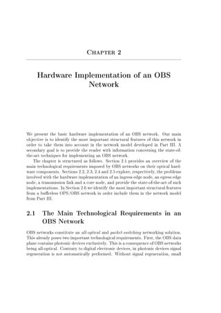
Figure 2.2 presents the main elements in the hardware implementation of an OBS
ingress edge node. We begin this section by explaining how the hardware imple-
mentation in Figure 2.2 matches the functional description of an ingress edge node
in Section 1.2.
Incoming IP packets are sorted by an IP router and sent to dierent burst
assembly units according to their destination (see 1 in Figure 2.2). Each burst
assembly unit contains an aggregation buer that collects IP packets until an
algorithm called the aggregation strategy decides to stop the aggregation process
(see 2 in Figure 2.2). When this happens, the contents of the aggregation buer
constitute the electronic version of a burst. At this point, the ingress edge node
electronically generates the header packet associated to the burst at the header
generation unit (see 3 in Figure 2.2). The ingress edge node sends the header
packet through the signaling wavelength channel at optical domain, waits a certain
oset time and then sends the contents of the aggregation buer as an optical burst
through the corresponding data wavelength channel (see 4 in Figure 2.2).
The IP routers, burst assembly units and header generation units in Figure 2.2
can be all implemented with digital electronics, and pose no challenge to current
technology. However, the transmission of information through the optical domain
requires the use of two photonic devices: fast tunable lasers and optical modulators
(see Figure 2.2). We now proceed to explain the basic functioning of a laser and
then introduce the state-of-the-art on fast tunable lasers which can be used in
OBS ingress edge nodes. At the end of this section we briey explain the basic
principles of optical modulation formats.
A laser consists in a gain medium inside an optical cavity, with a means to
supply energy to the gain medium. In its simplest form, the optical cavity consists
of two parallel mirrors arranged such that light bounces back and forth, each](https://image.slidesharecdn.com/3f7f65b2-eeec-4afd-a395-b25a5ff55a20-160530113535/85/Modeling_Future_All_Optical_Networks_without_Buff-41-320.jpg)
![2.2 Hardware Implementation of an Ingress Edge Node 15
photon in the same frequency (ωcav), phase, and direction (parallel to the cavity
axis) as the incident photons. This interaction is called the stimulated emission of
light, and gives rise to a coherent beam of light that is characteristic of a laser.
Nevertheless, it could also happen that some of the photons that are being
reected back and forth in the cavity mirrors, are absorbed by particles with
energy E1, instead of producing stimulated emission from particles with energy
E2. Therefore, an important condition in order to produce amplication of the
stimulated emission, is that the number of particles with energy E2 exceeds the
number of particles with energy E1. In that case, population inversion is achieved
and the amount of stimulated emission due to light that passes through is larger
than the amount of absorption. Hence, the light is amplied. Typically, one of
the two cavity mirrors, the output coupler, is partially transparent. Part of the
light that is between the mirrors (i.e., is in the cavity) passes through the partially
transparent mirror and appears as a narrow beam of light with a wavelength
λ = 2πc
ωcav
. This wavelength can be tuned by changing the optical path length
L, either by varying the refractive index n of the cavity medium or the cavity
length d [16]. In this case we have a tunable laser. We now briey describe the
state-of-the-art on tunable lasers which can be used in OBS networks.
The refractive index of the cavity medium can be changed by means of temper-
ature variations or current injection, whereas the cavity length can be changed by
using MEMS (Micro-Electro-Mechanical Systems) [10]. Temperature variations
leads to slow tuning devices, which cannot be used for OBS [16]. Fast tunable
lasers based on current injection or MEMS constitute promising candidates for
OBS. The most common current injection-based implementation is the multi-
section Distributed Bragg Reector (DBR) laser. Several working prototypes have
been implemented in the labs recently [146, 13, 137, 93, 6], and all of them have
exhibited tuning times in the range of ns. According to Section 2.1 the required
tuning time for OBS networks is in the range of µs, thus this gure is three orders
of magnitude below the OBS requirement. The most common MEMS-based im-
plementation is the External Cavity Laser (ECL). At least two working prototypes
have been implemented in the labs [11, 97] showing tuning times below 50 ns, also
suitable for OBS. Finally, Intune Technologies [85] commercializes in its AltoNet
series tunable lasers with tuning speeds between 50 and 200 ns. This is the only
example of a commercial tunable laser suitable for OBS that we have found.
OBS networks do not require specic optical modulators dierent from the
ones used in other optical networks. Thus, we now briey introduce the reader
to the basic concepts in optical signal modulation and refer to [4, 116] for de-
tails on this subject. The optical signal generated by a laser is analog in nature
and constitutes what we call the optical carrier signal. A carrier signal may be
thought of as a container to carry information across the network. In our case,](https://image.slidesharecdn.com/3f7f65b2-eeec-4afd-a395-b25a5ff55a20-160530113535/85/Modeling_Future_All_Optical_Networks_without_Buff-43-320.jpg)
![2.3 Hardware Implementation of an Egress Edge Node 17
(a) (b)
Figure 2.3: (a) Hardware implementation of an egress edge node. (b) Detailed
implementation of a burst mode receiver for OBS networks using an IM/DD mod-
ulation format.
cic burst-mode receivers. The internal structure of a typical burst mode receiver
is presented in Figure 2.3(b) [152, 145, 119, 48, 158] for the case of an IM/DD
modulation format. At a rst stage the optical burst is converted to the electronic
domain, usually by means of a photodiode. The detailed description of such de-
vices falls out of the scope of this chapter, since they are the same used in a normal
(i.e., non OBS) optical receiver. We refer to [4, 116] for details on this subject. The
output of the opto-electronic converter is an electronic analog signal, which is then
converted to a digital signal by means of an analog to digital converter (ADC) (see
Figure 2.3(b) ). This ADC has two quantization steps, that is, it provides a digital
output of one bit for each sampled value of the input analog signal. Moreover, it
is an adaptive ADC, since the size of the quantization steps is changed according
the to magnitude of the input signal.
In OBS networks a preamble precedes the transmission of each burst. This
preamble is just a sequence of bits containing no information, and it represents
a small fraction of the total burst length. Burst preambles are used by the clock
recovery unit to obtain the signal clock so that the analog signal can be sampled
for the ADC. The typical preamble duration in OBS networks is in the order of
µs (see Section 2.1). The clock recovery unit is needed since OBS networks are in
most cases asynchronous [135, 67]. In a synchronous network this clock recovery
unit is not needed because in this case the modulation and demodulation processes
at the ingress and egress edge nodes are coordinated by a global clock signal.
In an OBS network the optical signals corresponding to dierent bursts might
have traveled along dierent paths experiencing dierent losses and amplications
on their way. This implies that a receiver must be able to dynamically adapt to
such power level variations, which otherwise might severely increase the quantiza-
tion error at the ADC. This is done at the quantization adjustment unit, which](https://image.slidesharecdn.com/3f7f65b2-eeec-4afd-a395-b25a5ff55a20-160530113535/85/Modeling_Future_All_Optical_Networks_without_Buff-45-320.jpg)
![18 Hardware Implementation of an OBS Network
chooses an appropriate size for the quantization steps in the adaptive ADC in
Figure 2.3(b) according to the power level of the incoming burst.
Once the sizes of the quantization steps have been selected and the clock signal
has been recovered, the burst mode receiver can convert the analog signal into a
digital signal of zeroes and ones at the ADC. At the last stage of the burst mode
receiver, the dierent IP packets comprising the burst are extracted and sent to
the IP router for further forwarding through the Internet.
The design of burst mode receivers for other modulation formats is more com-
plex and implies in general the use of more photonic devices operating on the
optical signal before it reaches the opto-electronic converter. The main goal of
such additional devices is to convert the modulation of the optical carrier signal
(e.g. in phase, or polarization) into a modulation in intensity which can be de-
tected by the photodiode (i.e., by the opto-electronic converter) in Figure 2.3(b).
The rest of the elements in the gure are then basically the same.
In the last years several burst mode receivers have been demonstrated for 10
Gbps [145, 119] and for 40 Gbps [48]. In addition, some all-optical burst mode
receivers and clock recovery units have been experimentally demonstrated for 40
Gbps in [92] and [79], respectively.
2.4 Hardware Implementation of a Transmission
Link
The possibility to send great amounts of information through long distances at a
relatively low cost makes optical networks the natural choice to implement core
networks. Optical networks provide such possibility thanks to two main techno-
logical breakthroughs: dense wavelength-division multiplexing (DWDM) systems
and EDFAs [4, 116].
DWDM systems multiplex multiple optical carrier signals on a single optical
ber by using dierent carrier wavelengths. That is, one ber is transformed into
multiple virtual bers or wavelength channels which can transfer information in
parallel. Typical wavelength channel capacity values are 1 Gbps, 2.5 Gbps or
10 Gbps (40 Gbps in the near future) [106]. The number of wavelength channels
multiplexed in the same DWDM ber ranges from tens to a few hundred, providing
current DWDM bers with a total capacity in the terabit per second (or 1012
bits
per second) range.
The use of EDFAs allows to compensate the ber losses that take place along
a path for carrier wavelengths in the 1550 nm telecommunication window. All
multiplexed wavelength channels are simultaneously amplied in a single EDFA.
These EDFAs enable the construction of long-distance DWDM optical links at a](https://image.slidesharecdn.com/3f7f65b2-eeec-4afd-a395-b25a5ff55a20-160530113535/85/Modeling_Future_All_Optical_Networks_without_Buff-46-320.jpg)
![2.4 Hardware Implementation of a Transmission Link 19
relative low cost.
OBS networks are fully compatible with the DWDM technology [134, 135].
However, commercial EDFAs (or any other kind of doped ber ampliers) cannot
be directly used in OBS networks. Their use would produce large signal power
variations, signicantly increasing the BER [71, 125]. For this reason, we focus
in this section on this problem and study how to modify the basic design of an
EDFA in order to make it suitable for OBS networks, and leave aside the details
concerning the DWDM technology.
This section is structured as follows. First we begin with a description of the
operating principle of an EDFA in Section 2.4.1. We explain in Section 2.4.2 the
reason why a commercial EDFA could not be used in an OBS network. Finally,
in Section 2.4.3 we provide the state-of-the-art of the possible modications to
an EDFA which have been proposed in the literature in order to overcome the
problem mentioned in Section 2.4.2.
2.4.1 The Operating Principle of an EDFA
The operating principle of an EDFA is very similar to that of a laser, explained
in Section 2.2. In an EDFA, a section of the optical ber is doped with the rare
earth element erbium. A pump laser excites the erbium ions into a higher energy
level. Excited erbium ions interact with the photons from the optical signal and
decay back to a lower energy level via the stimulated emission of photons at the
signal wavelength. In the process of stimulated emission the number of photons
in the input signal is incremented and thus the signal is amplied. Together
with stimulated emission, the spontaneous emission of photons takes place in an
EDFA (see Section 2.2). Spontaneously emitted photons in the same direction and
wavelength as the optical signal get also amplied by the EDFA and represent its
main source of noise, the so-called amplied spontaneous emission (ASE).
2.4.2 The Problem of Using EDFAs in an OBS Network
The gain dynamics describe the time scale with which the gain reacts to changes
in the amplitude of the input signal or the pump. In an EDFA such dynamics
are relatively slow, typically in the order of ms [32]. In circuit-switching optical
networks, high bit rate intensity-modulated (IM) light changes its amplitude at a
rate below the ns scale. For instance, a 10 Gbps IM signal changes its amplitude
approximately every 0.1 ns. Thus, in circuit-switching optical networks the gain
of the EDFA is not aected by amplitude variations of the input signal. This
produces a nearly constant amplied output power and we say then that the gain
is stabilized.](https://image.slidesharecdn.com/3f7f65b2-eeec-4afd-a395-b25a5ff55a20-160530113535/85/Modeling_Future_All_Optical_Networks_without_Buff-47-320.jpg)
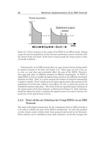
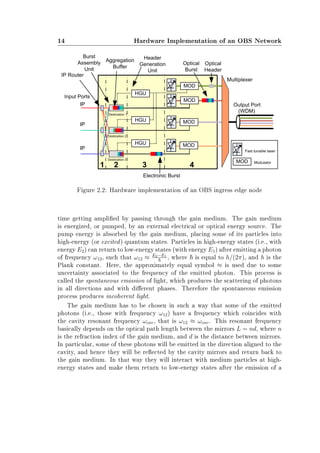
![2.4 Hardware Implementation of a Transmission Link 21
(a) (b)
Figure 2.5: (a) Forward EDFA gain control scheme. The control circuit works
with the power level of the input signal. (b) Feedback EDFA gain control scheme.
The control circuit works with the power level of the output signal.
power of the pump laser is adjusted to countermeasure the variations in the input
signal and the control entity is implemented electronically. In this category there
are two possible congurations. In the forward control conguration [71, 125] (see
Figure 2.5(a)), the control unit receives information concerning the power level
of the input signal. In the feedback control conguration [88, 47, 89, 155] (see
Figure 2.5(b)) it receives information concerning the power level of the output
signal.
In the second category an additional optical signal is introduced in the gain
band of the EDFA in order to countermeasure the variations in the input signal.
Again, the power of the signal introduced can be adjusted by measuring that of
the input signal in a forward (Figure 2.5(a))) or feedback (Figure 2.5(b)) congu-
ration. Additionally, in this case the feedback control scheme can be implemented
all-optically. This is called gain clamping, and has been widely studied in the
literature [30, 110, 181, 177, 100].
In the third category an extra WDM channel is used to compensate the vari-
ation of the total optical power [154, 150, 151]. The power of the extra channel
is adjusted to keep the total power of the extra channel and the signal channels
constant at the input of the EDFA. A promising candidate for this extra channel
in OBS networks would be the signaling channel that carries the header packets.
Because of the low data rates on this channel, it should be possible to design a
receiver which can tolerate the power variations introduced by the compensation
algorithm [16].](https://image.slidesharecdn.com/3f7f65b2-eeec-4afd-a395-b25a5ff55a20-160530113535/85/Modeling_Future_All_Optical_Networks_without_Buff-49-320.jpg)
![22 Hardware Implementation of an OBS Network
Figure 2.6: Generic OBS core node, courtesy of Siemens AG. HP stands for header
processing, HG for header generation, E/O for Electro-optical conversion, O/E for
opto-electronic conversion, and λ-conversion for wavelength conversion.
2.5 Hardware Implementation of a Core Node
In this section we present the main technological requirements needed in order
to implement an OBS core node, together with state-of-the-art solutions to meet
such requirements.
The main functionality of a core node is to switch and forward the optical
bursts as fast as possible and without causing large burst losses due to contention.
Since contention is one of the main concerns in OBS networks, the purpose of many
of the hardware elements in a core node is to reduce it. In general an OBS core
node comprises six main elements: an input interface, ber delay lines (FDLs), an
optical switch fabric, a wavelength converter unit, a control unit and an output
interface (see Figure 2.6) [134, 135].
At the input interface the wavelength channels are demultiplexed from the
WDM ber. The contents of the control channels are converted to the electronic
domain in order for the burst headers to be processed. After processing, the head-
ers are regenerated and converted back to the optical domain. The data channels
are fed into FDLs in order to regenerate the constant oset time existing between
each header packet and its associated burst (see Section 2.5.1). Then bursts are
switched through the optical switch fabric. At its output wavelength conversion](https://image.slidesharecdn.com/3f7f65b2-eeec-4afd-a395-b25a5ff55a20-160530113535/85/Modeling_Future_All_Optical_Networks_without_Buff-50-320.jpg)
![2.5 Hardware Implementation of a Core Node 23
takes place in order to adjust their wavelength to that of their corresponding out-
put wavelength channel. At the output interface control and data channels are
multiplexed back into a single WDM ber.
We now focus on the implementation of such a core node. The input and output
interfaces basically consist of a multiplexer and demultiplexer unit, respectively.
Such units are typical from DWDM systems and do not require any modication
for their use in OBS networks [116]. The control unit contains mainly standard
digital electronics, which do not represent a real challenge for nowadays technology.
Its associated photonic devices are of two types. First, the kind of opto-electronic
converter described in Section 2.3 to convert the optical header packets into the
electronic domain. Second, lasers to convert the packet headers back to the optical
domain. Such lasers do not need to be tunable (see Section 2.2), since the signaling
wavelength is xed for every outgoing ber. The main technological requirements
for the construction of an OBS core nodes are in the three remaining blocks: the
FDL, optical switch fabric and λ-conversion (also called wavelength conversion)
blocks. We discuss now in more detail the hardware components comprising each
one of these three blocks.
2.5.1 Fiber Delay Lines
Fiber delay lines (FDLs) are similar to electronic random access memories (RAMs)
in that they can delay the arrival of a burst. They basically consist in a long loop-
like ber over which a contending burst can be sent. The contending burst is
successfully sent through an available wavelength channel if contention is over
when it comes out from the FDL. Otherwise, the burst can be sent again through
the FDL, or it can be discarded, in which case the burst is blocked (i.e., lost). Thus,
unlike in RAMs, the delay introduced by FDLs is a multiple of a constant, which
is equal to the time it takes an optical signal to travel through the FDL. FDLs of
dierent lengths might be used in order to palliate to some extent the burst loss
due to contention. However, as stated in the introduction, most OBS core node
architectures avoid the use of FDLs to reduce burst loss [161, 172, 133, 65].
The use of FDLs seems to be justied in an OBS core node in order to re-
generate the oset time between header packet and burst. Indeed, header packets
are delayed at the core nodes with respect to their associated burst due to noneg-
ligible processing times at the electronic domain. Thus, the oset time between
the transmission of a header and its associated burst is reduced at each core node
visited. In order not to limit the number of hops a burst can travel, short and
relatively inexpensive FDLs may be use for oset regeneration purposes [134, 135].](https://image.slidesharecdn.com/3f7f65b2-eeec-4afd-a395-b25a5ff55a20-160530113535/85/Modeling_Future_All_Optical_Networks_without_Buff-51-320.jpg)
![24 Hardware Implementation of an OBS Network
2.5.2 OBS Switch Fabrics
The switch fabric plays a fundamental role in the design and construction of an
OBS core node. It also plays a very special role regarding the performance of the
network, since the switching fabric is actually where bursts are physically blocked
or lost. A burst is lost at the switch fabric when it is sent through a wavelength
channel in an outgoing link that is busy with the transmission of another burst.
Blocking is physically manifested as a loss of power from the optical signal repre-
senting the burst. The physical mechanism by which this power is lost depends on
the underlying technology used to implement the switching fabric. We shall see
later in this section an example of this mechanism in a switching fabric based on
SOA technology (see Figure 2.7).
Perhaps, the two most important characteristics of an OBS switch fabric are
that it is all-optical and that it is usually large (N · M × N · M switch fabrics are
needed for N input/output ports with M wavelength channels each). Due to their
size, the typical architecture of an OBS switch fabric comprises the interconnection
of a number of smaller switches, which we call basic switches. The functionality
of such basic switches is to enable that bursts entering on one input can access
any chosen output. OBS networks impose two specic requirements on the basic
switches. First, their switching times must be in the range of µs (see Section 2.1).
Second, they must show a very low insertion loss. The insertion loss represents
the fraction of signal power that is internally lost at the basic switch. This re-
quirement is fundamental for the construction of large optical switch fabrics since
the insertion loss limits the number of basic switches that can be interconnected
without intermediate signal amplication.
The rst requirement alone automatically discards many switching technolo-
gies, such as Optomechanical [162], MEMS [10], Thermo-optic [33, 128], liquid
crystal [149] and bubble [157], all of them exhibiting switching times in the range of
ms. The main technologies with switching times low enough for OBS are: Acousto-
optic switches with switching times around 3 µs [73], Electro-optic switches with
switching times below 10 ns [117, 34], and Semiconductor Optical Amplier (SOA)
switches with switching times around 1 ns [91].
The second requirement concerning the low insertion loss questions the use of
Acousto-optic and Electro-optic switches, which in the references provided show
insertion losses of 6 and 9 dB, respectively. Such relatively high losses can be
compensated with the use of additional ampliers, but this in turn increases the
manufacturing cost of the switch and introduces additional noise. Moreover, in [73,
117, 34] the crosstalk gure is around -35 dB, which is also considered to be
relatively high [16]. The conclusion here is that these hardware specications pose
serious problems for the manufacturing of large switch fabrics based on acousto-
optic and electro-optic technologies.](https://image.slidesharecdn.com/3f7f65b2-eeec-4afd-a395-b25a5ff55a20-160530113535/85/Modeling_Future_All_Optical_Networks_without_Buff-52-320.jpg)
![2.5 Hardware Implementation of a Core Node 25
Figure 2.7: Basic architecture of a 2x2 SOA-based switch. The control unit selects
which two SOA devices receive the pump current and which not.
SOA switches constitute perhaps the most promising candidate for building
large optical switch fabrics in OBS core nodes. With a switching time around 1 ns
they are fast enough for OBS networks (see Section 2.1). Moreover, due to inherent
amplication properties they show virtually no insertion loss and a crosstalk gure
below -50 dB [91].
The functioning of a SOA device is similar to that of an optical ber amplier
such as an EDFA. The main dierences are the material used (semiconductor
instead of doped ber) and the pump used to invert the population (electrical
instead of optical) [32]. The main dierence in behavior is in the gain dynamics.
Recall from Section 2.4 that in EDFAs the size of the inverted population (and thus
the gain) is sensitive to intensity variations in the input signal or laser pump that
take place in a temporal scale above the ms range. For this reason the gain of the
EDFAs does not vary with high bit rate signals. In SOAs the size of the inverted
population (and therefore the gain) reacts to variations in a temporal scale of the
order of a few hundreds of ps and above [32]. This makes SOAs inadequate for
in-line amplication, but useful for other applications such as switching.
In the basic SOA-switch conguration, there is a SOA per each pair of input-
output lines in the switch. In this context, a line can be either a wavelength
channel or an optical ber. The pumping current of the SOA of an output line is
turned on if the optical signal at the input line is switched through that line. In
this case the signal is amplied. The pumping current is turned o if the optical
signal at the input line is switched through another line. In this case the SOA
device absorbs the signal since no population inversion is achieved. Figure 2.7
presents this principle in the basic architecture of a 2 × 2 SOA-based switch. By
turning on the pumping current of one of the two rst SOAs in this gure and
by turning o the pumping current of the other SOA, the rst input ber can be](https://image.slidesharecdn.com/3f7f65b2-eeec-4afd-a395-b25a5ff55a20-160530113535/85/Modeling_Future_All_Optical_Networks_without_Buff-53-320.jpg)
![26 Hardware Implementation of an OBS Network
switched to any output ber. The same applies for the second input ber and
the third and fourth SOAs. The SOA may operate on entire input bers (as in
Figure 2.7), and on single wavelength channels (i.e., one SOA device per input
wavelength channel).
The high speed at which the SOA gain varies depending on the intensity of the
pump current enables to build fast switching devices. The amplication inherent
to a SOA enables it to exhibit very low insertion loss. This allows building large
switch fabrics by integrating SOAs with passive couplers like the one in Figure 2.7
and spares the use of additional EDFAs at the OBS core nodes. However, SOA
switches are far from being ideal. Their main problems are power consumption and
the noise introduced by the spontaneous emission of photons, or ASE. Crosstalk
also becomes an issue when a SOA device is used to amplify all channels in a
WDM ber. For this reason SOAs are usually connected to individual wavelength
channels, and not to whole input bers as in Figure 2.7 [58, 59, 16].
2.5.3 Wavelength Conversion
Full wavelength conversion basically allows a core node to switch between any
wavelength channel at any input ber and any wavelength channel at any output
ber. In order for this functionality to be present at a core node, wavelength
converters must be used. A good introduction to wavelength converters and further
references can be found in [116, Chapter 21].
The use of full wavelength conversion capabilities is perhaps one of the most
ecient contention resolution strategies in OBS networks [161, 46, 133, 45, 175,
174, 167]. Partial wavelength conversion uses a shared pool of wavelength con-
verters for all output ports of a switch. It can also reduce contention to some
extent, but its overall complexity can be higher than that of concepts with full
conversion [66, 54]. Thus, this work considers core node architectures with full
wavelength conversion exclusively.
The wavelength converters needed for a core node architecture like the one in
Figure 2.6 must be of the type variable-input xed-output. That is, they must be
capable of taking in a variety of wavelengths but need only to convert to a xed
output wavelength. One wavelength converter is needed per wavelength channel
per output port.
Regarding their implementation, there are two types of wavelength converters:
O/E/O and all-optical wavelength converters. In the O/E/O approach the signal
is converted to the electronic domain and sent back through the optical domain at
the desired output frequency. The O/E converters typically do not care about the
input wavelength, as long as it is in the 1550 nm window. The laser of the E/O
block is usually xed at an output wavelength. Thus, O/E/O converters fulll the
variable-input xed-output requirements from the architecture in Figure 2.6. In](https://image.slidesharecdn.com/3f7f65b2-eeec-4afd-a395-b25a5ff55a20-160530113535/85/Modeling_Future_All_Optical_Networks_without_Buff-54-320.jpg)
![2.6 Modeling Considerations 27
addition, signal regeneration (see Section 2.1) usually takes place at the electronic
domain. This spares the use of EDFAs to amplify the signal and eectively reduces
the noise level. Commercial O/E/O converters for transmission speeds up to 10
Gbps are already available [162, 84] and a bit rate up to 40 Gbps also seems to
be achievable [16]. The main problems with O/E/O converters are their price and
that they are not transparent to the bit rate and the modulation format of the
signal. This transparency is achieved by all-optical converters, which also promise
lower implementation costs. Currently several all-optical wavelength converters are
being subject of experimentation but are not mature enough for commercialization.
Such is the case of [87, 182, 148, 112, 178, 25].
2.6 Modeling Considerations
In this section we identify the most important structural features of buerless
OPS/OBS networks in order to take them into account in the network model
developed in Part III.
Transmission links in OBS and OPS networks consist in a number N of DWDM
bers. Each DWDM ber comprises a number L of wavelength channels, that
can be regarded as independent transmission channels (see Section 2.4). For this
reason, the analytical network model presented in Part III models a transmission
link as a number W = N · L of independent transmission channels.
In buerless OPS/OBS networks no FDLs are used in order to reduce the
blocking probability (see Section 2.5.1). For this reason, the analytical network
model presented in Part III assumes that contention necessarily implies the loss of
information (i.e., of packets or bursts).
In OBS networks, incoming bursts at a core node are directly forwarded to the
corresponding outgoing ber without any kind of delay due to buering, O/E/O
conversion, or processing (see Section 2.5). This operational principle is called cut-
through and is the opposite of the store and forward principle used in electronic IP
routers [156]. Standard OPS networks as presented in [108] OPS networks follow
the same operational principle at their core nodes. Thus, the analytical network
model presented in Part III assumes that core nodes are cut-through.](https://image.slidesharecdn.com/3f7f65b2-eeec-4afd-a395-b25a5ff55a20-160530113535/85/Modeling_Future_All_Optical_Networks_without_Buff-55-320.jpg)


![Chapter 3
Characterization of Highly-Aggregated
Internet Trac
This chapter presents a study of highly-aggregated IP trac as a representative
of the trac that will arrive at a typical OPS/OBS network. The main goal
is to address the current debate in the literature and determine whether highly-
aggregated IP trac can be best modeled with a Poisson or a long-range dependent
(LRD) process. For this purpose we analyze two lengthy and highly-accurate
trac traces provided by the Universitat Politècnica de Catalunya (UPC) within
the framework of the European-funded research projects NOBEL I and NOBEL
II [132, Deliverable 2.1]. Special emphasis is put on the concept of LRD, and the
result of applying well-known LRD estimators to the UPC trac traces.
The chapter is structured as follows. In Section 3.1 we motivate the problem
under study and present our methodology to solve it. Section 3.2 presents some
technical details concerning the measurement platform and the UPC trac traces
analyzed in this chapter. Section 3.3 presents the denition of a Poisson process,
its associated statistical tests, and the result of applying them to the UPC traf-
c traces. Section 3.4 provides an introduction to the wavelet transform, which
constitutes a useful tool for the study of LRD processes. Section 3.5 presents the
denition of an LRD process, its associated estimators, and the result of applying
them to the UPC trac traces. Section 3.6 presents a performance comparison
of dierent stochastic processes and the original UPC trac trace in two small
queuing scenarios, and presents the conclusion from this chapter.](https://image.slidesharecdn.com/3f7f65b2-eeec-4afd-a395-b25a5ff55a20-160530113535/85/Modeling_Future_All_Optical_Networks_without_Buff-59-320.jpg)
![32 Characterization of Highly-Aggregated Internet Trac
3.1 Problem Setting
As stated in the introduction, there is an important debate in the literature re-
garding the statistical nature of highly-aggregated trac in the Internet. Some
authors report the existence of LRD in Internet trac [107, 35, 126]. Other authors
maintain that highly-aggregated IP trac can be safely modeled with a Poisson
process [22, 23, 96]. This debate is important, since it is widely known that LRD
has a signicant negative impact on network performance, measured in terms of
such parameters as the buer dynamics and blocking probability [126, 63].
In this chapter we analyze the statistical properties of a set of trac traces
provided by the UPC. Our analysis contributes to the above-mentioned debate
substantially, since the UPC traces analyzed contain an unprecedented amount of
accurate data taken from a highly-aggregated transmission link.
We use the following methodology. First, we study with several tests the sta-
tistical nature of trac in these traces. The objective here is to decide whether
trac from the traces resembles more to a Poisson or to an LRD process. Second,
we t three trac models to the UPC traces and use them to synthesize arti-
cial trac traces. These trac models are a Poisson, an LRD and a Multifractal
model [140]. We then compare performance parameters in two simple queuing
scenarios using the synthesized and the original UPC traces. The objective here
is to decide whether trac from the traces behaves more like Poisson, LRD or
Multifractal trac.
3.2 The Measurement Platform
The trac traces analyzed in this chapter were provided by the Universitat Politèc-
nica de Catalunya (UPC) and were captured with the SMATRxAC measurement
platform [130]. We briey present in this section some details concerning this
platform and the traces captured, referred hereinafter to as the UPC trac traces.
The SMARTxAC measurement platform is a passive system that performs at
gigabit speeds without packet losses and with ns-precision in the packet time stamp
measurements. Anela Cientica is the Catalan RD network, managed by CESCA
and connects about 50 Universities and Research Centers in Catalonia. RedIRIS
is the Spanish RD network and connects Anela Cientica to the global Internet.
The point of measurement for the traces is a pair of Full-Duplex Gigabit Ethernet
links with a total capacity of 2 Gbps (see Figure 3.1).
The UPC trac traces comprise two traces with approximately 800 million
packets each. The rst trace contains the arrival times and sizes of the packets
traveling from Anela Cientica to RedIRIS in Figure 3.1, while the second contains
the arrival times of the packets traveling in the opposite direction. In what follows,](https://image.slidesharecdn.com/3f7f65b2-eeec-4afd-a395-b25a5ff55a20-160530113535/85/Modeling_Future_All_Optical_Networks_without_Buff-60-320.jpg)
![3.3 The Poisson Process 33
Figure 3.1: Measurement point for the UPC trac traces. Courtesy of UPC.
we refer to the rst and second traces as the uplink and downlink UPC traces,
respectively.
Due to the technical diculty of running statistical tests on a trace with 800
million samples, the uplink and downlink traces are divided in several segments
which are analyzed independently. The typical segment used contains 224
samples.
3.3 The Poisson Process
3.3.1 Denition
The homogeneous Poisson process of parameter λ is an arrival process such that
the interarrival times are independent and obey the exponential distribution [139]:
P[Interarrival time t] = e−λt
, where λ, t ∈ R+
. (3.1)
A renewal process is an arrival process such that the interarrival times are
independent and identically distributed, denoted as iid [139]. Thus, the Poisson
process is a particular case of renewal process for which the interarrival distribution
is exponential.
3.3.2 Testing the Poisson Hypothesis
In the literature on the statistical nature of IP trac traces the Poisson hypothesis
has been tested by means of various approaches. Most papers compute the auto-
correlation function of the packet interarrival time sequence, like [126, 22, 96]. A
few others use formal statistical tests, like [96]. In this section we have preferred](https://image.slidesharecdn.com/3f7f65b2-eeec-4afd-a395-b25a5ff55a20-160530113535/85/Modeling_Future_All_Optical_Networks_without_Buff-61-320.jpg)
![34 Characterization of Highly-Aggregated Internet Trac
to use the second approach since it is more formal and reliable. More specically,
we use two simple and yet powerful statistical tests borrowed from the Reliability
Theory [76] in order to test the Poisson hypothesis.
A Poisson process is a particular case of renewal process in which the interar-
rival time distribution is exponential. We use this fact in order to indirectly test
the Poisson hypothesis using the null hypothesis of a renewal process. For that
purpose we use the Lewis-Robinson (LR) and the Pair-wise Comparison Nonpara-
metric Test (PCNT) [76].
The LR and PCNT tests are dened as follows. Let T = {T1, . . . , TN } be
the sequence of N packet arrival times and X = {T2 − T1, . . . , TN − TN−1} the
sequence of interarrival times in the trace. The null hypothesis H0 in both tests
is that the observed sequence of packet interarrival times in the trace corresponds
to the sample path of a renewal process.
We begin with the LR test. Under the hypothesis of a renewal process and
conditioning on TN , the arrival times {T1, . . . , TN−1}, are uniformly distributed on
(0, TN ). The Lewis-Robinson statistic ULR is equal to
ULR =
N−1
i=1 Ti − (N − 1)TN
2
CV · TN
N−1
12
. (3.2)
In this equation CV is the coecient of variation that can be estimated as
CV =
√
σ2
X
X
, where σ2
X and X represent the variance and average estimators,
respectively. The test criterion is to reject H0 at the condence level α if ULR /∈
[−zα/2, zα/2]. We refer to the quantile zα/2 as the value for which P[Z zα/2] = α
2
,
where Z is distributed according to a standard normal distribution.
We present now the PCNT. Let U count the number of times that Xj Xi
for j i and for all i. Under H0 the mean value of U is E[U] = N(N−1)
4
and its
variance can be estimated as V ar[U] = (2N+5)(N−1)N
72
. According to the central
limit theorem for large N, U should be approximately distributed as a normal
distribution with mean E[U] and variance V ar[U]. Thus, the statistic:
UPCNT =
U − E[U]
V ar[U]
. (3.3)
should be approximately distributed as a standard normal distribution. There-
fore, the test criterion is to reject H0 if UPCNT /∈ [−zα/2, zα/2].
3.3.3 Results From the UPC Traces
Performing the LR and the PCNT tests with 10 uplink and downlink segments
of 223
arrival times (see Section 3.2) and a condence interval of 95% lead to a](https://image.slidesharecdn.com/3f7f65b2-eeec-4afd-a395-b25a5ff55a20-160530113535/85/Modeling_Future_All_Optical_Networks_without_Buff-62-320.jpg)
![3.4 Wavelet Transforms 35
rejection of the renewal process hypothesis. This implies a rejection of the Poisson
process hypothesis.
In our literature research, [96] was the only paper analyzing a trac trace
captured at a highly-aggregated optical link (i.e., a link with high capacity). In
particular, the link was an OC48 line, which has a capacity of about 2.5 Gbps.
However, the conclusion in [96] is the opposite; their statistical tests neither reject
the renewal process hypothesis, nor the exponential hypothesis for the packet
interarrival times. In other words, they conclude that highly-aggregated trac
does resemble a Poisson process.
These contradictory results could be explained in terms of the precision of the
measured packet arrival times. Indeed, in [96] the precision used was of µs, while
the UPC traces in our analysis have a precision of ns. In order to evaluate the
impact of the precision of the packet arrival times on the test results we performed
the following experiment. We rounded our traces to a precision of µs and run the
statistical tests once more. In this case, our test results did not reject the renewal
hypothesis, as in [96]. This suggests that an insucient precision in the packet
time stamps might have biased the statistical tests used in [96]. The result reveals
in any case the importance of having precise packet time-stamp measurements
when the level of aggregation of trac (i.e., its throughput) is high.
3.4 Wavelet Transforms
The next step after rejecting the Poisson hypothesis is to nd out whether the
UPC trac traces exhibit some kind of scaling properties, such as self-similarity or
LRD. Wavelet transforms constitute one of the best analytical tools for studying
stochastic processes with scaling properties. In this section we provide a short
introduction to the theory of wavelet transforms focusing on the discrete wavelet
transform (DWT). The material from this section is needed in order to understand
the Logscale Diagram, one of the main techniques used in this chapter to detect
scaling properties in the UPC traces. In addition, the wavelength transform theory
is used in Chapter 4 in order to study the behavior of OBS ingress edge nodes.
The structure of this section is the following. Section 3.4.1 gives a denition
of the DWT of deterministic functions while Section 3.4.2 provides the basic no-
tions from the multiresolution analysis (MRA) theory. Section 3.4.3 addresses the
computation of the DWT of stochastic processes.
The material from Section 3.4.1 is taken from [38, 114] while that from Sec-
tion 3.4.2 is taken from [111, 18]. The material from Section 3.4.3 is taken
from [127, 166].
Before proceeding with the introduction of the DWT we provide some basic no-
tions from the theory of functional analysis. Throughout Sections 3.4.1 and 3.4.2](https://image.slidesharecdn.com/3f7f65b2-eeec-4afd-a395-b25a5ff55a20-160530113535/85/Modeling_Future_All_Optical_Networks_without_Buff-63-320.jpg)
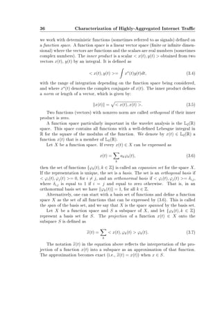
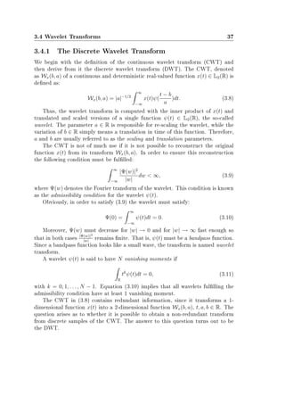
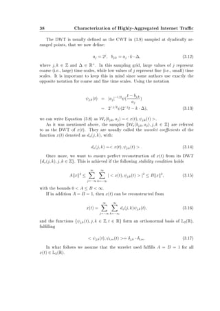
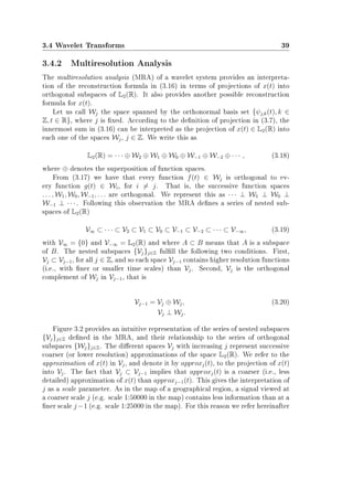
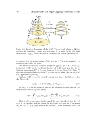
![3.4 Wavelet Transforms 41
projection approxj0 (t) of x(t) into Vj0 constitutes a representation of x(t) at scale
j0. The reminding projections into the spaces Wj, for −∞ j ≤ j0 contain the
details from x(t) lost when going from x(t) to approxj0 (t). In this representation
{ϕj0,k(t), k ∈ Z} are translates and re-scales of a scaling function ϕ(t), dened as
ϕj,k(t) = |2|−j/2
ϕ(2−j
t − k · ∆), (3.23)
with j, k ∈ Z, ∆ ∈ R+
. The set of functions {ϕj0,k(t), k ∈ Z} span the space
Vj0 . According to the MRA, the scaling function ϕ(t) is univocally dened by
the wavelet function ψ(t), and so are the spaces {Vj, j ∈ Z}. The coecients
{ax(j0, k), k ∈ Z} are the so called scaling coecients, and they are obtained from
ax(j, k) = x(t), ϕj,k(t) . (3.24)
In the representation of x(t) in Equation (3.22) the DWT comprises both, the
wavelet and scaling coecients. That is, {dx(j, k), j ≤ j0, k ∈ Z} and {ax(j0, k), k ∈
Z}, respectively. Thus, in this and the following chapter we will work with both
series of coecients when speaking about the DWT.
3.4.3 The Discrete Wavelet Transform of Stochastic Pro-
cesses
Wavelets were originally conceived for deterministic functions. Nevertheless, in
most cases they can be applied to stochastic processes as well. In particular, let
(Ω, β, P) be a probability space and let {Y (t), t ∈ R} a real-valued, continuous-
time, second-order process, i.e., {Y (t)} is jointly measurable and Y (t, w) is square
integrable in w ∈ Ω for each t ∈ R. Then, the DWT of {Y (t)} (i.e., {dY (j, k), j, k ∈
Z, j ≥ j0} and {aY (j0, k), k ∈ Z}) constitute two well-dened sequences of positive
(possibly correlated) random variables if the following condition on its autocorre-
lation function r(r, s) holds [20]:
R
r(u, u)|ψ(2j
u − k)|du ∞, (3.25)
for all j, k ∈ Z, where r(r, s) = E[Y (r)Y (s)].
Equation (3.25) turns out to be a rather mild condition fullled by many
stochastic processes of interest, such as self-similar processes [2, 164]. In what
follows we assume that Condition (3.25) holds for every stochastic process consid-
ered. Equalities such as dx(j, k) = x(t), ψj,k(t) in Equation (3.14) are to be
understood sample-wise.](https://image.slidesharecdn.com/3f7f65b2-eeec-4afd-a395-b25a5ff55a20-160530113535/85/Modeling_Future_All_Optical_Networks_without_Buff-69-320.jpg)
![42 Characterization of Highly-Aggregated Internet Trac
3.5 Self-Similar and Long-Range Dependent Pro-
cesses
Self-similar and Long-Range Dependent processes are by far the most important
scaling processes. They deeply lie in the foundations of the theory of scaling
processes and also nd useful applications in many practical problems, due to
their simple scaling law and low number of parameters.
3.5.1 Denition
Let us consider the discrete-time process {X[k], k ∈ Z}. In our trac modeling
context, X[k] represents the k-th interarrival time of the arrival process of packets
at, for instance, a link.
We say that {X[k]} is second-order stationary if E[X[k]] = µ does not depend
on k, and if its autocorrelation function r(w, s) = E[X[w]X[s]] satises translation
invariance, i.e., r(w+h, w) = r(h, 0), for all w, s, h ∈ Z. In second-order stationary
processes the autocorrelation function r(w+h, w) is usually written as r(h). Notice
that in such processes the second moment E[X[k]2
] is equal to r(0), for any k ∈ Z.
Thus, their variance does not depend on k either.
Let {X[k]} be a second-order stationary process with nite mean µ, nite
variance σ2
, and autocorrelation function r(h), h ≥ 0. For each m ∈ N we dene
the aggregated process {X(m)
[i], i ∈ Z} as
X(m)
[i] =
1
m
mi
k=m(i−1)+1
X[k], (3.26)
and we denote by r(m)
(h) its autocorrelation function.
The process {X[k]} is called exactly second-order self-similar with Hurst pa-
rameter H, 1/2 H 1 if for all m ∈ N,
r(m)
(h) = r(h), h ≥ 0, (3.27)
with
r(h) =
1
2
((h + 1)2H
− 2h2H
+ (h − 1)2H
). (3.28)
{X[k]} is called asymptotically second-order self-similar with Hurst parameter
H, 1/2 H 1 if for all h large enough,
r(m)
(h) → r(h), as m → ∞, (3.29)](https://image.slidesharecdn.com/3f7f65b2-eeec-4afd-a395-b25a5ff55a20-160530113535/85/Modeling_Future_All_Optical_Networks_without_Buff-70-320.jpg)
![3.5 Self-Similar and Long-Range Dependent Processes 43
with r(h) given by Equation (3.28) [107, 124]. Thus, second-order self-similarity
captures the property that correlation structure is exactly (condition (3.27)) or
asymptotically (the weaker condition (3.29)) preserved under time aggregation.
Intuitively, this is the most striking property of a second-order self-similar process,
since with other stochastic processes such as Markovian processes the correlation
structure of the process {X[m]
(k)} is degenerate as m → ∞, i.e., r(m)
(h) → 0 as
m → ∞ [107].
A second-order stationary process {X[k]} with nite mean and variance is
called long-range dependent (LRD) if its autocorrelation function is nonsummable.
That is,
∞
h=−∞
r(h) = ∞. (3.30)
Asymptotic or exact second-order self-similarity implies LRD since r(h) in
Equation (3.28) with 1/2 H 1 is nonsummable (see [124, 53] for details).
An essentially equivalent denition of LRD can be given in the frequency do-
main where the spectral density
Γ(ν) =
∞
h=−∞
r(h)e−ihν
, (3.31)
is required to satisfy the property
Γ(ν) ∼ cf |ν|−α
, as ν → 0, (3.32)
where cf is a nonzero constant, and 0 α 1 is related to the Hurst parameter
H through H = (α + 1)/2 [124].
3.5.2 The Logscale Diagram Estimator
The Hurst parameter plays a very important role in the denition of second-order
self-similar and LRD processes (see Equations (3.28) and (3.32)). This makes
the estimation of the Hurst parameter central to the study of such processes.
There are many estimators for the Hurst parameter. The most important ones
are the R/S method, the variance method, the periodogram method, the Logscale
Diagram (LD), the absolute value method, and the Whittle estimator (for details
see [94, 95]).
The LD estimator is one of the most complete and accurate estimators [94, 95].
It is based on the LD, which also can be used in order to detect the presence of self-
similar scaling behavior and LRD in the traces. Moreover, in Section 4.2 we use a
variant of the LD to study the second-order scaling properties of trac coming out](https://image.slidesharecdn.com/3f7f65b2-eeec-4afd-a395-b25a5ff55a20-160530113535/85/Modeling_Future_All_Optical_Networks_without_Buff-71-320.jpg)
![44 Characterization of Highly-Aggregated Internet Trac
from an ingress OBS edge node. For these reasons, in this section we describe the
LD in more detail, and explain how to detect and estimate second-order scaling
properties with it.
The LD is based on the DWT of the process to be analyzed. We begin by
presenting the main results concerning the DWT of exactly or asymptotically self-
similar processes (i.e., of LRD processes) and refer to [2] for details.
Let {X[k], k ∈ Z} be a second-order self-similar process. Then,
E[dX(j, k)2
] ∼ 2jα
· c, j → ∞, (3.33)
E[aX(j, k)2
] ∼ 2jα
· c, j → ∞, (3.34)
for some constant c ∈ R, and with 0 ≤ α ≤ 1, where α is related to H through
H = (α + 1)/2. Notice that the exponent of the power law in Equations (3.33)
and (3.34) is independent of the wavelet used. Also, the power law is the same
for the scaling and wavelet coecients. Taking base-2 logarithms in any of the
two equations leads to a linear equation in j with slope α. Thus, the power law in
Equations (3.33) and (3.34) suggests to plot in logarithmic scale of base 2 estimates
of E[dX(j, k)2
] or E[aX(j, k)2
] vs. the scale j in order to estimate α (and thus H)
in an LRD process by means of linear regression.
The scaling coecients {aX(j, k), j, k ∈ Z} inherit the LRD property from
the underlying process {X[k], k ∈ Z} [3]. Thus, the task of eciently estimating
E[aX(j, k)2
] from a single realization of {X[k], k ∈ Z} is extremely dicult due
to long-lasting correlations in the series {aX(j, k), j, k ∈ Z}. Fortunately, the esti-
mation of E[dX(j, k)2
] presents a quite dierent scenario. In fact, the correlation
between wavelet coecients {dX(j, k), j, k ∈ Z} at dierent locations (i.e., dier-
ent j and k) is controlled by the number of vanishing moments N in the mother
wavelet according to:
E[dX(j, k)dX(j , k )] ≈ |2−j
k − 2−j
k |α−1−2N
, |2−j
k − 2−j
k | → ∞. (3.35)
According to this equation, if N ≥ α/2 the correlations decay drastically and
the wavelet coecients are short-range dependent. In order to estimate the scaling
parameter α (or equivalently, the Hurst parameter H) we idealize this low corre-
lation and assume independence between wavelet coecients. This permits us to
use the time average
L2(j) =
1
m
m
k=1
dX(j, k)2
, (3.36)
as an estimator of the second moment E[dX(j, k)2
] of the wavelet coecients.
Numerical simulations show that the independence assumption reasonably holds](https://image.slidesharecdn.com/3f7f65b2-eeec-4afd-a395-b25a5ff55a20-160530113535/85/Modeling_Future_All_Optical_Networks_without_Buff-72-320.jpg)
![3.5 Self-Similar and Long-Range Dependent Processes 45
and that Equation (3.36) constitutes a good approximation of E[dX(j, k)2
][1, 2,
164].
Taking logarithms in Equation (3.33), we have that
log2E[dX(j, k)2
] ∼ jα + log2(c).
As we mentioned before, this strongly suggests a linear regression approach for
estimating α (and H through H = (α + 1)/2), which is the basic idea underlying
the LD estimator for second-order self-similarity proposed in [1]. Let us dene
S2(j) ≡ log2(L2(j)). Formally, we dene the LD as follows [1, 2, 142]:
Denition 3.5.1 The LD is a plot of the estimates S2(j) vs. the scale j, together
with 95% condence intervals about the S2(j).
The LD provides a means to visualize the second-order scaling structure of
data, which could for instance represent a sample path of a stochastic process
{X[k], k ∈ Z}. Second-order scaling behavior is not assumed, but detected through
the region of alignment, if any, observed in the S2(j) vs. j plot of the LD. By an
alignment region we mean a region of scales where, up to statistical variation, the
S2(j) values fall on a straight line as a function of j. More specically, it is a
region of scales {ja, . . . , jb}, with ja jb, where it is possible to draw a straight
line within the condence intervals of S2(j). Estimation of the scaling parameter α
can be performed through a weighted linear regression over the alignment region.
The weights in the linear regression are deterministic corrective factors needed in
order to correct some minor approximation errors in the LD. For more information
on this subject we refer to Section 1.3.2 in [1].
We now explain how to detect second-order scaling behavior with the LD. In
second-order self-similar (and therefore LRD) processes the alignment region is of
the form {j1, j1 + 1, . . .} (see Equation (3.33)). Since the amount of data analyzed
in any practical example must be nite, the alignment region for nite samples of
second-order self-similar processes is of the form {j1, j1 +1, . . . , jm}, with jm ∞.
Here, jm is the coarsest scale present in the data series, which is related to its
length (see Section 3.4). If such alignment region is observed in the LD with
j1 = 1, then exact second-order self-similarity is the most reasonable choice [1].
Otherwise, an alignment region of the form {j1, j1 +1, . . . , jm} with j1 1 suggests
asymptotic second-order self-similarity [1]. If the alignment region is of the form
{j1, j1+1, . . . j2}, with j2 jm then Equation (3.33) does not hold and the absence
of second-order self-similar scaling behavior is the most plausible conclusion. The
same conclusion can be reached if no alignment region is observed at all.
We illustrate the use of the LD with an example from the literature called
the Bellcore trac trace (BC trace in short). The BC trace has been used as a
reference in many studies related to the scaling properties of network trac. This](https://image.slidesharecdn.com/3f7f65b2-eeec-4afd-a395-b25a5ff55a20-160530113535/85/Modeling_Future_All_Optical_Networks_without_Buff-73-320.jpg)
![46 Characterization of Highly-Aggregated Internet Trac
Figure 3.3: Logscale Diagram of the Bellcore trac trace. S2(j) = log2 L2(j),
where L2(j) is given in Equation (3.36) and j represents the scale (octave in the
gure).
trace comprises the arrival times of about 1 million Ethernet packets, captured at
the Bellcore Morristown Research and Engineering facility, and it can be found
in [160] under the keyword BC-pAug89. The LD of the BC trace is plotted in
Figure 3.3.
The BC trace is a well-known example of a trace exhibiting second-order self-
similarity. This can be seen in Figure 3.3 from the existence of an alignment region
of the form {j1, j1 + 1, . . . , jm}, with jm = 16. This alignment region {9, . . . , 16}
is dened by the existence of a linear t, marked with a dash-dotted line, that
remains within the condence intervals for S2(j). Since j1 = 9 1 we conclude
that the particular form of second-order self-similarity observed in the BC trace is
asymptotic.
3.5.3 Results From the UPC Traces
In this section we assume that the measured trace of packet interarrival times
constitute the values of the sample path of a second-order stationary process with
nite variance. We check with the help of the Logscale Diagram (in short LD)
whether or not this process is an exact or asymptotic second-order self-similar](https://image.slidesharecdn.com/3f7f65b2-eeec-4afd-a395-b25a5ff55a20-160530113535/85/Modeling_Future_All_Optical_Networks_without_Buff-74-320.jpg)
![3.5 Self-Similar and Long-Range Dependent Processes 47
(a) (b)
Figure 3.4: Logscale Diagram for the (a) Downlink UPC trace and (b) Uplink UPC
trace. S2 = log2 L2(j), where L2(j) is given in Equation (3.36) and j represents
the scale.
(LRD) process. We also use the LD estimator, as well as ve other estimators in
order to estimate the value of the Hurst parameter once second-order self-similarity
(and LRD) is conrmed.
We now proceed to use the LD with the UPC trace to detect second-order self-
similar scaling behavior. Figures 3.4(a) and 3.4(b) present the LD of a segment of
224
interarrival times from the downlink and uplink traces, respectively. We refer
hereinafter to these as the downlink and uplink segments. In the downlink and
uplink segment, alignment is detected for large time scales suggesting asymptotic
second-order self-similarity and LRD. Alignment begins for larger (i.e., coarser)
scales than in the BC trace, but the LD diagram does not seem to degenerate
into a at curve, which would indicate the absence of second-order self-similarity.
Although the complexity of the DWT scales linearly with the number of data
samples [18], 224
seems to be the upper limit for our Matlab implementation of
the LD, and it is therefore the maximum segment size that we consider.
Figure 3.4 corresponds to a trace segment of approximately 25 seconds, while
the whole UPC trace comprises 1200 seconds (i.e., it contains 48 segments of
approximately 224
packets each). In order to check if the observed LRD and second-
order self-similarity is present in the whole trace, we present in the following gures
a LD for a signicant number of dierent segments taken at dierent positions
in the trace. In particular, Figure 3.5 presents the results for the downlink and](https://image.slidesharecdn.com/3f7f65b2-eeec-4afd-a395-b25a5ff55a20-160530113535/85/Modeling_Future_All_Optical_Networks_without_Buff-75-320.jpg)
![48 Characterization of Highly-Aggregated Internet Trac
Figure 3.5: Logscale Diagrams for dierent segments of the downlink UPC Trace.
Each subgure corresponds to a segment and represents approximately 25 seconds.
Figure 3.6 for the uplink directions. In both gures alignment of the LD is observed
within the condence intervals for most of the uplink and downlink segments (see
dash-dotted line). This is suggests that the observed second-order self-similarity
and LRD are present through all the trace.
Once detected the presence of asymptotic second-order self-similarity we pro-
ceed to the estimation of the corresponding Hurst parameter using the estimators
mentioned at the beginning of this section. Table 3.1 summarizes the results ob-
tained. The estimated Hurst parameter is lower for the downlink and uplink traces
compared to the BC one. However, one has to be careful when interpreting such
results. Due to the asymptotic nature of the self-similar phenomenon, not consid-
ering a suciently high number of scales in the analysis, or considering the lower
timescales may lead to biased estimations [60]. In our case, due to computational](https://image.slidesharecdn.com/3f7f65b2-eeec-4afd-a395-b25a5ff55a20-160530113535/85/Modeling_Future_All_Optical_Networks_without_Buff-76-320.jpg)
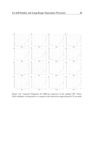
![50 Characterization of Highly-Aggregated Internet Trac
H Whittle C.I. LD C.I. AVM Periodogram Variance R/S
DL 0.5207 [0.5202, 0.5214] 0.972 [0.913, 1.07] 0.62 0.63 0.59 0.55
UL 0.5501 [0.5495, 0.5507] 0.876 [0.839, 0.953] 0.54 0.65 0.58 0.54
BC 0.6426 [0.6408, 0.6443] 0.752 [0.728, 0.777] 0.77 0.67 0.77 0.73
Table 3.1: Hurst parameter estimation for the interarrival time series (DL: down-
link trace, UL: uplink trace, LD: Logscale diagram, AVM: Absolute Value method
C.I.: condence interval)
constraints the length of the downlink and uplink traces used with all the estima-
tors was of 222
, except for the LD estimator, for which 24 scales were used (and
which provides a higher Hurst estimation). Since in the downlink and uplink traces
the asymptotic self-similar behavior begins at scales which are quite high (above
scale 15, see Figures 3.5 and 3.6), the analysis of an insucient number of scales
might account for the small values of H observed. In spite of this, all methods
used provide an estimation of the Hurst parameter above 0.5 for the downlink an
uplink traces, indicating the presence of asymptotic second-order self-similarity
and LRD.
3.6 Performance Evaluation
In the previous section we have concluded that the trac traces exhibit scaling
properties in the form of second-order self-similarity (and LRD). It remains to
study if the performance of these traces is due to their LRD nature, or if it can be
explained in terms of other statistical properties, such as for instance multifractal-
ity [55]. In other words, it remains to evaluate whether an LRD trac model can
accurately predict the performance that these traces might exhibit on a particular
network scenario.
In this section we focus on the performance of three trac models in two
dierent queuing scenarios. We chose the multifractal wavelet model (MWM)
as a representative of a trac model capable of capturing more complex scaling
behavior than self-similarity (see [140, Section III.D.]). As the second model we use
the MWM Beta model, a variant of the MWM capable of generating asymptotic
second-order self-similar, that is LRD, trac [140]. We refer to this self-similar
model by the SS acronym . As the third model we consider the Poisson process in
order to evaluate its usefulness as an approximate but simple trac model.
We chose two dierent queuing scenarios in order to benchmark the dierent
trac models: a single-server innite-buer node, and a multi-server buerless
node. In the rst scenario we are interested in the queuing behavior. This scenario](https://image.slidesharecdn.com/3f7f65b2-eeec-4afd-a395-b25a5ff55a20-160530113535/85/Modeling_Future_All_Optical_Networks_without_Buff-78-320.jpg)
![3.6 Performance Evaluation 51
may be representative of today's SDH (SONET)-based optical networks networks.
Indeed, in SDH networks buering at the core nodes takes place at the electronic
domain. Since electronic buers can be relatively large they could be modeled with
an innite-buer node. In the second scenario our aim is to measure the blocking
probability of the dierent traces. This scenario may be representative of future
buerless OPS/OBS networks.
All three trac models (MWM, SS and Poisson) are tted to the original up-
link and downlink traces, and are used in order to generate synthetic trac traces
representing packet arrival times. These traces are considered in a simulative study
together with the original uplink and downlink traces from UPC in order to com-
pare their behavior in terms the above mentioned performance parameters. We
want to focus on the ability of the three models to capture the relevant informa-
tion from the original uplink and downlink packet arrival time sequences in order
to predict performance parameters of interest. Thus, we use iid exponentially
distributed packet sizes in all simulation runs for all trac traces (including the
original downlink and uplink) in order to eliminate the eect of possible cross-
correlations between the packet arrival and packet size sequences. The gures
in the following sections present the results averaged for 16 simulation runs of 224
samples each, and with a link load of 50%. The 95% condence intervals are rather
small and they are not shown in Figure 3.7 for convenience.
Figures 3.7.a and 3.7.b provide the results concerning the blocking probability
of the traces from the dierent models in a buerless multiserver node. As it can
be observed, models which incorporate scaling (MWM and SS) lead to a good
approximation for the blocking probability. The use of the Poisson model implies
nonnegligible approximation errors in most practical situations. For instance, for
an OBS node with 6 wavelengths (a wavelength can be modeled as a server) the
error is of 1 order of magnitude, and it grows in a nonlinear fashion with increasing
number of wavelengths.
Figures 3.7.c and 3.7.d illustrate the results concerning the buer occupation
level. In particular, these gures plot the marginal probability that the buer
occupation level Q surpasses a threshold x for the downlink and uplink directions.
As it can be observed the Poisson model underestimates this performance measure,
while the SS model overestimates it. The MWM seems to provide results more in
accordance with those from the original BC trace. We have observed that for high
link loads (i.e., above 40%) the SS model overestimates the results, while for low
loads it underestimates them. Analogous results have been reported in [63].
Our results from Section 3.5 suggest that highly-aggregated IP trac presents
LRD. The results from this section suggest that LRD trac processes can accu-
rately predict the performance in terms of blocking probability in a simple buer-
less queuing system, but not the performance in terms of buer occupation level](https://image.slidesharecdn.com/3f7f65b2-eeec-4afd-a395-b25a5ff55a20-160530113535/85/Modeling_Future_All_Optical_Networks_without_Buff-79-320.jpg)
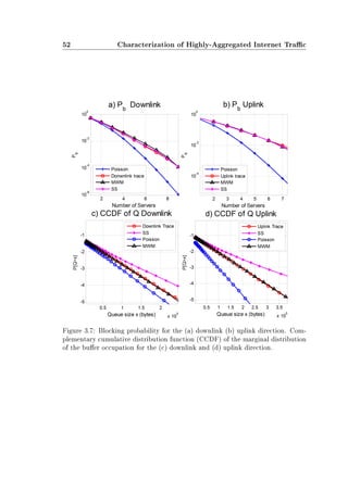


![Chapter 4
Trac Entering the Optical Domain in a
Buerless OPS/OBS Network
In Chapter 3 empirical evidence was gathered indicating the presence of LRD in
the highly-aggregated IP trac at the entrance of the ingress edge nodes of an
OBS/OPS network. This is particularly important since numerous empirical stud-
ies suggest that LRD negatively aects many network performance parameters,
like the blocking probability [126, 63]. For this reason, in this chapter we focus on
LRD and study whether this property can be found at the exit of the ingress edge
nodes of a buerless OBS/OPS network, whenever it is present in the IP trac at
their entrance.
This chapter is structured as follows. In Section 4.1 we briey state the problem
under study. Section 4.2 presents a new framework for the study of the impact of
the dierent OBS aggregation strategies (ASs) on the LRD of input trac. This
framework makes use of a new theoretical version of the Logscale Diagram (LD)
presented in Section 3.5.2. In Sections 4.3 and 4.4 we study the impact on LRD of
the Packet Count and the Buer Limit ASs, respectively, using both an analytical
and an experimental approach. Sections 4.5 and 4.6 present the same study for the
Timeout and Mixed ASs using an experimental approach exclusively. Section 4.7
presents the main modeling considerations from Part II of this thesis to be taken
into account by the stochastic network model presented in Part III.](https://image.slidesharecdn.com/3f7f65b2-eeec-4afd-a395-b25a5ff55a20-160530113535/85/Modeling_Future_All_Optical_Networks_without_Buff-83-320.jpg)
![56
Trac Entering the Optical Domain in a Buerless OPS/OBS
Network
4.1 Problem Setting
In an OPS network, incoming IP trac is sent through the optical domain as it
arrives at the ingress edge nodes. An immediate implication from this is that
LRD is present at the exit of the ingress edge nodes (i.e., in the optical domain)
whenever it is present at their entrance (i.e., in the electronic domain). Thus, we
conclude from the results in Chapter 3 that the analytical model from Part III
should take LRD into account when it is used to model a buerless OPS network.
The rest of this chapter is dedicated to the study of the case where the optical
network is a buerless OBS network.
When LRD network trac arrives at an ingress OBS edge node, the question
that arises is whether trac at its exit inherits such LRD or not. This question
arises because trac is shaped at the OBS ingress nodes through aggregation
strategies (ASs) that can potentially modify the statistical properties of incoming
IP trac by aggregating IP packets into bursts (see Section 1.2). Moreover, since
there are four main ASs described in the literature the answer to this question
depends on which AS is actually being used at the ingress edge nodes [179, 69,
39, 172]. As stated in the Introduction, the question has already received much
attention in the literature in the case when ingress edge nodes implement the
Timeouts AS [69, 86, 179, 8, 78, 153]. We complete the picture here by extending
the study to the Packet Count, Buer Limit and Mixed ASs.
Let us consider a burst assembly unit (see Section 2.2) inside an ingress edge
node in an OBS network receiving IP packets with interarrival times governed by a
discrete-time stochastic process {X[k], k ∈ Z}. According to the evidence gathered
in Chapter 3 we assume that the process {X[k], k ∈ Z} is LRD. Moreover, let the
discrete-time stochastic process {Y [k], k ∈ Z} represent the burst interarrival times
at the output of the burst assembly unit under study. That is, at the output of
the ingress OBS edge node.
The objective of this chapter is to study the second-order scaling structure
of {Y [k], k ∈ Z} (i.e., its LRD) for dierent ASs and to compare it with that
of {X[k], k ∈ Z}. We address the problem by using simulation studies and also
analytically, whenever it is possible. The main tool used in the simulative studies
is the Logscale Diagram (LD) introduced in Section 3.5.2 with the Daubechies
3 wavelet family [38]. The main tool used in the analytical studies is a novel
theoretical version of the LD that we refer hereinafter to as the Theoretical Logscale
Diagram (in short TLD).
In the simulation studies, the scenario is a burst assembly unit implementing
each one of the four basic ASs: Packet Count, Timeouts, Buer Limit and Mixed.
As an input for the burst assembly unit we use the packet arrival times and the
packet sizes from the UPC DL trace (i,.e., in the downlink direction; see Sec-](https://image.slidesharecdn.com/3f7f65b2-eeec-4afd-a395-b25a5ff55a20-160530113535/85/Modeling_Future_All_Optical_Networks_without_Buff-84-320.jpg)
![4.2 The Theoretical Logscale Diagram 57
tion 3.2). The objective is to measure from the simulation the burst interarrival
times at the output of the burst assembly, which are interpreted as a sample path
of {Y [k], k ∈ Z}. The burst interarrival times are then used in order to compute
the LD and to study the LRD of the burst arrival process at the OBS network.
The analytical studies use the same scenario but focus on the Packet Count and
the Buer Limit ASs. The objective is to relate the second-order scaling structure
of {Y [k], k ∈ Z} to that of {X[k], k ∈ Z} in order to be able to assess how LRD is
modied by the corresponding AS.
4.2 The Theoretical Logscale Diagram
In this section we present our novel theoretical logscale diagram (TLD in short).
As it will become clear from our description, the TLD is related to the standard
LD, although it diers from it in a number of signicant aspects. We begin by
introducing the well-known Haar wavelet ψ(t). This wavelet denes a scaling
function ϕj,k(t) of the form:
ϕj,k(t) =
2−j/2
2j
k ≤ t 2j
(k + 1)
0 Otherwise,
(4.1)
The TLD of a stochastic process {X[k], k ∈ Z} is based on the scaling coe-
cients obtained from its Haar wavelet transform. More specically:
Denition 4.2.1 The TLD of a process with Haar scaling coecients {aX(j, k),
j, k ∈ Z} consists in the plot log2(E[aX(j, k)2
]) vs. j, with j ∈ Z.
This denition is similar to the LD presented in Denition 3.5.1 in many as-
pects. The main dierence is that the LD works with real data, interpreted as a
realization of a processes {X[k], k ∈ Z}, while the TLD works with the whole pro-
cess {X[k], k ∈ Z} and not a sample of it. Thus, in the LD the main objective is to
obtain reliable results by working with good estimators, whereas in the TLD the
main objective is the simplicity of the analysis. This explains two further dier-
ences. First, the LD uses the wavelet coecients {dX(j, k), j, k ∈ Z} whereas the
TLD works with the scaling coecients {aX(j, k), j, k ∈ Z} exclusively. Both series
of coecients are eligible for the study of LRD since according to Equations (3.34)
and (3.33) their second moment exhibit a power law for LRD processes. As ex-
plained in Section 3.5.2, the wavelet coecients are the natural choice for the LD
because they lead to estimators with good properties if the number of vanishing
moments of the chosen wavelet is suciently high. In the TLD there is no need
to chose coecients with good estimation properties, but rather coecients that](https://image.slidesharecdn.com/3f7f65b2-eeec-4afd-a395-b25a5ff55a20-160530113535/85/Modeling_Future_All_Optical_Networks_without_Buff-85-320.jpg)
![58
Trac Entering the Optical Domain in a Buerless OPS/OBS
Network
lead to more simple analytical expressions. This turns out to be the case for the
scaling coecients.
Second, the LD works with a wavelet family with a number N ≥ 2 of van-
ishing moments whereas the TLD works with the Haar wavelet, which only has
1 vanishing moment [18]. Once more, the requirement in the LD for a wavelet
family with N ≥ 2 vanishing moments is motivated by the necessity to have good
estimators. Recall from Section 3.5.2 that the power law form of Equation (3.34)
does not depend on the wavelet chosen. Thus, for convenience the TLD is based
on the simplest wavelet ψ(t): the Haar wavelet (see Equation (4.1)).
There is a further dierence between the way we use in this chapter the TLD
and the LD, which is connected to the so-called initialization problem [165]. The
TLD and LD of the process {X[k], k ∈ Z} are based on the computation of its
DWT. This presents a problem, since the DWT is dened for continuous-time
stochastic processes (see Section 3.4.1), while {X[k], k ∈ Z} is a discrete-time
stochastic process. The most common approach to solve this problem is to dene
a continuous-time process {X(t), t ∈ R+
} that presents similar properties to those
that we want to study in {X[k], k ∈ Z}, and then to compute the DWT from it.
The LD usually employs a particular denition of {X(t), t ∈ R+
} presented
in [165]. This denition is very accurate since it provides a continuous-time ver-
sion {X(t), t ∈ R+
} with the same spectral density (see Equation (3.31)) than
{X[k], k ∈ Z} at frequencies close to zero. Since LRD is a property that refers to
the behavior of the spectral density at small frequencies (see Section 3.5.1), the
LRD of {X[k], k ∈ Z} is entirely reproduced in {X(t), t ∈ R+
}.
In the TLD we focus on analytical tractability and use a simpler approach
which consists in dening {X(t), t ∈ R+
} with the help of Dirac delta functions
δ(t) as:
X(t) ≡
∞
m=−∞
X[m]δ(t − m). (4.2)
This approach is shown in [165] to lead to small errors at the nest scales.
Since we want to study LRD, we are interested only in the asymptotic behavior at
large scales, which justies the use of Equation (4.2). In the numerical analysis we
make in this chapter we use the LD with the denition of {X(t), t ∈ R+
} presented
in [165], and validate the analytical results that use the TLD with the denition
of {X(t), t ∈ R+
} from Equation (4.2).
From Equation (3.34) we have that the TLD of the LRD IP packet interarrival
times {X[k], k ∈ Z} follows a line of slope α for j ≥ j1 (see Section 3.5.2). If
{X[k], k ∈ Z} is exactly second-order self-similar, then j1 = −∞, indicating that
the power law in Equation (3.34) applies for all j ∈ Z. If {X[k], k ∈ Z} is
asymptotic second-order self-similar, then j1 −∞.](https://image.slidesharecdn.com/3f7f65b2-eeec-4afd-a395-b25a5ff55a20-160530113535/85/Modeling_Future_All_Optical_Networks_without_Buff-86-320.jpg)
![4.3 The Packet Count Aggregation Strategy 59
According to Equation (4.2) we can express the scaling coecient aX(j, k) of
{X(t), t ∈ R+
} as
aX(j, k) = X(t), ϕj,k(t) =
∞
−∞
∞
m=−∞
X[m]δ(t − m)ϕj,k(t)dt.
From the particular form of the scaling function ϕj,k(t) in the Haar wavelet
(see Equation (4.1)) this expression simplies to:
aX(j, k) = 2−j/2
2j(k+1)−1
m=2jk
X[m]. (4.3)
We proceed now to study the second-order scaling structure of the burst inter-
arrival process for the dierent ASs in order to nd out how they transform the
LRD associated to the IP packet arrival process.
4.3 The Packet Count Aggregation Strategy
In the aggregation strategy with Packet Count the number of packets arriving at
the Burst Assembly Unit presented in Section 2.2 is counted. When the packet
count reaches a predetermined number, the packets in the aggregation buer are
assembled into a burst.
Let us assume that the burst assembly unit under study implements the Packet
Count AS. We begin with the analytical study and compute the TLD of the burst
interarrival time process {Y [k], k ∈ Z} at the exit of the burst assembly unit when
the packet interarrival time process {X[k], k ∈ Z} at the entrance is LRD.
The Packet Count AS generates bursts comprising a constant number N of IP
packets, N ∈ N+
. Thus, the burst interarrival times follow:
Y [m] =
N(m+1)−1
s=N·m
X[s]. (4.4)
Then, the following theorem holds
Theorem 4.3.1 The Haar scaling coecients {aX(j, k), j, k ∈ Z} of {X[k], k ∈
Z} and {aY (j, k), j, k ∈ Z} of {Y [k], k ∈ Z}, are such that:
aY (j, k) =
√
N · aX(j + log2 N, k), (4.5)
for j, k ∈ Z.](https://image.slidesharecdn.com/3f7f65b2-eeec-4afd-a395-b25a5ff55a20-160530113535/85/Modeling_Future_All_Optical_Networks_without_Buff-87-320.jpg)
![60
Trac Entering the Optical Domain in a Buerless OPS/OBS
Network
Proof: According to Equation (4.3) the Haar scaling coecients {aY (j, k), j, k ∈
Z} of {Y [k], k ∈ Z} are given by:
aY (j, k) = 2−j/2
2j(k+1)−1
m=2jk
Y [m].
Substituting Y [m] from Equation (4.4) gives:
aY (j, k) = 2−j/2
2j(k+1)−1
m=2jk
N(m+1)−1
s=N·m
X[s].
Integrating both sums into one and using j = log2N, j ∈ R+
yields:
aY (j, k) = 2−j/2
2(j+j )(k+1)−1
m=2(j+j )k
X[m].
Multiplying by 2j /2
· 2−j /2
and identifying aX(j, k) from Equation (4.3) leads
to
aY (j, k) = 2j /2
· aX(j + j , k).
In general j is not an integer, but technically speaking this does not pose any
problem since from Section 3.4.1 we have that the DWT coecients can be sampled
from the continuous CWT coecients at any point, not just at the integers. Thus,
aX(j, k) is indeed well-dened for j, k ∈ R.
Substituting N = 2j
yields Equation (4.5) and concludes the proof.
The following corollary is a consequence of this theorem.
Corollary 4.3.2 Let N be the number of IP packets per burst, and j = log2(N).
If {X[k], k ∈ Z} is exactly or asymptotic second-order self-similar with cuto
parameter j1 and Hurst parameter H, then {Y [k], k ∈ Z} is exactly or asymptotic
second-order self-similar with cuto parameter j1 − j and Hurst parameter H.
Proof: If {X[k], k ∈ Z} is asymptotic second-order self-similar with cuto pa-
rameter j1 then according to Equation (3.34) we have that log2 E[aX(j, k)2
] scales
linearly with j for j ≥ j1. That is, for j ≥ j1 we have
log2 E[aX(j, k)2
] = c + jα, (4.6)
where c is a constant.
Equation (3.34) (and thus, Equation (4.6)) are independent of the wavelet used.
We use the Haar wavelet and compute now the TLD of {Y [k], k ∈ Z}. That is,](https://image.slidesharecdn.com/3f7f65b2-eeec-4afd-a395-b25a5ff55a20-160530113535/85/Modeling_Future_All_Optical_Networks_without_Buff-88-320.jpg)
![4.3 The Packet Count Aggregation Strategy 61
we plot log2 E[aY (j, k)2
] vs. j. From the use of Equation (4.6) and Theorem 4.3.1
we have for j ≥ j1 − j that:
log2 E[aY (j, k)2
] = c + j (α + 1) + jα. (4.7)
That is, the TLD of {Y [k], k ∈ Z} for j → ∞ is equal to the TLD of {X[k], k ∈
Z} shifted up j (α + 1) units and with a cuto shifted left j scales. From this
we conclude that {Y [k], k ∈ Z} is asymptotic second-order self-similar with cuto
parameter j1 − j . Moreover, the slope α of the plot log2 E[aY (j, k)2
] vs. j for
j ≥ j1 − j is exactly the same as that of the plot E[aX(j, k)2
] vs. j for j ≥ j1.
From this we deduce that the Hurst parameter associated to {X[k], k ∈ Z} and
{Y [k], k ∈ Z} is the same.
If {X[k], k ∈ Z} is exactly second-order self-similar then the cuto parameter
is j1 = −∞. Since N ∞ we have that j ∞. Then, a similar argument as
for the asymptotic case leads to the conclusion that {Y [k], k ∈ Z} is also exactly
second-order self-similar with the same Hurst parameter H.
Thus, we may draw the following conclusions. Exactly and asymptotic second-
order self-similarity is not altered by the Packet Count AS. If N is the number of
packets per burst then in the asymptotic case the cuto scale j1 is shifted to the
left j units, with j = log2(N). This left-shifting simple means that the scaling
behavior typical from a second-order self-similar process starts at a ner scale for
{Y [k], k ∈ Z} than for {X[k], k ∈ Z}. In the exactly and asymptotic second-order
self-similar cases the value H of the Hurst parameter is preserved by the Packet
Count AS.
We proceed now to present the simulation results from a burst assembly unit
implementing the Packet Count AS. Figure 4.1 shows the LD of the burst interar-
rival times at the exit of the burst assembly unit for dierent values of j , where
N = 2j
is the number of packets per burst used in the simulation.
Recall from Section 3.5.2 that the cuto scale is the smallest scale j1 from which
the LD aligns within the condence intervals up to the largest scale present in data.
In Figure 4.1 we show this alignment with a dot-dashed line. In Section 3.5.3
it was shown that the UPC trace is LRD with a cuto scale of j1 = 15. From
Figure 4.1 we observe by looking at the beginning of the dash-dotted lines, marked
with black dots, that the burst interarrival times at the exit of the Packet Count
AS with 2j
packets per burst are LRD with a cuto parameter at scale j1 −
j . Moreover, the fact that the dash-dotted lines are parallel indicates that the
estimated value of α, and thus of the Hurst parameter H, is the same for the output
process {Y [k], k ∈ Z} with dierent number 2j
of packets per burst than for the
input process {X[k], k ∈ Z}. These two results are in perfect accordance with
Corollary 4.3.2, showing that the dierent solution to the initialization problem
used in the TLD and the LD does not seem to play a decisive role. We observe in](https://image.slidesharecdn.com/3f7f65b2-eeec-4afd-a395-b25a5ff55a20-160530113535/85/Modeling_Future_All_Optical_Networks_without_Buff-89-320.jpg)
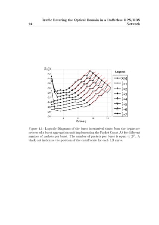
![4.4 The Buer Limit Aggregation Strategy 63
addition that for increasing values of j each LD curve is shifted up approximately
(1+α) units (α is close to one in this trace) with respect to the previous LD curve,
which gives Figure 4.1 a staircase appearance. This is a direct consequence of the
term j (α+1) in the sum of Equation 4.7, which shifts up the TLD exactly (1+α)
units with each increasing value of j .
4.4 The Buer Limit Aggregation Strategy
In the Buer Limit aggregation strategy there is a threshold B (in bits) in the
buer of the Burst Assembly Unit in Section 2.2. When the sum of the bits of the
packets collected in the buer crosses this threshold B the contents of the buer
are assembled into a burst.
Let us assume that the burst assembly unit under study implements the Buer
Limit AS. We begin with the analytical study and compute the TLD of the process
{Y [k], k ∈ Z} at the exit of the burst assembly unit when the process {X[k], k ∈ Z}
at the entrance is LRD.
In the Buer Limit AS the number of IP packets per burst is not a constant
anymore and depends on the size of the IP packets arriving at the edge node. In
this section we use the same principle from the analysis of the Packet Count AS
for the case in which the number of IP packets in the k-th burst is described by a
stochastic process {N[k], k ∈ Z}. The problem does not seem to lead to suitable
closed-form analytical expressions, and therefore an approximation is used. Its
empirical validation can be found at the end of this section.
We describe now the nature of this approximation. It is a common practice in
trac modeling to assume that the IP packet sizes {S[k], k ∈ Z} are independent
(see for instance [37] and references therein). This assumption is based on numer-
ous empirical studies, such as [22]. We make hereinafter this assumption, which
allows to establish the following theorem. Because of the independence assumption
needed, we treat the results derived from Theorem 4.4.1 as an approximation.
Theorem 4.4.1 Assume that the IP packet sizes are independent. If {X[k], k ∈
Z} is LRD with Hurst parameter H, then {Y [k], k ∈ Z} with the Buer Limit AS
is LRD with Hurst parameter H.
Proof: In the Buer Limit AS the number of packets per burst {N[k], k ∈ Z} de-
pends exclusively on the packet sizes {S[k], k ∈ Z} and the size of the aggregation
buer. Since successive packets have independent sizes, we have that successive
burst sizes are independent. Accordingly, we dene N as the random variable de-
scribing the number of packets inside any of these bursts. Applying Theorem 4.3.1
we have:](https://image.slidesharecdn.com/3f7f65b2-eeec-4afd-a395-b25a5ff55a20-160530113535/85/Modeling_Future_All_Optical_Networks_without_Buff-91-320.jpg)
![64
Trac Entering the Optical Domain in a Buerless OPS/OBS
Network
E[aY (j, k)2
] = E[N · aX(j + log2 N, k)2
],
with j, k ∈ Z.
Moreover in the Buer Limit AS the number of packets per burst {N[k], k ∈
Z} is independent of the packet interarrival times {X[k], k ∈ Z}. Therefore,
N is independent of {aX(j, k), j, k ∈ R}, since the last depends exclusively on
{X[k], k ∈ Z} (see Equation (4.3)). From this we may condition on N and write:
E[aY (j, k)2
] =
∞
n=1
nP[N = n]E[aX(j + log2 n, k)2
]. (4.8)
For j → ∞ using the fact that {X[k], k ∈ Z} is LRD (see Equation (3.34)) we
have
E[aY (j, k)2
] =
∞
n=1
nP[N = n]2(j+log2 n)α
,
which simplies to
E[aY (j, k)2
] = 2jα
E[N(1+α)
].
From this it follows that the TLD of {Y [k], k ∈ Z} has the same slope α as the
TLD of {X[k], k ∈ Z} for j → ∞. In other words, {Y [k], k ∈ Z} is also LRD with
the same Hurst parameter H = (α + 1)/2.
We proceed now to present the simulation results from a burst assembly unit
implementing the Buer Limit AS. Recall from Section 4.1 that the original packet
sizes from the UPC DL trace are used in the simulation.
Figure 4.2 shows the LD of the burst interarrival times at the exit of the
burst assembly unit for dierent values of j , where 2j
is the marginal average
number E[N] of packets per burst used in the simulation. In this AS we have that
E[N] = B/µ [39], where B is the buer size used in the simulation and µ is the
marginal average packet size computed from the trace.
In Figure 4.2 we show alignment within the condence intervals with a dot-
dashed line. The fact that the dot-dashed lines are parallel indicates that the
estimated value of α, and thus of the Hurst parameter H, is the same for the
dierent values of j . In other words, the output process {Y [k], k ∈ Z} is also
LRD with the same Hurst parameter H from the input process {X[k], k ∈ Z},
independently of the marginal average number 2j
of packets per burst. This
result is in accordance with Theorem 4.4.1.](https://image.slidesharecdn.com/3f7f65b2-eeec-4afd-a395-b25a5ff55a20-160530113535/85/Modeling_Future_All_Optical_Networks_without_Buff-92-320.jpg)
![4.5 The Timeout Aggregation Strategy 65
Figure 4.2: Logscale Diagrams of the burst interarrival times from the departure
process of a burst aggregation unit implementing the Buer Limit AS for dierent
buer sizes. The buer size B used in each curve is equal to B = µ · 2j
. A black
dot indicates the position of the cuto scale for each LD curve.
4.5 The Timeout Aggregation Strategy
In the Timeouts aggregation strategy a timer starts when the rst packet of each
new assembly cycle arrives. When the timer is triggered after a time T, all the
packets that arrived during this time are assembled into a burst.
As mentioned earlier in Section 4.1 this is the only AS which has been exten-
sively studied in the literature, not only through simulations [69, 8, 78, 153] but
also through analytical studies [86, 179]. Nevertheless, we present in this section
our simulation results for a burst assembly unit implementing the Timeout AS. In
particular, Figure 4.3 shows the LD of the burst interarrival times at the exit of
the burst assembly unit for dierent values of j , where 2j
is the marginal average
number of packets per burst E[N] used in the simulation. In this AS we have that
E[N] = Tλ [39], where T is the timer value used in the simulation and λ is the
average packet arrival rate computed from the trace.
We observe that the LD in Figure 4.3 is dierent from the ones of the Packet
Count and Buer Limit ASs in Figures 4.1 and 4.2, respectively, since the LD
curves are superposed for dierent values of j . In spite of this dierence, for large
values of the scale parameter j all the LD curves are observed to have approxi-](https://image.slidesharecdn.com/3f7f65b2-eeec-4afd-a395-b25a5ff55a20-160530113535/85/Modeling_Future_All_Optical_Networks_without_Buff-93-320.jpg)
![66
Trac Entering the Optical Domain in a Buerless OPS/OBS
Network
Figure 4.3: Logscale Diagrams of the burst interarrival times from the departure
process of a burst aggregation unit implementing the Timeouts AS for dierent
timer values. The timer value T used in each curve is equal to T = 2j
/λ.
mately the same slope (condence intervals and alignment lines are not shown in
the gure for the sake of clearness). This suggests that the Hurst parameter of the
output process is the same for the dierent timer values than for the input process.
That is, the Timeout AS seems to preserve LRD with the same degree or Hurst
parameter. This agrees with the general conclusion of [69, 86, 179, 8, 78, 153].
4.6 The Mixed Aggregation Strategy
In the Mixed aggregation strategy, as proposed in [179, 172], a burst is sent when
either the buer content exceeds the threshold B or the timer expires after T units
of time.
In this section we present simulation results concerning the Mixed AS for dif-
ferent parameter congurations. The Mixed AS is expected to behave like the
Timeout AS when most of the bursts are created by timer expirations, and like
the Buer Limit AS when most of them are created by buer overows.
The starting point for the study is the balanced case, in which T and B are
chosen so that in average we have the same number of bursts created by timeouts
than by buer overows. We proceed now to dene this case. Let E[N|Timeout]
and E[N|Buer] denote the marginal average number of packets per burst condi-](https://image.slidesharecdn.com/3f7f65b2-eeec-4afd-a395-b25a5ff55a20-160530113535/85/Modeling_Future_All_Optical_Networks_without_Buff-94-320.jpg)
![4.6 The Mixed Aggregation Strategy 67
Figure 4.4: Logscale Diagrams of the burst interarrival times from the departure
process of a burst aggregation unit implementing the Mixed AS in the balanced
case for dierent timer and buer size values. The timer value T and the buer
size B are chosen according to T = 2j
/λ and B = µ · 2j
, respectively. A black
dot indicates the position of the cuto scale for each LD curve.
tioned to the fact that the burst is created after a timeout or after a buer overow
event, respectively. From [39] we have that (see also Sections 4.5 and 4.4):
E[N|Timeout] = T · λ
E[N|Buer] = B/µ.
The balanced case takes place when T and B are chosen such that E[N|Timeout]
= E[N|Buer].
Figure 4.4 presents the simulation results with E[N|Timeout] = E[N|Buer] =
2j
for dierent values of j . The rst important observation is that LRD does not
seem to be aected by the Mixed AS, just like in the previous ASs. Indeed, the
slope of the dot-dashed lines is the same for the input process {X[k], k ∈ Z} and
for the output process {Y [k], k ∈ Z} with 2j
packets per burst in average. We
also observe that in the balanced case Figure 4.4 resembles more to Figure 4.2 in
the Buer Limit case than to Figure 4.3 in the Timeout case.
In Figure 4.5 we reduce the timeout value T by 25% and by 50% in Figure 4.7,
while keeping the value of B constant with respect to the balanced case in Fig-](https://image.slidesharecdn.com/3f7f65b2-eeec-4afd-a395-b25a5ff55a20-160530113535/85/Modeling_Future_All_Optical_Networks_without_Buff-95-320.jpg)
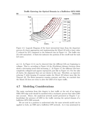
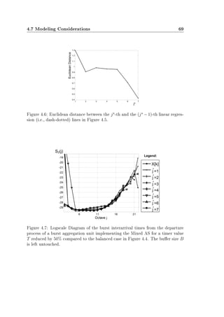


![74 Modeling a Buerless OPS/OBS Network with Poisson Trac
sults with the Erlang Fixed-Point Approximation (EFPA) described in [141, 167].
Section 5.8 introduces some simple model extensions and interesting future lines
of work. One of the model extensions is used in Chapter 7.
5.1 Mathematical Tools
In this section we present some important mathematical tools used in this and
subsequent chapters.
Denition 5.1.1 A nonhomogeneous continuous-time Birth-death (BD) process
{X(t), t ∈ R+
} is a Markov process dened on the set of nonnegative integers N
and with tridiagonal innitesimal generator [139]
q =
q
(0)
1 q
(0)
0
q
(1)
2 q
(1)
1 q
(1)
0
... ... ...
. (5.1)
The term nonhomogeneous refers to the fact that the transition rates {q
(n)
i , i ∈
{0, 1, 2}, n ∈ N} in (5.1) may depend on the level or state n.
According to (5.1), in a BD process only transitions of the form n → n + 1 or
n+1 → n are allowed, for any state n ∈ N. When the BD process is in state n ∈ N,
the time to the next transition of the form n → n + 1 is exponentially distributed
with parameter q
(n)
0 . And if n ∈ N, n ≥ 1, the time to the next transition of the
form n → n−1 is exponentially distributed with parameter q
(n)
2 . The holding time
in state n ∈ N is exponentially distributed with parameter −q
(n)
1 .
In the irreducible case we have that {q
(n)
i 0, i ∈ {0, 2}, n ∈ N} and {q
(n)
1
0, n ∈ N}, and the row sums in q are equal to zero. An irreducible BD process is
ergodic if and only if [105, Theorem 4.5.1]
n≥1
q
(0)
0 · · · q
(n−1)
0
q
(1)
2 · · · q
(n)
2
∞.
In this case its stationary distribution δ = (δ(0), δ(1), . . .) for {X(t), t ∈ R+
}
exists and can be obtained from δq = 0 and δ1 = 1 [139, Corollaries 5.5.4 and
5.5.5]. This yields [144]
δ(n) = δ(0)
n
k=1
q
(k−1)
0
q
(k)
2
, n ≥ 1, (5.2)
where δ(0)−1
= n≥1
n
k=1 q
(k−1)
0 /q
(k)
2 .](https://image.slidesharecdn.com/3f7f65b2-eeec-4afd-a395-b25a5ff55a20-160530113535/85/Modeling_Future_All_Optical_Networks_without_Buff-102-320.jpg)
![5.1 Mathematical Tools 75
In this and subsequent chapters we assume that all BD processes involved are
irreducible and ergodic. Intuitively, this establishes the conditions under which a
Markov process can be analyzed to determine its stationary distribution.
Denition 5.1.2 A continuous-time Markov process {X(t), t ∈ R+
} with state
space E, transition rates q(x, y), x, y ∈ E is reversible if there is a positive measure
δ on E that satises the detailed balance equations [144, Denition 1.4]
δ(x)q(x, y) = δ(y)q(y, x),
with x, y ∈ E.
In an ergodic process the average number of transitions of the process from
state i to state j is equal to the proportion of time δ(i) that the process spends on
state i times the rate at which it makes a transition towards state j [144, Chapter
2]. Thus, for an ergodic process, the equation above can be interpreted as the
equality between the average number of transitions of the process from state x to
state y and in the reverse direction from y to x.
An irreducible ergodic BD process {X(t), t ∈ R+
} with stationary distribution
δ is reversible with invariant measure δ [144, Theorem 2.2].
Independent BD processes can be composed or juxtaposed to form multidimen-
sional BD processes, also called multivariate BD processes [144]. Let × denote the
cartesian product. A formal denition of a multivariate BD follows.
Denition 5.1.3 The juxtaposition X(t) = (X1(t), . . . , XF (t)) of F independent,
irreducible, ergodic BD processes {Xi(t)}1≤i≤F with state spaces {Si}1≤i≤F , dened
on a state space E = S1 × . . . × SF is called a multivariate BD process.
Since the BD processes {Xi(t)}1≤i≤F are irreducible and ergodic, they are also
reversible. Then X(t) = (X1(t), . . . , XF (t)) is an irreducible, ergodic, and re-
versible Markov process with stationary distribution [139, Propositions 2.12 and
2.14] ∆(x), with x = (x1, . . . , xF ) ∈ E,
∆(x) =
1
h
F
i=1
δi(xi), (5.3)
with
h =
x∈E
F
i=1
δi(xi).
A pure birth process {N(t), t ∈ R+
} constitutes a particular case of a BD
process in which {q
(n)
2 = 0, n ∈ N} [105]. Pure birth processes provide simple](https://image.slidesharecdn.com/3f7f65b2-eeec-4afd-a395-b25a5ff55a20-160530113535/85/Modeling_Future_All_Optical_Networks_without_Buff-103-320.jpg)
![76 Modeling a Buerless OPS/OBS Network with Poisson Trac
models of point processes which may describe an ordered set of points (e.g. packet
arrival instants) on [0, ∞). An example of a pure birth process is the Poisson
process introduced in Section 3.3.
Pure birth processes can be generalized to model more complex point processes.
This is the case of Markovian Arrival Processes (MAPs), for which the pure birth
process {N(t), t ∈ R+
} is modulated by a phase process {J(t), t ∈ R+
} whose
state dictates the instantaneous birth rates. A formal denition follows:
Denition 5.1.4 We say that {(N(t), J(t)), t ∈ R+
} is a MAP with representa-
tion MAP(D0, D1) if [105]:
• {(N(t), J(t)), t ∈ R+
} is a bidimensional Markov process dened on N ×
{1, . . . , m}, with m ∈ N nite.
• The corresponding generator is
D0 D1
D0 D1
... ...
. (5.4)
As a consequence of the MAP being Markovian we have that the elements of
D1 and the o diagonal elements of D0 are ≥ 0, the diagonal elements of D0 are
0, and (D0 + D1)1 = 0, where the symbols 0 and 1 represent hereinafter a
column vector of zeros and ones, respectively.
The matrix D0+D1 is the innitesimal generator of the phase process {J(t), t ∈
R+
}. Usually D0 + D1 is irreducible, in which case the stationary distribution ε
associated to the MAP is the unique nonnegative solution of ε(D0 + D1) = 0 and
ε1 = 1. The MAP is stationary if α = ε, where α is the distribution of J(0).
5.2 General Description of the Network Model
We consider a network that operates as follows. The network consists of a nite
number of nodes and each node has a nite number of input and output links.
Packets move among these nodes according to their routing rules. Packets that
follow the same path in the network form what we call a ow. There are F
distinct ows in the network, labeled 1, 2, . . . , F, where F is nite. The physical
interpretation of a ow is a forward equivalent class (FEC) from the MPLS protocol
(see Section 1.4). The network is assumed to be connected. That is, it is not
possible to divide the network in two or more subnetworks such that there are no
packets being transferred from one subnetwork to another.](https://image.slidesharecdn.com/3f7f65b2-eeec-4afd-a395-b25a5ff55a20-160530113535/85/Modeling_Future_All_Optical_Networks_without_Buff-104-320.jpg)
![78 Modeling a Buerless OPS/OBS Network with Poisson Trac
The absence of randomness inside the network permits our model to avoid the
two main assumptions made by other models in the literature such as [46, 45,
173, 5, 141, 167, 163, 159], to cite a few. Namely, the re-sampling of the size (or
transmission time) of a packet and the assumption that the same (e.g., Poisson)
stochastic process describes the arrival of packets at each node in the network.
In particular, in our model the size (or transmission time) of a packet arriving
at the network is random, but it is not re-sampled at each node along its route.
In other words, if the size of a packet is X at the ingress edge node, it is X at
any core node the packet visits, and not an independent random variable with
the same distribution. This takes care of the fact that in an OPS/OBS network
the size of a packet/burst does not change randomly as it travels through the
network. Moreover, our model keeps track of the changes that blocking causes on
the description of the arrival of packets at each link in the network. This models
the interactions taking place between packets in a typical buerless OPS/OBS
network.
After complete observation of the random processes at the entrance of the
network, our network model behaves deterministically. However, it is important
to notice that an observer located at a network link or node with no access to
what happens at the entrance of the network does perceive randomness. For
this reason we call our model a stochastic network model, and we characterize in
Section 5.4 stochastic processes at dierent points inside the network and provide
in Section 5.5 expressions for the blocking probability.
5.3 Model Assumptions
The assumptions we make in this section are quite standard, and also made in the
stochastic network models presented in [129, 29, 104, 103, 46, 45, 173, 5, 141, 167,
159].
Via an ingress link, packets of a given ow i enter the network according to a
Poisson process (see Section 3.3) with intensity λi, with 1 ≤ i ≤ F. The trans-
mission times of packets from ow i are iid (independent, identically distributed)
exponential random variables with parameter µi. Independence is also assumed
between transmission times of packets belonging to dierent ows and between
the transmission times and arrival times of these packets. The packet transmis-
sion time t is a deterministic function of the size s of the packet. In particular,
t = s/c, where c is the channel capacity. As we saw in Section 5.2, packet trans-
mission times are included in the model. However, link propagation times are not
considered, as in [46, 45, 173, 5, 141, 167, 163, 159, 129, 29, 104, 103].](https://image.slidesharecdn.com/3f7f65b2-eeec-4afd-a395-b25a5ff55a20-160530113535/85/Modeling_Future_All_Optical_Networks_without_Buff-106-320.jpg)
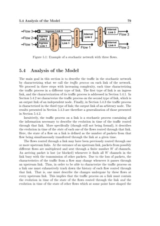
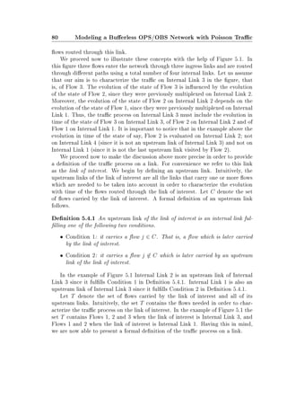
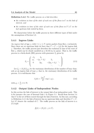
![82 Modeling a Buerless OPS/OBS Network with Poisson Trac
Each component Xj(t), j ∈ C of X(t) represents the state of ow j at time t
on the link of interest. The innitesimal generator of the j-th BD process, j ∈ C
is given by Equation (5.5). The state space E of the trac process is given by
E = {x = (xj : j ∈ C) ∈ N|C|
:
j∈C
xj ≤ W},
where N|C|
denotes the |C|-th cartesian product of N. The state space E includes
all possible ows such that the total number of packets routed through the output
link must be at any time below or equal to the number W of channels in the link.
According to denition 5.1.3 the trac process on any output link of an in-
dependent node is a multivariate BD process. Notice that the multivariate BD
process is constructed by juxtaposing independent BD processes. However, the
components {Xj(t)}j∈C of X(t) do not evolve independently as noticed in Ser-
fozo [144]. The reason for this is the state space E, which introduces a common
restriction on their values. More specically, E implies that j∈C Xj(t) ≤ W for
any time t.
5.4.3 Output Links of Arbitrary Nodes
Let us focus now on the output link of an arbitrary node in the network, which we
call the link of interest. Recall from Section 5.4 that the set T contains the ows
carried by the link of interest and all of its upstream links. Let T(j) denote the
j-th element in T. We dene the constraint matrix A for the link of interest as
follows.
Denition 5.4.3 The constraint matrix A for the link of interest is a L × |T|
matrix with elements Ak,j = 1 if ow T(j) is routed through link k and link k is
either the link of interest or one of its upstream links, and Ak,j = 0 otherwise, for
1 ≤ k ≤ L and 1 ≤ j ≤ |T|.
In Section 5.4.4 we provide algorithms to compute the constraint matrix A and
the sets C and T at the output link of an arbitrary node in the network.
Recalling its denition in Section 5.4, the trac process {X(t), t ∈ R+
} at the
output link (i.e., the link of interest) of an arbitrary node is a |T|-tuple
X(t) = (Xj(t) : j ∈ T),
such that each component Xj(t), j ∈ T represents the following. For j ∈ C, the
component Xj(t) of X(t) represents the state of ow j at time t on the link of
interest. For j ∈ T C, the component Xj(t) of X(t) represents the state of ow
j at time t on the last upstream link visited by this ow.](https://image.slidesharecdn.com/3f7f65b2-eeec-4afd-a395-b25a5ff55a20-160530113535/85/Modeling_Future_All_Optical_Networks_without_Buff-110-320.jpg)
![5.4 Analysis of the Model 83
According to denition 5.1.3 the trac process {X(t)} is a multivariate BD
process subject to the constraint of a restricted state space E(w), given by:
E(w) = {x = (xj : j ∈ T) ∈ N|T|
: Ax ≤ w}, (5.7)
where w is a column vector of dimension L with its k-th component equal to the
number of wavelengths W at the k-th link, 1 ≤ k ≤ L. Some of the rows in
A might be zero. They represent unused links and lead to trivial equations of
the form 0 ≤ W in the system Ax ≤ w. The nontrivial equations in the system
Ax ≤ w represent constraints associated to the link of interest and to each one
of its upstream links. Each constraint imposes that the sum of the number of
packets from the ows in T routed through a given link must be less or equal to
the number of channels W in the link.
From Equation (5.3) we have that the stationary distribution ∆(x) of the trac
process at an arbitrary link is given by
∆(x) =
1
h(w) j∈T
δj(xj), (5.8)
with x ∈ E(w) and where δj(xj) is given by Equation (5.6) and h(w) is a normal-
ization constant, equal to
h(w) =
x∈E(w) j∈T
δj(xj). (5.9)
The transition rates of the trac process are given in Table 5.1 according
to [144, Proposition 2.14], where q(x, y) denotes the transition rate with which
{X(t)} goes from state x to state y. This table is built by considering every
possible transition of X(t) within its state space E (second column of the table),
and by observing the rate at which X(t) performs such a transition (rst column
of the table).
Value q(x, y) Condition
λj y = x + ej, x ∈ E(w − Aej)
xjµj y = x − ej
− j∈T [q(x, x + ej)+ y = x
q(x, x − ej)]
0 otherwise
Table 5.1: Transition rates of the trac process {X(t)}, for j ∈ T.
In Table 5.1, ej denotes a vector of zeros with the value one at position j. Note
that the condition x ∈ E(w − Aej) in this table is to ensure that the transition](https://image.slidesharecdn.com/3f7f65b2-eeec-4afd-a395-b25a5ff55a20-160530113535/85/Modeling_Future_All_Optical_Networks_without_Buff-111-320.jpg)
![84 Modeling a Buerless OPS/OBS Network with Poisson Trac
x → x + ej takes place within the state space E(w) of the trac process, that is,
A(x + ej) ≤ w.
The trac process at an arbitrary link is the same type of constrained multi-
variate BD process arising in the analysis of stochastic networks modeling circuit-
switching networks (see for instance [129, 29, 144] and references therein). The
main dierence here is that in circuit-switched models there is one multivariate
BD process to describe the whole network, while in our case we have a dierent
one for each internal link in the network. Every multivariate BD process has its
own constraint matrix A, sets C and T, and product-form solution given by Equa-
tion (5.8). In the following section we show how to compute A, C and T at every
internal link in the network.
5.4.4 Algorithms for the Constraint Matrix A and the Sets
T and C
In this section we provide two algorithms. The rst one computes the constraint
matrix A, and also provides the set T. The second computes set C of ows routed
through the link of interest.
The starting point for the computation of A, T and C is the routing table R of
the network. The routing table is a collection of F vectors {R1, . . . , RF }, where
the k-th entry Rj(k) is the index of the k-th link in the ordered sequence of links
dening the path of the j-th ow. The indices of the ingress links are not included
in R. Routing tables might appear in the literature as the ordered sequence of
nodes visited by a ow (see for instance [118]). The conversion from this node-
oriented to our link-oriented routing table is immediate. An example of a routing
table can be found in Table 5.2.
Both algorithms make use of a function Find (i,V), which takes a value i and
a vector V as input and provides the index j such that V (j) = i. If the value i is
not found in V , the function returns the value −1.
Algorithm 1 returns the matrix of constraints A and the set T for a given link
of interest indexed by i, with 1 ≤ i ≤ L. The algorithm is recursive and must be
invoked the rst time with the index i of the link of interest, a L × F matrix Z of
zeros, and the routing table R.
A brief explanation for the way Algorithm 1 works follows. In the rst call to
the algorithm ComputeAandT (i, Z,R), i is the index of the link of interest. The
algorithm then calls itself recursively with the index i of every upstream link of
the link of interest. In each call, the algorithm ComputeAandT (i, Z,R) writes the
constraints in the matrix Z corresponding to the ows being carried by the link
indexed by i. Thus, when all recursions are nished Z contains the constraints
corresponding to the ows being carried through the link of interest and through](https://image.slidesharecdn.com/3f7f65b2-eeec-4afd-a395-b25a5ff55a20-160530113535/85/Modeling_Future_All_Optical_Networks_without_Buff-112-320.jpg)
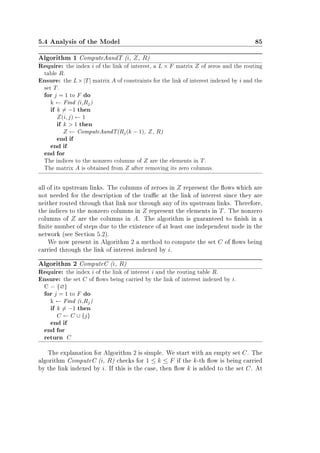
![86 Modeling a Buerless OPS/OBS Network with Poisson Trac
the end of the for statement all ows carried by the link with index i have been
written in C.
5.5 Blocking Probability
In this section we compute the blocking probability in three dierent cases. The
rst case, developed in Section 5.5.1, concerns the blocking probability at any given
link for any packet of a particular ow. The second case, developed in Section 5.5.2,
refers to the blocking probability any given link for any packet of any of the ows
routed through that link. The third case, addressed in Section 5.5.3, concerns the
blocking probability for any packet of a particular ow at any link throughout the
end-to-end path of the ow.
In order to be able to distinguish among dierent links in the network we
add a subindex k to the notation introduced in Section 5.4 to make an explicit
reference to the link k under study, 1 ≤ k ≤ L. The trac process on link k
is now written as {Xk(t) = (Xj,k(t) : j ∈ Tk), and it is dened on Ek(w) =
{x = (xj : j ∈ Tk) ∈ N|Tk|
: Akx ≤ w}, where w is a vector of length L. Its
stationary distribution is given by ∆k(x) = 1
hk(w) j∈Tk
δj(xj), where x ∈ Ek(w)
and hk(w) = x∈Ek(w) j∈Tk
δj(xj).
Let Nj,k(t) denote the number of packets from ow j arriving at link k during
(0, t], j ∈ Ck, 1 ≤ k ≤ L, t ∈ R+
.
Denition 5.5.1 The average arrival rate rj,k of packets from ow j at link k is
equal to the time average rj,k(t) = t−1
Nj,k(t), when t → ∞.
Before addressing the computation of the blocking probabilities in each one
of the three cases mentioned above, we introduce the following proposition which
permits us to compute the average arrival rate of packets from ow j at link k.
Proposition 5.5.2 The average arrival rate of packets from ow j, j ∈ Ck at link
k converges w.p. 1 to the constant
rj,k = λj
hk(w − Akej)
hk(w)
, (5.10)
where ej denotes a vector of zeros with the value one at position j.
Proof: Let |G| denote the cardinal of the set G. We consider a bijective function
g : Ek(w) → {1, . . . , |Ek(w)|} which univocally assigns a dierent nonnegative
integer to each vector x ∈ Ek(w), and let us denote by g−1
its inverse.
Consider the bidimensional Markov process {Nj,k(t), J(t)} taking values on
N × {1, . . . , |Ek(w)|} with a block-bidiagonal generator of the form given in (5.4)](https://image.slidesharecdn.com/3f7f65b2-eeec-4afd-a395-b25a5ff55a20-160530113535/85/Modeling_Future_All_Optical_Networks_without_Buff-114-320.jpg)
![5.5 Blocking Probability 87
with matrices D0 and D1 behaving as follows. Every time that the trac process
{Xk(t)} on link k makes a transition, the MAP(D0, D1) registers that transition in
D0 as a change of phase. There is one exception to this rule, which takes place when
the transition of {Xk(t)} is of the form x → x + ei, with x ∈ Ek(w − Akei). This
transition represents an arrival of a packet from ow i at link k that is not blocked
by the system, where non blocking is ensured by condition x ∈ Ek(w−Akei). In this
case the MAP(D0, D1) registers that transition in matrix D1 as a packet arrival,
instead of as a phase transition in matrix D0. We now characterize the matrices
D0 and D1 of the MAP(D0, D1) according to this description. For 1 ≤ nx, ny ≤
|Ek(w)|, let x = g−1
(nx) and y = g−1
(ny). Then, the o-diagonal elements in D0
are given by:
D0(nx, ny) =
λi if y = x + ei, x ∈ Ek(w − Akei), i = j
xiµi if y = x − ei
0 Otherwise
(5.11)
The elements in D1 are given by D1(nx, ny) = λj if y = x + ej and x ∈
Ek(w − Akej), and zero otherwise, and the elements in the diagonal of D0 are so
that the row sums of (D0 + D1) are equal to zero.
According to the denition above this process is a MAP (Markovian Arrival
Process, see [105]), for which Nj,k(t) is the number of arrivals in (0, t] and J(t) is
the phase at time t. Since D0 + D1 is irreducible, the stationary distribution ε
of this MAP is given by the unique nonnegative solution of ε(D0 + D1) = 0 and
ε1 = 1. Its mean density mj,k = E[Nj,k(1)] is given by [105]:
mj,k = εD11, (5.12)
where 1 is a column vector of ones.
Notice from Equation (5.11) and the denition of D1 that q(g−1
(nx), g−1
(ny)) =
D0(nx, ny) + D1(nx, ny), where q(x, y) denotes the transition rates of the trac
process {Xk(t)} on link k given in Table 5.1. That is, under a bijective trans-
formation g the transition rates of the trac process {Xk(t)} at link k are equal
to the transition rates of the phase process {J(t)} in the MAP. This implies that
under the same transformation, the stationary distribution ∆k of {Xk(t)} is equal
to the stationary distribution ε of the MAP. That is, ε(m) = ∆k(g−1
(m)), for
1 ≤ m ≤ |Ek(w)|. Substituting ε(m) by ∆k(g−1
(m)) in Equation (5.12) yields:
mj,k = λj
x∈Ek(w−Akej)
∆k(x), (5.13)
which is equal to the right-hand side in Equation (5.10). Moreover, since the MAP
(Nj,k(t), J(t)) has a nite number of phases, it is an ergodic process [139]. Thus,
we have that the time average rj,k(t) = t−1
Nj,k(t) converges w.p. 1 to mj,k when](https://image.slidesharecdn.com/3f7f65b2-eeec-4afd-a395-b25a5ff55a20-160530113535/85/Modeling_Future_All_Optical_Networks_without_Buff-115-320.jpg)
![88 Modeling a Buerless OPS/OBS Network with Poisson Trac
Figure 5.2: Blocking probability βj,O for ow j at the output link O of an arbitrary
node. Output link O carries packets from ow j and possibly from other ows.
Packets from ow j enter the node through input link I.
t → ∞ [36]. Thus, the left-hand side in Equation (5.13) is equal to rj,k(t), which
concludes the proof.
Note that in our stochastic network model the average arrival rate rj,k of packets
from ow j depends on the link k, since any packet may be blocked at each link
it visits.
5.5.1 Blocking of a Flow at a Node
Let us begin with the rst case and consider ow j for some given j on the output
link of an arbitrary node like the one in Figure 5.2, which we denote output link
O. Assume that ow j arrives at the node through input link I (see Figure 5.2).
We want to compute the stationary probability that an arriving packet from ow
j nds all W channels at the output link O busy with the transmission of other
packets. We shall refer to this as the packet blocking probability βj,O.
Let {tn}n≥0 be the increasing sequence of arrival times of the packets from ow
j at link k. We dene {Zj,k[n], n ∈ N} as:
Zj,k[n] = Xk(tn). (5.14)
That is, {Zj,k[n], n ∈ N} represents the trac process on link k observed at the
arrival times of the packets from ow j at this link. We introduce the following
proposition, which will be used to derive βj,O.
Proposition 5.5.3 The stochastic process {Zj,k[n], n ∈ N}, j ∈ Ck, 1 ≤ k ≤ L
dened in Equation (5.14) is a stationary Markov chain.](https://image.slidesharecdn.com/3f7f65b2-eeec-4afd-a395-b25a5ff55a20-160530113535/85/Modeling_Future_All_Optical_Networks_without_Buff-116-320.jpg)
![5.5 Blocking Probability 89
Proof Let {Xk[n], n ∈ N} be the embedded discrete-time Markov chain of {Xk(t), t ∈
R+
}. That is, {Xk[n]} is obtained after sampling {Xk(t)} at its transition times
{τn}n≥0 (i.e., Xk[n] = Xk(τn)). Let us denote by {un}n≥0 the increasing sequence
of indices at which {Xk[n]} makes a transition of the form x → x + ej. This
sequence is dened for n ≥ 0 as:
un = inf{m ∈ N : Xk[m] = Xk[m − 1] + ej, m un−1},
where u−1 = −1.
From this denition it is clear that {Zj,k[n]} can be also expressed as:
Zj,k[n] = Xk[un], (5.15)
with n ≥ 0.
The instants {un}n≥0 can be easily veried to be stopping times for the Markov
chain {Xk[n]}, since the event {un = m} depends only on Xk[0], . . . , Xk[m]. Thus,
the strong Markov property implies that {Zj,k[n]} is a Markov chain [15].
The stationarity of {Xj,k(t)} implies that of its embedded discrete-time Markov
chain {Xk[n]} [139]. From this and Equation (5.15), the stationarity of {Zj,k[n]}
immediately follows.
We present now the main result from this section.
Proposition 5.5.4 The packet blocking probability βj,O for ow j on link O is
given by:
βj,O = 1 −
rj,O
rj,I
, (5.16)
where rj,O and rj,I are the average arrival rates of packets from ow j at links O
and I, respectively and are given by (5.10).
Proof: From Proposition 5.5.3 we have that {Zj,k[n]} is a stationary Markov chain.
Let γj,k(·) be its stationary distribution. The stationarity of {Zj,O[n], n ∈ N}
allows us to apply the ergodic theorem for discrete-time Markov chains (see [139,
Proposition 2.12.4]), which states that:
lim
N→∞
N−1
N
n=0
f(Zj,O[n]) =
x∈EO(w)
f(x)γj,O(x), (5.17)
for a suitable function f : EO(w) → R. Let us dene f as
f(x) = 1EO(w−AOej)(x),](https://image.slidesharecdn.com/3f7f65b2-eeec-4afd-a395-b25a5ff55a20-160530113535/85/Modeling_Future_All_Optical_Networks_without_Buff-117-320.jpg)
![90 Modeling a Buerless OPS/OBS Network with Poisson Trac
where 1A(x) is the indicator function, equal to 1 if x ∈ A and equal to 0
otherwise. The left-hand side of Equation (5.17) denotes the fraction of arriving
packets from ow j which nd an available channel at link O. This fraction is
equal to limt→∞ Nj,O(t)/Nj,I(t), where Nj,k(t), k = {O, I} denotes the number of
packets from ow j arriving at link k during (0, t]. Since Nj,k(t), k = {O, I} is the
number of arrivals in (0, t] of an ergodic MAP (see the proof of Proposition 5.5.2),
dividing both the numerator and denominator by t leads to the conclusion that
the left-hand side of Equation (5.17) is equal to rj,O/rj,I.
The right-hand side of Equation (5.17) is equal to
x∈EO(w−AOej)
γj,O(x).
We now relate this equation to the packet blocking probability βj,O for ow j
on link O. According to its denition in Section 5.5.1, βj,O can be expressed as the
complement of the probability that an arriving packet from ow j is not blocked
in the link. That is:
βj,O ≡ 1 − lim
n→∞
P[Zj,O[n] ∈ EO(w − AOej)],
where the second term in the right-hand side is the stationary probability that an
arriving packet from ow j nds at least one available channel for its transmission
over link O. From the stationarity of {Zj,k[n]} it follows (see [139, Proposition
2.13.1]) that
βj,O = 1 −
x∈EO(w−AOej)
γj,O(x), (5.18)
and thus the right-hand side of Equation (5.17) is equal to 1−βj,O, which concludes
the proof.
5.5.2 Blocking at the Output Link of a Node
Let us address now the second case mentioned at the beginning of this section.
Consider again Figure 5.2. We wish now to compute the stationary probability
βO that a packet from any of the ows routed through output link O nds upon
arrival at this link all its W channels busy with the transmission of other packets.
We shall refer to this as the packet blocking probability βO at link O.
Proposition 5.5.5 The packet blocking probability βO at the output link O of an
arbitrary node is given by](https://image.slidesharecdn.com/3f7f65b2-eeec-4afd-a395-b25a5ff55a20-160530113535/85/Modeling_Future_All_Optical_Networks_without_Buff-118-320.jpg)
![5.5 Blocking Probability 91
βO = 1 −
j∈CO
rj,O
k∈I j∈Ck∩CO
rj,k
, (5.19)
where I is the set of input links to the node carrying at least one ow in CO, and
where rj,O and rj,k are given by Equation (5.10).
Proof: Let {tn}n≥0 be the increasing sequence of arrival times of the packets from
the ows routed through link k (i.e., the ows in Ck). We dene {Zk[n], n ∈ N} as
Zk[n] = Xk(tn). This process represents the trac process on link k observed at
the arrival times of the packets of the ows routed through this link. Following the
same arguments as in the proof of Proposition 5.5.3 we conclude that {Zk[n], n ∈
N} is a stationary Markov chain with stationary distribution γk
.
The packet blocking probability βO at link O can be expressed as βO =
P[∩1≤i≤Omax Vi], where Vi denotes the event {an arriving packet from ow i nds
all W channels on link O busy}. We also have that β = 1−P[∪1≤i≤Omax Si], where
Si denotes the event {an arriving packet from ow i nds at least one channel on
link O available}. That is, βO ≡ 1 − limt→∞ P[ZO[n] ∈ DO], where
DO = ∪j∈CO
EO(w − AOej).
The set DO represents the following. When the trac process XO(t) at link
O is in any of the states that belongs to DO, the link has at least an available
channel for the arrival of a packet from any of the sources in CO routed through
it.
Thus,
βO = 1 −
x∈DO
γO(x).
We now follow the same arguments as in the proof of Proposition 5.5.4 and
apply the ergodic theorem to {Zk[n]} using the function
f(x) = 1DO
(x).
This leads to βO = 1 − rO/rI, where rO denotes the sum of the average arrival
rate of packets from the ows on link O and rI represents sum of the average
arrival rate of packets from each one of the ows in CO measured on its corre-
sponding input link at the node. Equation (5.19) immediately follows from the
use of Proposition 5.5.2.](https://image.slidesharecdn.com/3f7f65b2-eeec-4afd-a395-b25a5ff55a20-160530113535/85/Modeling_Future_All_Optical_Networks_without_Buff-119-320.jpg)
![92 Modeling a Buerless OPS/OBS Network with Poisson Trac
5.5.3 Blocking of a Flow
We proceed now with the third case mentioned at the beginning of this section.
We want to provide an expression for the stationary probability that a packet
from ow j arriving at the network, 1 ≤ j ≤ F nds all W channels busy at one
of the links in its end-to-end route. We shall refer to this as the packet blocking
probability βj for ow j.
Recall from Section 5.4.4 that Rj(k) denotes the k-th link visited in the routing
table entry Rj for the j-th ow, with 1 ≤ j ≤ F, 1 ≤ k ≤ jmax, and jmax is the
length Rj. Consider the sequence of successive state spaces {ERj(1), . . . , ERj(jmax)}
of the trac process at each one of the links along the route of ow j. Each
system ARj(k+1)x ≤ w has the same equations as ARj(k)x ≤ w plus some additional
inequalities (see the denition of the constraint matrix A in Denition 5.4.3),
1 ≤ k ≤ jmax − 1. Thus, we have
ERj(jmax) ⊆ ERj(jmax−1) ⊆ · · · ⊆ ERj(1).
This suggests that in order to check if a packet from ow j is not blocked at
any of the links from its path it suces to check that it is not blocked at the last
link in the path jmax, which for convenience we rename now as link O. With this
in mind we can rephrase the packet blocking probability βj for ow j as one minus
the probability that a packet from ow j arriving at the network nds an available
channel at the last link O in its end-to-end route. In what follows we call the
egress link of ow j to the last link O in its end-to-end route.
Proposition 5.5.6 The packet blocking probability βj for ow j, 1 ≤ j ≤ F is
given by
βj = 1 −
hO(w − AOej)
hO(w)
, (5.20)
where O, 1 ≤ O ≤ F is the egress link of ow j in the network.
Proof: Let {tn}n≥0 be the increasing sequence of arrival times of the packets from
ow j at the network, that is, at its ingress link I. We dene {ZO[n], n ∈ N}
as ZO[n] = XO(tn). This process represents the trac process on the egress
link O of ow j observed at the arrival times of the packets ow j at its ingress
link I. Following the same arguments as in the proof of Proposition 5.5.3 and
Proposition 5.5.4 we conclude that βj = 1 − rj,O/rj,I, where rj,I is the average
arrival rate of packets from ow j at the network (i.e., at its ingress link I). This
is equal to its Poisson intensity λj. Taking this into account and expanding rj,O
from Equation (5.10) concludes the proof.](https://image.slidesharecdn.com/3f7f65b2-eeec-4afd-a395-b25a5ff55a20-160530113535/85/Modeling_Future_All_Optical_Networks_without_Buff-120-320.jpg)
![5.6 Computational Issues 93
We conclude this section with a short remark. Let us dene the time blocking
probability αj for ow j as the stationary probability that all W channels at the
egress link O of ow j are busy with the transmission of packets. Since the arrival
process of ow j is Poisson, from the PASTA property (see [170]) we have that αj =
βj. This result can be observed in Equation (5.20) by noticing that βj represents
1 − P[at least one channel in O is available], which is equal to αj. However, in
our model the input trac at an arbitrary node is in general not Poisson, since
blocking might have taken place at some upstream nodes. Therefore, the PASTA
property does not apply to Propositions 5.5.4 and 5.5.5, where the packet blocking
probabilities are generally not equivalent to their corresponding time blocking
probability denitions.
5.6 Computational Issues
The computation of the blocking probability requires the evaluation of hk(b) for
some nonnegative integer vector b and link k, 1 ≤ k ≤ N (see Equations (5.16), (5.20)
and (5.19)). This involves the computation of the sum of a function ∆k(x) evalu-
ated at every point x inside the convex polytope {x ∈ N|Tk|
: Akx ≤ b}.
The evaluation of hk(b) is not a problem specic to our model. In fact, hk(b)
is the well-known partition function which has been studied over the last two
decades in order to compute the blocking probability in many models of circuit-
switching networks [144, 129, 29, 104, 103]. Thus, although our model is new,
its computational aspects rely on solid theoretical foundations. We now briey
summarize the main methods presented in the literature to compute the partition
function hk(b).
In [109] it was demonstrated that the exact computation of hk(b) is a P-
complete problem. According to current common notions in complexity theory,
it is believed that the class of P-complete problems is intractable, as dened
in [64]. In fact, state-of-the-art exact algorithms such as [129, 29], cannot solve
hk(b) in polynomial time. Unless further simplifying assumptions are made, their
complexity remains O(F · WL
), where F is the number of ows, W is the number
of channels per link and L is the number of links.
In optical networks the number of wavelength channels W per optical ber
can be rather high (e.g. W = 80 or W = 160), which makes the evaluation of
hk(b) using the above mentioned methods impractical in many realistic network
congurations. In this case the use of Monte Carlo (MC) simulation techniques in
order to estimate the value of hk(b) is recommended. In [104, 103] and references
therein several MC methods have been devised for this purpose. The main idea is
to interpret the partition function hk(b) as the expectation of a function Ψ(Z) of
a discrete random variable Z distributed according to ∆k, with Ψ(x) = 1Ek(b)(x),](https://image.slidesharecdn.com/3f7f65b2-eeec-4afd-a395-b25a5ff55a20-160530113535/85/Modeling_Future_All_Optical_Networks_without_Buff-121-320.jpg)
![94 Modeling a Buerless OPS/OBS Network with Poisson Trac
Figure 5.3: NSFNET backbone network
and where Ek(b) is given by Equation (5.7). That is, hk(b) = E[Ψ(Z)]. The main
advantage of the MC method is that its error is O(δ/n1/2
), where n is the number
of iterations and δ is the standard deviation of Ψ(Z) [62]. Notably, this error is
independent of F, W and L, which makes it a viable solution when W is large.
In order to make the MC simulation more ecient, it is possible to employ a
technique called Importance Sampling (IS). With IS one uses an alternative sam-
pling distribution ∆ which reduces the standard deviation δ of Ψ(Z), reducing
the error O(δ /n1/2
) of the MC simulation. Importance sampling has proven to be
particularly useful for the evaluation of the partition function [104, 103].
5.7 Numerical Study
In this section the stochastic network presented in this chapter is used in order
to model the network topology depicted in Figure 5.3 (see [141] and references
therein). The main objective is twofold. First, we want to have a quantitative
idea of the approximation error of the Erlang Fixed-Point Approximation (EFPA)
method compared to our model. The EFPA is a de facto standard model for the
computation of the blocking probability in buerless packet switching networks.
It is simple and elegant, but it is also uses important simplifying assumptions. For
this reason we want to nd out if the predictions from the EFPA substantially
dier from the predictions of our model. Second, we want to show that our model
is analytically tractable by computing with it blocking probabilities in a realistic
network conguration.
The topology of the network in Figure 5.3 corresponds to the National Science](https://image.slidesharecdn.com/3f7f65b2-eeec-4afd-a395-b25a5ff55a20-160530113535/85/Modeling_Future_All_Optical_Networks_without_Buff-122-320.jpg)
![5.7 Numerical Study 95
Foundation NETwork (NSFNET), which connects a large number of industry and
academic campuses across the USA. The network comprises 13 OPS/OBS switches
and L = 30 unidirectional bre links, each one comprising W wavelength channels
at 10 Gbps each. Table 5.2 presents the dierent trac routes considered in the
network for a total number of F = 12 ows. In this table, Ri, 1 ≤ i ≤ 12
represents the ordered sequence of nodes visited by packets from the i-th ow.
As it was mentioned in Section 5.4.4 it is straightforward to transform this table
into the routing table needed by the algorithms in Section 5.4.4. The routes in
Table 5.2 represent a variety of path lengths, link sharing degrees and mixtures
of external and on-route internal trac processes. All routes are shortest paths,
except for R3 and R7 that are selected to obtain better route diversity.
Route Name Nodes Visited
R1 1 → 4 → 6 → 5 → 8 → 10
R2 2 → 3 → 5 → 6 → 7
R3 2 → 7 → 9 → 12 → 13
R4 3 → 5 → 8 → 13
R5 5 → 6 → 7 → 9 → 12
R6 8 → 10 → 11 → 12 → 13
R7 10 → 8 → 5 → 6 → 4 → 1
R8 7 → 6 → 5 → 3 → 2
R9 13 → 12 → 9 → 7 → 2
R10 13 → 8 → 5 → 3
R11 12 → 9 → 7 → 6 → 5
R12 13 → 12 → 11 → 10 → 8
Table 5.2: NSFNET routes
In what follows we refer simply by blocking probability to the packet blocking
probability dened in Section 5.5. We have used three dierent methods in order
to compute the blocking probabilities in the NSFNET backbone network. The rst
two methods constitute two dierent computational approaches for our network
model. The third method is approximative.
The rst method uses the so-called Normalization Constant Approach pre-
sented in [129]. This makes use of a recursive algorithm to compute the exact
value of the partition function hk(w). For this reason, in what follows we refer to
this method as the Exact solution.
The second method uses Monte Carlo simulations with importance sampling
techniques, as described in [103]. In order to estimate each partition function
hk(w), 500 simulations were used, each one with n = 15000 samples. Due to the
high number of simulations the 95%-condence intervals are too small to be seen](https://image.slidesharecdn.com/3f7f65b2-eeec-4afd-a395-b25a5ff55a20-160530113535/85/Modeling_Future_All_Optical_Networks_without_Buff-123-320.jpg)
![96 Modeling a Buerless OPS/OBS Network with Poisson Trac
Figure 5.4: Blocking probability βj for all ows 1 ≤ j ≤ 12 in the network for load
vector ρ = (2, 1.3333, 1, 0.7667, 0.8, 0.7843, 0.8, 0.2, 1.6, 2, 0.16, 1.2).
in the gures. For this reason they have been removed. In what follows we refer
to this method as the MC solution.
The third method uses the EFPA described in [141] to compute the link and
ow blocking probabilities. In what follows we refer to this method as the EFPA
solution. In the EFPA model packets are assumed to arrive at each node in the
network according to a Poisson process. That is to say, the packet arrival process is
re-sampled at each node in the network. Moreover, packet transmission times (and
therefore packet sizes) are assumed to be re-sampled at each node in the network
from an exponential distribution. Re-sampling of these two stochastic processes
(sometimes referred to as link blocking independence [163]) inevitably implies the
loss of information concerning the blocking events of packets along the routes in
the network, which makes the description of trac in the EFPA model incomplete.
Let us dene the average load vector as ρ = (λ1/µ1, . . . , λ12/µ12), where λi and
1/µi represent the average packet arrival time and the average burst transmission
time for packets in ow i, respectively.
Figures 5.4 and 5.5 present the ow blocking probability for each one of the
12 ows in the network and for two dierent values of the average load vector.](https://image.slidesharecdn.com/3f7f65b2-eeec-4afd-a395-b25a5ff55a20-160530113535/85/Modeling_Future_All_Optical_Networks_without_Buff-124-320.jpg)
![5.7 Numerical Study 97
Figure 5.5: Blocking probability βj for all ows 1 ≤ j ≤ 12 in the network for load
vector ρ = (2, 0.1333, 2, 0.1, 1.3333, 0.0157, 0.8, 0.02, 0.16, 2, 0.16, 2).
In both cases the ow blocking probability is computed with the Exact solution,
the EFPA method and using the Monte Carlo estimator from [103]. We work
with W = 8 wavelength channels per link in order to be able to use the Exact
solution presented in [129]. Due to its complexity of O(F · WL
) (see Section 5.6),
for W 8 this solution becomes impractical for the network under study. The
purpose of using the Exact solution in this gure is to be able to double-check the
Monte Carlo simulation.
From Figures 5.4 and 5.5 we can conclude that the Monte Carlo method pro-
vides a very accurate estimation of the exact blocking probability. We can also
observe that for some routes the EFPA provides fairly good approximations of the
blocking probabilities (e.g., routes 4 and 12 in Figure 5.4 and routes 9 and 11 in
Figure 5.5), while for others not (e.g., routes 1 and 10 in Figure 5.4 and routes 3
and 5 in Figure 5.5).
The worst case in Figures 5.4 and 5.5 constitutes the approximation of the
blocking probability for route 1 with the EFPA, which leads to percentage errors
around 75% and 500%, respectively. We now focus on route 1 and proceed to pro-
vide some insight into the reason why such nonnegligible dierences exist between](https://image.slidesharecdn.com/3f7f65b2-eeec-4afd-a395-b25a5ff55a20-160530113535/85/Modeling_Future_All_Optical_Networks_without_Buff-125-320.jpg)
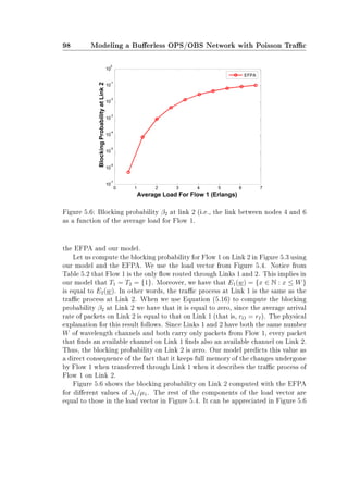
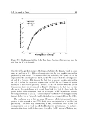
![100 Modeling a Buerless OPS/OBS Network with Poisson Trac
Figure 5.8: Blocking probability β1 for ow 1 as a function of the average load for
this ow for W = 160 channels.
ally increases the blocking probability [140]. However, adding realism means in our
case making the model more deterministic (i.e., no randomness inside the network
is allowed), and less randomness usually improves performance.
We proceed now to study the scalability of our model. Figure 5.7 presents
the blocking probability for Flow 3 as a function of the average load for this ow,
dened as λ3/µ3. The average load of the rest of the ows in the network was
changed proportionally to that of ow 3 with respect to the average load vector
used in Figure 5.4. The number of wavelength channels per link is W = 8.
Figure 5.8 presents the blocking probability for Flow 1 as a function of the
average load for this ow, dened as λ1/µ1. The average load of the rest of the
ows in the network was changed proportionally to that of ow 1 with respect
to the average load vector used in Figure 5.5. The main dierence compared to
Figure 5.7 is that we use a number of W = 160 wavelength channels per link.
This value of W corresponds to a more realistic OBS/OPS scenario than the
previous one and makes the exact computation of the blocking probability with
the Normalization Constant Approach presented in [129] unpractical.
As Figure 5.8 illustrates, it is still viable to use Monte Carlo simulations in
order to compute the blocking probability in a scenario with W = 160 wavelength](https://image.slidesharecdn.com/3f7f65b2-eeec-4afd-a395-b25a5ff55a20-160530113535/85/Modeling_Future_All_Optical_Networks_without_Buff-128-320.jpg)
![5.8 Model Extensions and Future Work 101
channels per link (i.e., 160 servers per node). This indicates that the analytical
model presented in this paper is scalable within reasonable limits. In particular,
the Monte Carlo simulation method with importance sampling presented in [103]
provided an estimation of each blocking probability in Figure 5.7 in about 25
seconds in an Intel CoreTM processor with 2GB of RAM. Each estimation in
Figure 5.8 was computed in about the same time in the same computer. This
clearly illustrates the fact that the complexity of the Monte Carlo simulation does
not scale with W, as it does in the exact methods presented in [129].
Finally, we can observe in Figure 5.7 that once more the Monte Carlo method
provides an excellent estimation of the exact blocking probability (both curves are
superposed), while the EFPA method leads to nonnegligible approximation errors.
In particular, the percentage error in this gure oscillates between 55% and 75% for
the EFPA, while for the Monte Carlo simulation it remains below 2%. Regarding
Figure 5.8, the relative error between the EFPA and the MC approaches in this
case oscillates between 30% and 80%. This indicates that even with W = 160
wavelength channels per link the use of full memory in our model accounts for
nonnegligible dierences compared to the EFPA.
5.8 Model Extensions and Future Work
It is possible to generalize the trac process on an ingress link in Section 5.4.1
to a nonhomogeneous BD process with generator given in Equation (5.1). One
possible use of this is to be able to make the Poisson arrival rates and exponential
service times depend on the channel occupation level at the ingress links.
In Chapter 7 we make a dierent use of this generalization; we use it to solve
under certain assumptions the more complex case in which the packet arrival
process for every ow is a MAP and packet transmission times are Markovian. For
this reason we provide now more details on this generalization and refer to them
in Chapter 7.
Let us assume that the trac process on an ingress link j is a nonhomogeneous
irreducible ergodic BD process with generator qj, 1 ≤ j ≤ F given by Equa-
tion (5.1). We add a subindex j to the notation in Equation (5.1) in order to
dierentiate among dierent ingress links. That is, the rates of BD process j are
written as {q
(n,j)
i , i ∈ {0, 1, 2}, n ≥ 0, 1 ≤ j ≤ F}. Then the trac process on
the output link k, 1 ≤ k ≤ L of an arbitrary node is a multivariate BD process
with stationary distribution ∆k given by Equation (5.8), with δj being the unique
nonnegative solution of δjqj = 0 and δj1 = 1 [139, Theorem 5.5.4], j ∈ Tk. Then
we have the following result.](https://image.slidesharecdn.com/3f7f65b2-eeec-4afd-a395-b25a5ff55a20-160530113535/85/Modeling_Future_All_Optical_Networks_without_Buff-129-320.jpg)
![102 Modeling a Buerless OPS/OBS Network with Poisson Trac
Proposition 5.8.1 The average arrival rate of packets from ow j, j ∈ Ck at link
k converges w.p. 1 to the constant
rj,k =
1
hk(w)
x∈Ek(w−Akej) m∈Tk
δm(xm)q
(xj,j)
0 . (5.21)
Proof: The proof is analogous to that of Proposition 5.5.2 except for the following
dierences.
The o-diagonal elements in D0 are now given by:
D0(nx, ny) =
q
(xi,i)
0 if y = x + ei, x ∈ Ek(w − Akei), i = j
q
(xi,i)
2 if y = x − ei
0 Otherwise
The elements in D1 are given by D1(nx, ny) = q
(xj,j)
0 if y = x + ej and x ∈
Ek(w − Akej), and zero otherwise, and the elements in the diagonal of D0 are so
that the row sums of (D0 + D1) are equal to zero.
According to this, the mean density mj,k = E[Nj,k(1)] of the MAP is equal
to the right-hand side in Equation (5.21). From the ergodicity of the MAP we
have that the time average rj,k(t) = t−1
Nj,k(t) converges w.p. 1 to mj,k when
t → ∞ [36], which concludes the proof.
The expressions for the packet blocking probabilities in Sections 5.5.1 and 5.5.2
remain unchanged. The one in Section 5.5.3 cannot be simplied now to the extent
of Equation (5.20). Following the proof of Proposition 5.5.6 this expression can be
now easily seen to be equal to
βj = 1 − rj,O/rj,I,
where rj,I is the average arrival rate of packets from ow j at the network (i.e., at
its ingress link I), and rj,k(t) is given by Equation (5.21), 1 ≤ j ≤ F, 1 ≤ k ≤ L.
Some other extensions of the model are immediate. For instance, it is possible
to use a dierent number of channels Wk in each link 1 ≤ k ≤ L of the network.
This may model transmission links with dierent number of deployed bers, or
bers with dierent number of wavelength channels.
It is also possible that the elements of the constraint matrices Ak, 1 ≤ k ≤ L
take values in N. That is, that a ow j may use more than one channel at link
i simultaneously. This feature might be interesting for modeling trac groom-
ing [183] in OPS/OBS networks, where ows may arrive at the network through
links with dierent capacities. We now briey introduce this case. Consider a
network of F ows, where each ow j, 1 ≤ j ≤ F has an associated granularity
G(j) that represents its grooming level. Moreover, let the transmission channel
capacity c in our model represent the capacity of the nest grooming granularity,](https://image.slidesharecdn.com/3f7f65b2-eeec-4afd-a395-b25a5ff55a20-160530113535/85/Modeling_Future_All_Optical_Networks_without_Buff-130-320.jpg)
![5.8 Model Extensions and Future Work 103
that is, with G(j) = 1. For instance, a ow j with granularity G(j) could demand
for a capacity equivalent to that of the SONET Optical Carrier Level OC − G(j),
and c could be the capacity of SONET Optical Carrier Level OC-1 (51.84 Mbps).
With this scenario, Algorithm 1 can be used to compute the constraint matrix A
for a given link of interest after using the statement
A(i, j) ← G(j),
instead of A(i, j) ← 1. This statement simply acknowledges the fact that a ow
with granularity G(j) demands in each link for G(j) times the capacity of the
basic transmission channel of capacity c. In our example, an OC − 3 ow j (that
is, G(j) = 3) requires three times the capacity c of an OC − 1 ow. The rest
of the algorithms and equations in this work apply without modications to this
grooming case.
The similitude between the proposed model and other stochastic network mod-
els for circuit-switching solutions suggests, among others, the following interesting
lines of work with our model. The derivation of other performance measures than
the blocking probability, such as the average steady-state number of packets being
simultaneously transferred through a link at an arbitrary time. The use of dier-
ent resource-sharing policies, as in [29]. The study of whether the assumption of
exponential packet transmission time can be relaxed by virtue of insensitivity [17],
and the study of dynamic routing schemes [98].](https://image.slidesharecdn.com/3f7f65b2-eeec-4afd-a395-b25a5ff55a20-160530113535/85/Modeling_Future_All_Optical_Networks_without_Buff-131-320.jpg)

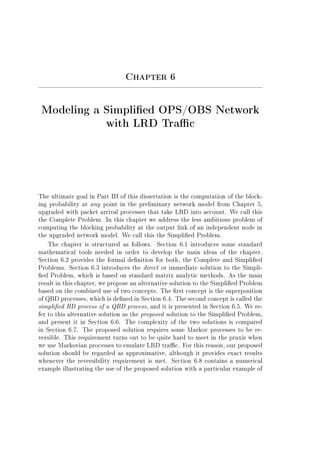
![106 Modeling a Simplied OPS/OBS Network with LRD Trac
packet arrival process emulating LRD. In this example the proposed solution is
approximative, and we empirically evaluate the accuracy of such approximation.
6.1 Mathematical Tools
This section completes the list of mathematical tools presented in Section 5.1 with
three additional denitions.
Denition 6.1.1 [105] A continuous phase-type random variable of order n rep-
resented as PH(τ, T) is dened as the time to absorption in an absorbing Markov
process with generator
0 0
t T
, (6.1)
and initial distribution (0 τ), where 0 and τ are row vectors of size n, and t is a
column vector of size n. The state 0 is the absorbing state.
In this chapter we use a Markov-Modulated Poisson Process (MMPP) in order
to emulate LRD trac. We dene a MMPP as follows [105]:
Denition 6.1.2 A MMPP with representation MMPP(D0, D1) is a MAP(D0, D1)
(see Section 5.1) where the matrix D1 is diagonal.
According to this denition, when a MMPP registers a packet arrival it in-
creases its level, but is not allowed to change its phase.
Quasi-birth-and-death (QBD) processes constitute a generalization of the BD
processes introduced in Section 5.1. In this generalization each level of the BD
is expanded into a series of states called phases. In particular, we present the
following denition [105].
Denition 6.1.3 A nonhomogeneous continuous-time QBD is a Markov process
{X(t), t ∈ R+
} on the two-dimensional state space {(n, p) : 0 ≤ n ≤ η ≤ ∞, 1 ≤
p ≤ ϕ(n) ∞} which we partition as ∪0≤n≤ηl(n), where l(n) = {(n, 1), (n, 2),
. . . , (n, ϕ(n))} for 0 ≤ n ≤ η. The innitesimal generator of the QBD is block-
tridiagonal and has the form:
Q =
Q
(0)
1 Q
(0)
0
Q
(1)
2 Q
(1)
1
...
... ... Q
(η−1)
0
Q
(η)
2 Q
(η)
1
. (6.2)](https://image.slidesharecdn.com/3f7f65b2-eeec-4afd-a395-b25a5ff55a20-160530113535/85/Modeling_Future_All_Optical_Networks_without_Buff-134-320.jpg)
![6.2 Problem Description 107
The rst coordinate n of a QBD is usually called the level, and the second
coordinate p is called the phase of the state (n, p). Notice from the denition that
the number η of levels might be nite or innite, and the number of phases ϕ(n)
is nite and may depend on the level n. In this denition X(t) represents the level
of the QBD as a function of t. In order to fully characterize X(t) not only level
but also phase transitions must be taken into account.
We assume throughout the remainder of this dissertation that all QBDs are
irreducible and positive recurrent. Then the system θQ = 0, θ1 = 1, has a unique
solution θ = (θ(0)
, θ(1)
, . . . , θ(η)
) referred to as the stationary distribution of the
QBD.
Given the n × m matrix A and the p × q matrix B, the Kronecker product
A ⊗ B is a np × mq matrix with the block structure [105]
A ⊗ B =
a1,1B · · · a1,mB
...
...
...
an,1B · · · an,mB
. (6.3)
We provide now some general guidelines to follow the notation used in this
chapter. The generators of all QBDs and their rate matrices are written with
the uppercase letter Q. The generators of all BDs and their rates are denoted
by lowercase q. The stationary distribution of QBD processes is written with the
symbol θ, whereas that of BD processes is written with δ.
6.2 Problem Description
As stated in the introduction, we refer by a Markovian pLRD process to the
superposition of a nite number of independent MMPPs. Numerous studies have
presented Markovian pLRD processes that emulate LRD trac [7, 176, 70, 120,
143]. These studies show that Markovian pLRD processes constitute simple and
yet accurate tools for mimicking LRD behavior. In our study, simplicity is needed
since we want to obtain tractable analytical results. Naturally, the accuracy of the
Markovian pLRD processes in [7, 176, 70, 120, 143] also constitutes an asset for
us. For this reason, in this chapter we have chosen the use of Markovian pLRD
processes as an approximation to the real LRD processes. Accordingly, we plan
to extend the preliminary stochastic network model introduced in Chapter 5 by
substituting each Poisson process with a Markovian pLRD packet arrival process.
In particular, we want to solve the following problem:
The Complete Problem: Compute the packet blocking probability
at any point in the stochastic network model from Chapter 5, up-](https://image.slidesharecdn.com/3f7f65b2-eeec-4afd-a395-b25a5ff55a20-160530113535/85/Modeling_Future_All_Optical_Networks_without_Buff-135-320.jpg)
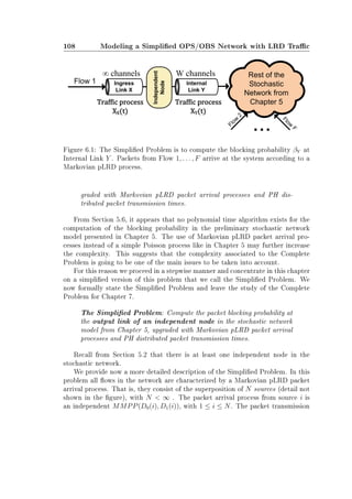
![6.2 Problem Description 109
times for packets arriving from each MMPP(D0(i), D1(i)), 1 ≤ i ≤ N are PH
distributed. The PH distribution is independent from any other arrival process
MMPP(D0(j), D1(j)), j = i and from its corresponding PH distributed packet
transmission times. However, it may be dierent for each source i.
Let us denote by link Y the output link of the independent node under study
(see Figure 6.1). This link is an internal link with W channels (see Section 5.2)
carrying packets that arrive at the independent node through M dierent input
links. Each input link is an ingress link with ∞ channels (see Section 5.2) receiving
packets directly from a single ow. For the ease of notation we assume hereinafter
that M = 1, and denote by link X the unique ingress link carrying packets from a
single ow, that we call Flow 1, to internal link Y (see Figure 6.1). This assumption
is not restrictive since the Simplied Problem with M ≥ 2 can be expressed as
an instance of the Simplied Problem with M = 1. Indeed, since each Markovian
pLRD is a superposition of nitely many MMPPs, the superposition of nitely
many Markovian pLRDs is automatically a superposition of nitely many MMPPs.
Blocking takes place in Figure 6.1 when a packet arriving at link Y nds all
its W channels busy with the transmission of other packets. The packet block-
ing probability βY at link Y as dened in Section 5.5.2 measures the stationary
probability that an arriving packet at this link is blocked.
Let us denote by {XX(t), t ∈ R+
} and {XY (t), t ∈ R+
} the trac process on
links X and Y , respectively. Observe that the sets TX and TY (see Section 5.4 for
a denition) on links X and Y , respectively have only one element corresponding
to Flow 1. That is, TX = TY = {1}. This implies that the trac process at links
X and Y can be obtained from Flow 1 exclusively, and that the computation of
the blocking probability at link Y can be isolated from the details of the rest of
the stochastic network in Chapter 5. This is implicitly shown in Figure 6.1 by
drawing the rest of the stochastic network as a network cloud, and constitutes a
considerable simplication with respect to the Complete Problem.
In spite of this simplication, we show in Section 6.7 that the computation of
βY in the Simplied Problem cannot be done in polynomial time with a state-of-
the-art approach that we call the direct solution. The reason for this is that the
state space of the trac process on link Y exponentially grows with the number
N of independent MMPPs being superposed.
As our main result in this chapter we overcome this intractability problem by
designing an algorithm for the computation of βY which exhibits a complexity
that linearly scales with N. We call this the proposed solution to the Simplied
Problem. The algorithm provides exact results under the assumption that the
trac processes on links X and Y are reversible (see Denition 5.1.2). In the
praxis, X and Y are not reversible with the Markovian pLRD processes presented
in [7, 176, 70, 120, 143]. For this reason we consider our algorithm to be approxi-](https://image.slidesharecdn.com/3f7f65b2-eeec-4afd-a395-b25a5ff55a20-160530113535/85/Modeling_Future_All_Optical_Networks_without_Buff-137-320.jpg)
![110 Modeling a Simplied OPS/OBS Network with LRD Trac
mative. In Section 6.8.3 we numerically show that our algorithm provides accurate
approximations with a particular Markovian pLRD obtained from [70].
6.3 The Direct Solution to the Simplied Problem
In this section we derive an expression for the computation of the blocking prob-
ability βY at link Y in Figure 6.1. Following Kendall's notation [101], link Y
can be regarded as a MMPP/PH/W/W queuing system. Since this system is
well-known, the results in this section are not new and we will not go into details.
Like in Chapter 5 we compute βY in three steps. First, we characterize the
trac process on links X and Y . Second, we compute the average arrival rate of
packets at links X and Y . Third, we provide an expression for the packet blocking
probability βY at link Y in Figure 6.1.
The trac process {XX(t), t ∈ R+
} on link X provides the number of simulta-
neous packet transmissions as a function of t (see Section 5.4). The packet arrival
process at link X is a MMPP that results from the superposition of N independent
MMPPs [61]. The packet transmission times at this link are PH distributed. Thus,
{XX(t), t ∈ R+
} corresponds to the level of a nonhomogeneous QBD process X
with ∞ levels and state space ∪n≥0l(n), where l(n) = {(n, 1), (n, 2), . . . , (n, ϕ(n))},
and ϕ(n) denotes the number of phases at level n. The trac process {XX(t), t ∈
R+
} is the superposition
XX(t) =
N
i=1
XX(i)(t), (6.4)
of N independent trac processes {XX(i)(t), t ∈ R+
}1≤i≤N . This result follows
immediately from the fact that packet arrivals and service times for source i are
independent from any other source j = i. The i-th trac process {XX(i)(t), t ∈
R+
} describes the number of busy channels as a function of time in an independent
ingress link with ∞ channels receiving packet arrivals from MMPP(D0(i), D1(i))
and their corresponding transmission times PH(τ(i), T(i)), for 1 ≤ i ≤ N. Thus,
{XX(i)(t), t ∈ R+
} is the QBD of the MMPP(D0(i), D1(i))/PH(τ(i), T(i))/∞/∞
system. We call this QBD X(i). Its innitesimal generator QX(i) is given by:
QX(i) =
Q
(0,X(i))
1 Q
(0,X(i))
0
Q
(1,X(i))
2 Q
(1,X(i))
1 Q
(1,X(i))
0
...
...
...
, (6.5)
with](https://image.slidesharecdn.com/3f7f65b2-eeec-4afd-a395-b25a5ff55a20-160530113535/85/Modeling_Future_All_Optical_Networks_without_Buff-138-320.jpg)
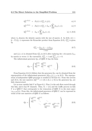
![112 Modeling a Simplied OPS/OBS Network with LRD Trac
where the o-diagonal elements in Q
(W,Y )
1 are equal to those in Q
(W,X)
1 and the
diagonal elements are set so that (Q
(W,X)
2 + Q
(W,Y )
1 )1 = 0. Another way for un-
derstanding the process of truncation is through the transition graph of QBD Y .
This transition graph is obtained from that of QBD X after eliminating all the
states corresponding to levels above W, together with the arcs that go from any
state in ∪0≤n≤W lY (n) to any state in ∪nW lY (n), and in the reverse direction.
Let us consider the average arrival rate rk of packets from Flow 1 at link k in
Figure 6.1, with k = {X, Y }, as dened in Denition 5.5.1. Notice that for the
ease of notation we have dropped the subindex 1 referring to Flow 1 with respect
to the notation in Chapter 5 (see Section 5.5).
The average arrival rate rX of packets from Flow 1 at link X can be expressed
as
rX =
N
i=1
rX(i), (6.10)
where rX(i) = ε(i)D1(i)1 represents the average arrival rate of MMPP(D0(i), D1(i))
from Flow 1 [105], and ε(i) is the stationary distribution associated to the MMPP
(see Section 5.1).
Proposition 6.3.1 The average arrival rate rY of packets from Flow 1 at link Y
is equal to
rY =
W−1
n=0
θ
(n)
Y Q
(n,X)
0 1, (6.11)
where θY = (θ
(0)
Y . . . θ
(W)
Y ) is the stationary distribution of QY .
Proof: The average arrival rate rY is equal to the average rate at which QBD Y
increases its level. When QBD Y is at level n and phase p it increases its level
with an average rate (Q
(n,Y )
0 1)p, where vp denotes the p-th element in vector v.
Thus, conditioning on the level and phase of QBD Y we conclude that the average
arrival rate rY is given by Equation (6.11).
The following proposition provides the direct solution to the Simplied Problem
in Section 6.2.
Proposition 6.3.2 The packet blocking probability βY at link Y is equal to:
βY = 1 −
rY
rX
, (6.12)
where rY and rX are the average arrival rates given by Equations (6.10) and (6.11).](https://image.slidesharecdn.com/3f7f65b2-eeec-4afd-a395-b25a5ff55a20-160530113535/85/Modeling_Future_All_Optical_Networks_without_Buff-140-320.jpg)
![6.4 The Superposition of 2 QBD Processes 113
Proof: We just provide the outline of the proof since it is analogous to that of
Proposition 5.5.4. The trac process at link Y is characterized in this case by
a QBD process, instead of by a multivariate BD process as in Proposition 5.5.4.
The proof proceeds in two steps. In the rst step it is proven that the trac
process at link Y observed at the arrival time of packets at this link is a stationary
Markov chain {Z[n], n ∈ N+
} (see Statement 5.5.3). As in Equation (5.18), the
packet blocking probability βY can be related to the stationary distribution γ =
(γ(0)
, . . . , γ(W)
) of {Z[n], n ∈ N+
} by means of
βY = 1 −
0≤n≤W−1
γ(n)
1.
In the second step the ergodic theorem for discrete-time Markov chains (see
[139, Proposition 2.12.4]) is used in order to relate the stationary distribution γ of
{Z[n], n ∈ N+
} to the quotient of rY over rX.
As stated in the previous section, the main goal of this chapter is to nd an al-
ternative method to compute the blocking probability βY . In particular, we focus
on the computation of rY since according to Section 6.7 it is the term in (6.12)
presenting the highest computational cost. In the following two sections we intro-
duce two mathematical tools on which the new method relies: the superposition
of QBDs and the simplied BD of a QBD process.
6.4 The Superposition of 2 QBD Processes
Let us consider two independent QBD processes A and B, and let {XA(t), t ∈ R+
}
and {XB(t), t ∈ R+
} denote, respectively, their visited level as a function of t. The
superposition of QBD processes A and B is another QBD process C such that its
level {XC(t), t ∈ R+
} will satisfy:
XC(t) = XA(t) + XB(t), (6.13)
for all t ∈ R+
. That is, QBD C increases/decreases its level whenever either QBD
A or QBD B increases/decreases its level, and QBD C is at level 0 i QBDs A and
B are both at level 0.
In this section we study in more detail the structure of QBD C as a function
of the parameters of QBDs A and B. Before addressing the general case, we begin
with a particular case in order to illustrate the concept of superposition. Let us
consider two independent BD processes a and b with innitesimal generators qa
and qb given by](https://image.slidesharecdn.com/3f7f65b2-eeec-4afd-a395-b25a5ff55a20-160530113535/85/Modeling_Future_All_Optical_Networks_without_Buff-141-320.jpg)
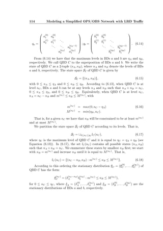
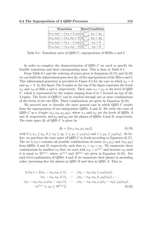
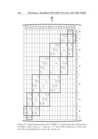
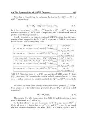
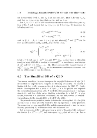
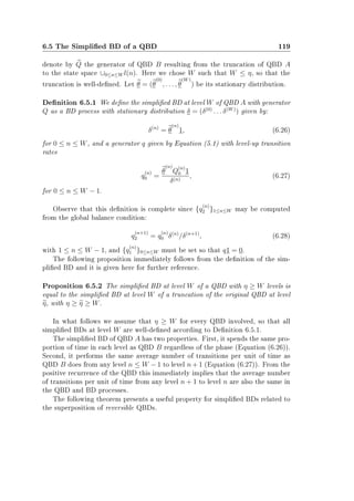
![120 Modeling a Simplied OPS/OBS Network with LRD Trac
Theorem 6.5.3 The simplied BD of the superposition of two independent re-
versible QBDs is equal to the simplied BD of the superposition of the simplied
BDs of each one of the two QBDs.
Proof: We denote by {Q
(n,X)
i , i ∈ {0, 1, 2}, 0 ≤ n ≤ ηX} the transition rate matrices
of a QBD X. The transition rates of a BD x are denoted by {q
(n,x)
i , i = {0, 1, 2}, 0 ≤
n ≤ W}. We also denote by θX = (θ
(0)
X , . . . , θ
(W)
X ) the stationary distribution of
the truncation of QBD X at level W.
We refer to Figure 6.3 for a diagram of the proof. According to this diagram,
we have two independent reversible QBDs A and B with generators QA and QB,
stationary distributions θA and θB, and ηA + 1 and ηB + 1 levels, respectively. We
denote by BD a and BD b their simplied BDs at level W, with generators qa and
qb and stationary distributions δa, δb, respectively. Let QBD C with stationary
distribution θC and ηC + 1 = ηA + ηB + 1 levels (see Equation (6.13)) be the
superposition of QBDs A and B. That is, QC = QA QB. Moreover, let QBD
D with stationary distribution θD be the superposition of BDs a and b. That is,
QD = qa qb. We want to prove that the generators qc and qd of the simplied
BDs c and d at level W of QBDs C and D, respectively, are equal (see Figure 6.3).
From Denition 6.5.1 it follows that both, BD c and d have W + 1 levels. We
proceed by proving that δc = δd and that {q
(n,c)
0 = q
(n,d)
0 , 0 ≤ n W}. From
Denition 6.5.1 we have that this univocally denes the rest of the parameters in
each generator qc and qd and implies their equality.
Let us begin with the proof that δc = δd. On the one hand we have δ
(n)
c = θ
(n)
C 1,
for 0 ≤ n ≤ W, which follows from Equation (6.26). Since QBDs A and B
are assumed to be reversible, so is QBD C and we have δ
(n)
c = ξ−1
C θ
(n)
C 1. with
ξC = W
n=0 θ
(n)
C 1 [144, Theorem 2.12].
Expanding the expression for θ
(n)
C according to Equation (6.21) leads to:
δ(n)
c = ξ−1
C
n
i=0
θ
(n−i)
A 1 · θ
(i)
B 1. (6.29)
On the other hand, we have for 0 ≤ n ≤ W that δ
(n)
d = θ
(n)
D 1, which follows from
Equation (6.26). QBD D is the superposition of two BD processes, and therefore
it is also reversible. Using this fact and [144, Theorem 2.12] gives δ
(n)
d = ξ−1
D θ
(n)
D 1,
with ξD = W
n=0 θ
(n)
D 1.
Expanding the expression for θ
(n)
D according to Equation (6.21) leads to:
δ
(n)
d = ξ−1
D
n
i=0
δ(n−i)
a δ
(i)
b . (6.30)](https://image.slidesharecdn.com/3f7f65b2-eeec-4afd-a395-b25a5ff55a20-160530113535/85/Modeling_Future_All_Optical_Networks_without_Buff-148-320.jpg)
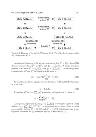
![122 Modeling a Simplied OPS/OBS Network with LRD Trac
We proceed now to prove that {q
(n,c)
0 = q
(n,d)
0 }0≤nW .
On the one hand, for 0 ≤ n W, q
(n,c)
0 can be expressed as:
q
(n,c)
0 =
θ
(n)
C Q
(n,C)
0 1
ξCδ
(n)
c
, (6.33)
which follows from Equation (6.27) and from the fact that QBD C is reversible.
The simplied BDs a and b at level W from QBDs A and B are well-dened
and so ηA ≥ W and ηB ≥ W (see Denition 6.5.1). Moreover, for 0 ≤ n ≤ W − 1
we have m(n)
= 0 and M(n)
= n (see Equation (6.16)). Thus, the conditions
n − m(n)
ηA and M(n)
ηB for Equation (6.25) in Section 6.4 are fullled. We
therefore expand Q
(n,C)
0 in Equation (6.33) from Equation (6.25). We also expand
θ
(n)
C according to Equation (6.21), which leads to:
q
(n,c)
0 =
n
i=0(θ
(n−i)
A ⊗ θ
(i)
B )[Q
(n−i,A)
0 ⊗ IQ
(i,B)
0
+ IQ
(n−i,A)
0
⊗ Q
(i,B)
0 ]1
ξCδ
(n)
c
,
where IA is the identity matrix of size equal to that of matrix A.
From the use of the distributive property of the Kronecker product over the
sum and of its matrix-multiplication property (A ⊗ B)(C ⊗ D) = (AC ⊗ BD), we
have:
q
(n,c)
0 =
n
i=0[θ
(n−i)
A Q
(n−i,A)
0 ⊗ θ
(i)
B + θ
(n−i)
A ⊗ θ
(i)
B Q
(i,B)
0 ]1
ξCδ
(n)
c
.
Identifying Equations (6.26) and (6.27) for the simplied BDs a and b and
using the fact that QBDs A and B are reversible processes leads to:
q
(n,c)
0 =
ξAξB
n
i=0 δ
(n−i)
a q
(n−i,a)
0 δ
(i)
b + δ
(n−i)
a δ
(i)
b q
(i,b)
0
ξCδ
(n)
c
. (6.34)
On the other hand, for 0 ≤ n W, q
(n,d)
0 can be expressed as:
q
(n,d)
0 =
θ
(n)
D Q
(n,D)
0 1
ξDδ
(n)
d
,
which derives from Equation (6.27) and the fact that QBD D is reversible.
Once again, the conditions n−m(n)
ηA and M(n)
ηB for Equation (6.25) in
Section 6.4 are fullled. We therefore substitute Q
(n,D)
0 by its equivalent expression
in Equation (6.33). We also expand θ
(n)
D according to Equation (6.21), which leads
to:](https://image.slidesharecdn.com/3f7f65b2-eeec-4afd-a395-b25a5ff55a20-160530113535/85/Modeling_Future_All_Optical_Networks_without_Buff-150-320.jpg)
![6.5 The Simplied BD of a QBD 123
q
(n,d)
0 =
n
i=0 δ
(n−i)
a δ
(i)
b [q
(n−i,a)
0 + q
(i,b)
0 ]1
ξDδ
(n)
d
=
n
i=0 δ
(n−i)
a q
(n−i,a)
0 δ
(i)
b + δ
(n−i)
a δ
(i)
b q
(i,b)
0
ξDδ
(n)
c
. (6.35)
The equality between Equations (6.34) and (6.35) follows immediately from
Equation (6.32).
We introduce now a new notation and represent by ΨW (Q) the generator of the
simplied BD at level W of a QBD with generator Q. Recall from Equation (6.22)
that the notation QA QB represents the superposition of QBDs A and B. With
this notation, we can rewrite Theorem 6.5.3 as:
ΨW (QA QB) = ΨW [ΨW (QA) ΨW (QB)], (6.36)
when QBDs A and B are the independent and reversible QBDs. This represen-
tation suggests that it is possible to extend Theorem 6.5.3 to any number N of
independent QBDs. This extension is built according to the following corollary.
Corollary 6.5.4 The simplied BD at level W with generator
q = ΨW (Q1 · · · QN ),
of the superposition of a number N of independent reversible QBDs with generators
{Qi}1≤i≤N fullls:
q = ΨW [ΨW (Q1 · · · QN−1) ΨW (QN )].
Proof: The proof follows immediately from Theorem 6.5.3 after identifying in
Equation (6.36) QA = Q1 · · · QN−1 and QB = QN .
We now propose an algorithm to compute the generator q of the BD obtained
by simplifying the superposition of a number N of QBD. Let us remark that
Equation (6.37) can be iteratively applied to ΨW (Q1 · · · QN−1), ΨW (Q1
· · · QN−2) and successive terms until we have the superposition ΨW (ΨW (Q1)
ΨW (Q2)). This leads to Algorithm 3.
The functioning of the algorithm is illustrated in Figure 6.4. Starting from the
innitesimal generators of the dierent QBDs the algorithm proceeds by iterating
two simple actions: First, compute simplied BD at level W of two QBDs. Second,
superpose the resulting pair of BD processes. When the for loop is over, the BD
with generator ΨW (Q1) is equal to q, by direct application of Corollary 6.5.4.](https://image.slidesharecdn.com/3f7f65b2-eeec-4afd-a395-b25a5ff55a20-160530113535/85/Modeling_Future_All_Optical_Networks_without_Buff-151-320.jpg)
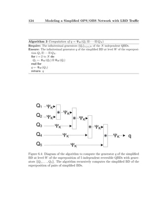
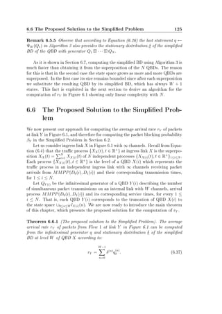
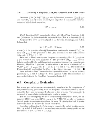
![6.7 Complexity Evaluation 127
In the computation of rX, common to both solutions, we exploit the fact that
the MMPP(D0, D1) is a superposition of N independent MMPPs and express rX
according to Equation (6.10). This equation requires the computation of ε(i), the
stationary distribution of the phase process associated to MMPP(D0(i), D1(i)),
which scales as O(ζ3
). Therefore, the complexity of the computation of rX is
O(N · ζ3
), showing only a linear increase of complexity with N.
The computation of rY is the most troublesome part, and it is where the
proposed solution provides improvement. According to the direct solution, rY is
computed from Equation (6.11). This requires to nd the stationary distribution
θY . That is, the unique non-negative solution to the system θY QY = 0, normalized
with θY 1 = 1. This system can be solved by means of the Linear Level Reduction
algorithm [105, 68], which is a version of the well-known Gaussian elimination
method that acknowledges the block-tridiagonal structure of QY . The complexity
of this method is O( 0≤n≤W K3
n), where Kn is the size of the matrix Q
(n,Y )
1 in the
generator QY . In our case it can be seen that Kn = ϑn
· ζN
since Q
(n,Y )
1 must keep
track of the phase associated to the service time of each one of the n packets in
the system and of the phase of each one of the N MMPPs. Notice that it is not
necessary to keep track in Q
(n,Y )
1 of the source that the packet occupying each one
of the busy servers comes from, since the service time distribution is by assumption
the same for all MMPP sources.
Let us dene S = 0≤n≤W ϑ3n
. That is, solving the sum we have:
S =
[1−ϑ3(W +1)]
[1−ϑ3]
if ϑ = 1
W + 1 otherwise
(6.40)
Then, the complexity of the direct solution for the computation of rY is
O(S · ζ3N
).
As it can be clearly appreciated, this complexity scales exponentially with
the number N of sources. This is very likely to lead to scalability problems for
moderate to large values of N if ζ 1. And usually, ζ 1 because if ζ = 1 we are
dealing with the trivial case in which each MMPP represents a Poisson process.
We now estimate the complexity of our solution in Theorem 6.6.1. It can
be observed from Figure 6.4 that Algorithm 3 performs the following operations,
listed with no specic order. Operation 1 consists of the computation of N − 1
superpositions of pairs of BD processes. Operation 2 consists of the computation
of N − 1 simplied BDs of QBDs that result from the superposition of a pair of
BD processes. Operation 3 consists of the computation of N simplied BDs, one
for each original QBD.
We begin with Operation 1. The superposition of a pair of BD processes is
computationally very ecient. This superposition results in a QBD process, and](https://image.slidesharecdn.com/3f7f65b2-eeec-4afd-a395-b25a5ff55a20-160530113535/85/Modeling_Future_All_Optical_Networks_without_Buff-155-320.jpg)
![128 Modeling a Simplied OPS/OBS Network with LRD Trac
its computation comprises two steps. The rst step leads to the characterization
of the level-up transition matrices of the QBD from levels 0 until W − 1 (see
Equation (6.25). Since the QBD is the superposition of two BDs, all Kronecker
products required in this step are with identity matrices (see Section 6.4). This
means that the coecients of the generators of the two BDs are just rearranged
according to the Kronecker operations, but that no scalar products take place (see
Figure 6.2). The second step leads to the characterization of the stationary distri-
bution of the QBD between levels 0 and W. The QBD has Kn = n + 1 phases at
level n, 0 ≤ n ≤ W (see Equation (6.18)). The value of the stationary distribution
at each phase is the result of a scalar product (see Equation (6.21)). Thus, the
number G of scalar products needed to compute the stationary distribution of the
superposition of two BDs is equal to 0≤n≤W n + 1. That is,
G =
1
2
W2
+
3
2
W + 1. (6.41)
Thus, the overall complexity of Operation 1 is O((N − 1) · G).
We address now the complexity of Operation 2; the computation of N −1 sim-
plied BDs at level W of the superposition of pairs of BD processes. The stationary
distribution of the QBD is known from Operation 1 (see Equation (6.21)). There-
fore, the computation of the simplied BDs with Equations (6.26) and (6.27) is
not expensive in terms of scalar products. More specically, Equation (6.26) does
not require the computation of any scalar product. Regarding Equation (6.27), it
requires the computation of Kn
2
scalar products, where Kn = n + 1 is the number
of phases at level n in every QBD, 0 ≤ n ≤ W − 1 (see Equation (6.18)). Thus,
the number J of scalar products needed to compute the level-up transition rates
in Equation (6.27) for each QBD in Operation 2 is equal to 0≤n≤W−1(n + 1)2
.
That is,
J = (
1
3
W2
+
1
2
W +
1
3
) · W. (6.42)
Thus, the overall complexity of Operation 2 is O((N − 1) · J).
Finally, we proceed with Operation 3, which requires the computation of a
number of N simplied BDs at level W. This requires the computation of the
stationary distribution of each one of the N QBDs with generators {QY (i)}1≤i≤N
(see Theorem 6.6.1). For each QBD Y (i), 1 ≤ i ≤ N we can use the linear level
reduction algorithm [105, 68], which scales with O( 0≤n≤W K3
n), where Kn is the
size of the matrix Q
(n,Y (i))
1 in the generator QY (i). Since QBD Y (i) is fed with a
single MMPP we have that Kn = ϑn
· ζ. Thus, the complexity of Operation 2 is
O(N · S · ζ3
), where S is dened in Equation (6.40).
Therefore, the overall complexity for computing rY with the proposed solution
in Theorem 6.6.1 is:](https://image.slidesharecdn.com/3f7f65b2-eeec-4afd-a395-b25a5ff55a20-160530113535/85/Modeling_Future_All_Optical_Networks_without_Buff-156-320.jpg)
![6.8 A Case Study with a Markovian pLRD Process 129
O((N − 1) · (G + J) + N · S · ζ3
), (6.43)
where G and J are given by Equations (6.41) and (6.42), respectively.
The conclusion is that Theorem 6.6.1 eectively reduces the exponential in-
crease of complexity with N of the direct solution to a linear increase.
Concerning the memory complexity of Algorithm 3, it is independent of N.
Indeed, the statement inside the for can be implemented with three matrices, A,
B and C in the following way. Assume for instance that Q1, obtained from the
previous iteration, is stored in matrix C. We then compute ϕW (C) and store
the result in matrix A. We read matrix Qi (e.g., from a le or from the input
parameter list) and store its result in matrix C. We compute ϕW (C) and store the
result in matrix B. We then compute ϕW (A B) and store the result in matrix
C. We are then ready to begin the next iteration.
6.8 A Case Study with a Markovian pLRD Process
We illustrate now the use of Theorem 6.6.1 with a particular Markovian pLRD
process taken from [70] in order to compute the blocking probability βY in the
Simplied Problem in Section 6.2. Recall from this section that a Markovian
pLRD process is dened as the superposition of N independent MMPPs, and it is
used in order to emulate LRD.
A Markovian ON/OFF process is a particular case of a MMPP. In [70] it
is proven that the superposition of an innite number of Markovian ON/OFF
processes may indeed be LRD. The authors provide also the transition matrices for
two examples of ON/OFF processes fullling this property. We take the transition
matrices of each source from Example 2 in [70]. According to this example an
ON/OFF source i, with i ∈ N is dened as a two-state discrete-time Markov chain
{Zi[n], n ∈ N} with irreducible and aperiodic transition matrix P(i):
P(i) =
1 − (1/(i + 1))p
(1/(i + 1))p
(1/(i + 1))q
1 − (1/(i + 1))q , (6.44)
where p, q ∈ R.
In the OFF state the process generates 0 packets/slot, and in the ON state it
generates 1 packet/slot. The duration of the ON state is geometrically distributed
with parameter βi = 1 − (1/(i + 1))q
. Similarly the duration of the OFF state is
geometrically distributed with parameter αi = 1 − (1/(i + 1))p
. The superposition
of an innite number of such ON/OFF sources is LRD i p 2q +1 and p ≥ q +1,
in which case, the Hurst parameter H is such that 1/2 H ≤ 1 and it is given by](https://image.slidesharecdn.com/3f7f65b2-eeec-4afd-a395-b25a5ff55a20-160530113535/85/Modeling_Future_All_Optical_Networks_without_Buff-157-320.jpg)
![130 Modeling a Simplied OPS/OBS Network with LRD Trac
H =
(3q − p + 1)
2q
. (6.45)
In what follows we dene and use a continuous-time version {Zi(t), t ∈ R+
} of
each discrete ON/OFF process {Zi[n], n ∈ N} in which the duration of a time slot
is substituted by an exponential distribution of parameter λ. Then, the duration
of the OFF period is equal to the sum of R exponential random variables with
parameter λ, where R is geometrically distributed with parameter 1 − αi. This
random sum of random variables is equal to an exponential random variable of
parameter λ(1 − αi). Using this fact, the process {Zi(t), t ∈ R+
} is a stationary
PH-renewal process with inter-renewal distribution PH(τ(i), T(i)), where:
T(i) =
−λ λ(1 − βi)
λ(1 − αi) −λ(1 − αi)
,
τ(i) = (1, 0).
(6.46)
Consider now a nite number N of such ON/OFF processes and denote {Z(t), t ∈
R+
} their superposition:
Z(t) =
N
i=1
Zi(t). (6.47)
This superposition constitutes an approximation of a LRD (i.e., second-order
self-similar) process.
LRD processes are typically characterized by three parameters: the Hurst pa-
rameter H, the average arrival rate m, and the coecient of variation a of the
number of arrivals falling in a constant interval of time [123]. The Hurst param-
eter of the LRD process approximated by {Z(t)} can be directly computed from
Equation (6.45). We proceed now to provide approximate expressions for the com-
putation of the other two parameters (i.e., m and a) of a LRD process from its
approximation {Z(t)}.
The average arrival rate m of the LRD process is approximated by means of the
average arrival rate m of {Z(t)}, which is simply equal to the sum of the arrival
rate of each source {Zi(t)}1≤i≤N :
m = λ
N
i=1
(i + 1)q
− 1
(i + 1)q + (i + 1)p
. (6.48)
In order to obtain from {Z(t)} a simple approximation a of the parameter a
of the LRD process we introduce a slight modication in the denition of a. This
modication consists in interpreting a as the coecient of variation of the number
of arrivals falling in an interval of time which is exponentially distributed with
parameter υ (in the original denition the interval was constant). The impact of](https://image.slidesharecdn.com/3f7f65b2-eeec-4afd-a395-b25a5ff55a20-160530113535/85/Modeling_Future_All_Optical_Networks_without_Buff-158-320.jpg)
![6.8 A Case Study with a Markovian pLRD Process 131
this modication is empirically evaluated in Section 6.8.3. We proceed now to
obtain an approximation a from {Z(t)} for this coecient of variation a.
We dene Mi as the number of packet arrivals from the stationary ON/OFF
source {Zi(t), t ∈ R+
} in an interval of length (t, t+W), where Υ has an exponen-
tial distribution with parameter υ, independent of the PH-renewal process. The
number of arrivals Mi has a geometric distribution with parameter
ζi = πi[υ(υI − T(i))−1
]1, (6.49)
where πi = (τ(i)T(i)−1
1)−1
τ(i)T(i)−1
is the stationary distribution of the PH-
renewal process (see Example 3.2.5 in [105]).
Consider now the superposition {Z(t)} of N ON/OFF sources. The coef-
cient of variation a of the number M = N
i=1 Mi of arrivals from {Z(t), t ∈
R+
} in an interval with exponential distribution of parameter υ is given by a =
V ar[M]/E[M], where V ar and E denote variance and mean, respectively. From
the independence of all ON/OFF sources, Mi is independent of Mj, for i = j, 1 ≤
i, j ≤ N. Thus, V ar[M] = N
i=1 V ar[Mi], which implies that
a =
N
i=1(1 − ζi)ζ−2
i
N
i=1 ζ−1
i
. (6.50)
6.8.1 Applying the Proposed Solution to the Simplied Prob-
lem
Let us consider the Simplied Problem in Section 6.2 as illustrated in Figure 6.1.
We assume that packets arrive at the ingress link X according to the superposi-
tion of N processes {Zi(t), t ∈ R+
}1≤i≤N and that packet transmission times are
exponentially distributed with parameter µ.
Notice that the i-th PH-renewal process dened in Equation (6.46) is also a
MMPP, for 1 ≤ i ≤ N. Indeed, the parameters of the i-th MMPP are D0(i) = T(i)
and D1(i) = t(i)τ(i), where t(i) = 0 − T(i)1. This process is a MMPP since from
Equation (6.46) we have that D1(i) is diagonal. Thus, the packet arrival process at
the system is a MMPP, superposition of N independent MMPPs (see Section 6.2).
From this and Proposition 6.5.2 we have that the number of busy servers in a
buerless system with W servers (W nite), arrival process {Zi(t), t ∈ R+
}, and
the above mentioned service times can be described by the truncated QBD Y (i)
from Equation 6.9. In particular, QBD Y (i) has an innitesimal generator QY (i)
with the following rate matrices:](https://image.slidesharecdn.com/3f7f65b2-eeec-4afd-a395-b25a5ff55a20-160530113535/85/Modeling_Future_All_Optical_Networks_without_Buff-159-320.jpg)
![132 Modeling a Simplied OPS/OBS Network with LRD Trac
Q
(j,Y )
1 (i) =
• λ(1 − βi)
λ(1 − αi) •
, 0 ≤ j ≤ W,
Q
(j,Y )
0 (i) =
λβi 0
0 0
, 0 ≤ j ≤ W − 1,
Q
(j,Y )
2 (i) =
jµ 0
0 jµ
, 1 ≤ j ≤ W,
(6.51)
where the symbol • represents a scalar, such that QY (i)1 = 0.
In this section we illustrate the use of Theorem 6.6.1 to compute the packet
blocking probability in a buerless system with W servers receiving packet arrivals
from the superposition of N independent MMPP sources dened in Equation (6.46)
with exponentially distributed service times. In particular, we use Algorithm 3 to
compute the simplied BD of QY (1) · · · QY (N), and then compute the packet
blocking probability with Equation (6.37).
Each QBD process Y (i) with generator QY (i) in Equation (6.51) is not re-
versible. For instance, the average number of direct jumps from an OFF state
at level j to an OFF state at level j + 1 is zero, since element (2, 2) in matrix
Q
(j,Y )
0 (i) is zero. However, the average number of direct jumps from an OFF state
at level j + 1 to an OFF state at level j can be dierent from zero, since element
(2, 2) in matrix Q
(j,Y )
2 (i) is dierent from zero. From this, the QBD processes
{Y (i)}1≤i≤N do not fulll the requirements for applying Theorem 6.6.1. Thus, for
the example in this section Theorem 6.6.1 constitutes an approximative method
for the computation of the packet blocking probability. One of the main objectives
of this section is to empirically evaluate the eciency of such an approximation in
Section 6.8.3.
6.8.2 The Fitting Process
We are given a trac trace consisting in a sequence of packet sizes and packet
arrival times. We want to t the parameters from the QBDs presented in the
previous section to the data from this trace.
The unknown parameters from all QBD processes {Y (i)}1≤i≤N are λ, µ, p and
q. The parameter µ can be directly tted to the average packet transmission time
E[transmission]. This is proportional to the average packet size E[size] from the
trace according to E[transmission] = E[size]/C, where C is the capacity of the
link through which trac is sent. The rest of the parameters (λ, p and q) are
tted with estimations H, m and a from the trace of the parameters H, m and a
characterizing a typical LRD process. We now describe each one in turn.
The estimation H of the Hurst parameter can be obtained from a variety of
estimators. We refer to [94] for a performance comparison of some of the most](https://image.slidesharecdn.com/3f7f65b2-eeec-4afd-a395-b25a5ff55a20-160530113535/85/Modeling_Future_All_Optical_Networks_without_Buff-160-320.jpg)
![6.8 A Case Study with a Markovian pLRD Process 133
important ones. The estimation m of the average arrival rate is obtained from
the inverse of the sample mean of the packet interarrival times in the trace. The
estimation a of the coecient of variation is taken from the sample mean and
variance of the number of arrivals from the trace falling in adjacent intervals of
which length constitute the samples from an exponential distribution of parameter
υ. As in the standard procedure with constant sized intervals, the model allows
for arbitrary choice of the size of the intervals. In our case we have chosen 1/υ to
be equal to the mean interarrival time in the trac trace.
Once we have the estimations H, m and a we t the parameters λ, p and q as
follows. The parameter p depends on q through H (Equation (6.45)), so only two
degrees of freedom q and λ remain available for tting m and a. Solving for λ in
Equation (6.48) and substituting its value in the generator given by Equation (6.51)
permits us to compute q from Equation (6.50). The value of λ is then obtained
form Equation (6.48).
6.8.3 A Numerical Example
We want to test the accuracy of the proposed solution in Theorem 6.6.1 with a
numerical example of practical interest. We proceed as follows. We t the QBD
processes {Y (i)}1≤i≤N presented in Section 6.8.1 to a well-known real IP trac
trace showing asymptotic second-order self-similar scaling behavior (i.e., LRD). In
particular, we work with the August 1989 Bellcore trace pAug of 106
interarrival
times, as measured by Leland et al. [107]. Although slightly dated, this data set
provides a well-known benchmark useful for examining the LRD of network trac.
For the tting process we use the Hurst parameter estimation H ≈ 0.8 from [140]
for this trace, and we estimate m and a according to the procedures described
in Section 6.8.2. Once the parameters of the QBD processes {Y (i)}1≤i≤N are
tted we compute the packet blocking probability βY in the Simplied Problem
in Section 6.2 using Theorem 6.6.1. This computation is an approximation of the
real value since the QBD processes {Y (i)}1≤i≤N dened in Section 6.8.1 are not
reversible.
In order to evaluate the eciency of this approximation we measure the packet
blocking probability in the Simplied Problem in Section 6.2 using simulation tech-
niques. In particular, we simulate a buerless system with W servers or channels,
which constitutes an equivalent model of internal link Y in Figure 6.1. According
to Section 6.8.1, packet transmission times are sampled from an exponential distri-
bution in the simulation. Packet arrival times are synthesized from an asymptotic
second-order self-similar (i.e., a LRD) trac model tted to the same BC trace.
This LRD trac model is the Beta Multifractal Wavelet Model (MWM Beta)
presented in [140] and used in Section 3.6. The reason for using the MWM Beta
model and not the original BC trace in the simulation is to be able to synthesize](https://image.slidesharecdn.com/3f7f65b2-eeec-4afd-a395-b25a5ff55a20-160530113535/85/Modeling_Future_All_Optical_Networks_without_Buff-161-320.jpg)
![134 Modeling a Simplied OPS/OBS Network with LRD Trac
Figure 6.5: Packet blocking probability as a function of the number of servers W
in the system for an utilization factor of ρ = 80 Erlangs. The MWM Beta/Exp
(Simulation) curve shows the 95%-condence intervals for 10 sample paths of 219
packet arrivals each.
packet arrival times for several simulations and to compute condence intervals for
the packet blocking probability. The particular choice of the MWM Beta model is
motivated by the following two facts. First, the MWM Beta produces a sequence of
positive values. This permits us to easily interpret these values as the interarrival
times of the arrival process. Other LRD models such as fractional Gaussian noise
(fGn) produce also negative values, and therefore are not so easy to interpret in
terms of interarrival times. Second, the accuracy of the MWM Beta model tted
to the same BC trace we are using has already been shown to be excellent in a
comparative study presented in [140].
In what follows we refer to the utilization factor ρ as the ratio of the aver-
age arrival rate rI of the input process to the service rate µ of the exponential
transmission times. The Erlang B formula is used as a representative value for the
extreme case in which LRD is ignored and the arrival process is Poisson.
Figures 6.5 and 6.6 show a performance comparison in terms of packet blocking
probability in the buerless system as a function of the number W of channels for](https://image.slidesharecdn.com/3f7f65b2-eeec-4afd-a395-b25a5ff55a20-160530113535/85/Modeling_Future_All_Optical_Networks_without_Buff-162-320.jpg)
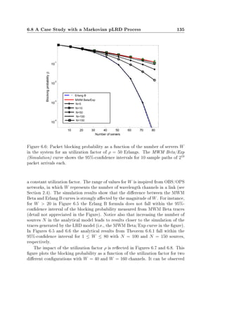
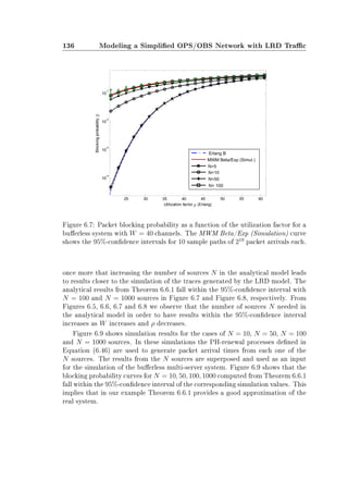
![6.8 A Case Study with a Markovian pLRD Process 137
Figure 6.8: Packet blocking probability as a function of the utilization factor for
a buerless system with W = 160 channels. The MWM Beta/Exp (Simulation)
curve shows the 95%-condence intervals for 100 sample paths of 222
packet arrivals
each.
We give now some insight into the reason why Theorem 6.6.1 provides in Fig-
ures 6.5, 6.6, 6.7 and 6.8 such a good approximation for large values of N to
the blocking probability in the buerless system with LRD input trac (i.e., the
MWM Beta/Exp curve in the gures). When the reversibility condition does not
hold, Theorem 6.5.3 is approximative since we cannot apply [144, Theorem 2.31]
in its proof. Theorem 2.31 in [144] states that the stationary distribution of a
reversible Markov process in a set A is proportional to the stationary distribution
of the truncation of this process to the set A. We refer hereinafter to this as the
property of proportionality. The property of proportionality is the only property
from reversible processes that is needed in order for Theorem 6.5.3, and ultimately
also Theorem 6.6.1, to be exact. We show now empirically that although the
QBD processes {Y (i)}1≤i≤N we are using are not reversible, they almost fulll the
property of proportionality. We argue that this is the reason why Theorem 6.6.1
provides such accurate results.
Let us proceed now with the description of the experimental setup. The main](https://image.slidesharecdn.com/3f7f65b2-eeec-4afd-a395-b25a5ff55a20-160530113535/85/Modeling_Future_All_Optical_Networks_without_Buff-165-320.jpg)
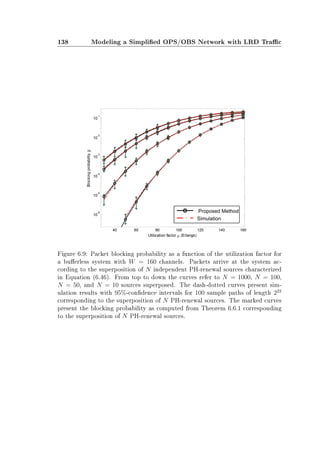
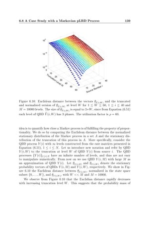
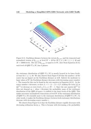
![6.8 A Case Study with a Markovian pLRD Process 141
mass of the stationary distribution of QBD Y (i, M) is shifted towards its lower
levels. This produces the same eect as in Figure 6.10. That is, it makes the
normalized truncation at level W of the stationary distribution of QBD Y (i, M)
resemble more to the stationary distribution of QBD Y (i, W), reducing their Eu-
clidean distance. The parameter i produces the same eect in Figure 6.11 as in
Figure 6.10. That is, the Euclidean distance between both stationary distributions
decrease with decreasing source number i.
The conclusion from Figures 6.10 and 6.11 is that as W increases and ρ de-
creases, the Euclidean distance decreases and thus Theorem 6.6.1 provides a better
approximation to the packet blocking probability in our experimental setup. In
the praxis, the parameter W is the number of servers or channels in the buerless
system under study. Therefore, Figure 6.10 suggests that the larger the number
of servers in the buferless system the more accurate is the approximative analysis
for LRD trac presented in Section 6.8. This result is extremely convenient since
in most cases of interest the number W of servers in the system under study is
rather large. For instance, in OBS/OPS networks W represents the number of
wavelengths in the DWDM ber and it may be equal to 40, 80 or even 160 [26, 67].
Regarding the value of ρ, it is limited by the maximum blocking probability
admissible in the OBS network. Let us take the example in Figure 6.7 with W = 40
wavelength channels. The value ρ = 30 Erlangs leads to a blocking probability of
around 10−1
, which is considered to be high for OBS networks. Even such high
value of ρ leads to an Euclidean distance in Figure 6.11 below 10−5
in the worst case
(i.e., for source number 40). This eect, and the relatively high value of W may
account for the high accuracy of Theorem 6.6.1 observed in Figures 6.5, 6.6, 6.7
and 6.8.](https://image.slidesharecdn.com/3f7f65b2-eeec-4afd-a395-b25a5ff55a20-160530113535/85/Modeling_Future_All_Optical_Networks_without_Buff-169-320.jpg)

![Chapter 7
Modeling a Buerless OPS/OBS Network
with LRD Trac
In this chapter we address the Complete Problem in Section 6.2. That is, we
study the preliminary network model presented in Chapter 5, upgraded with a
Markovian pLRD (pseudo LRD) packet arrival process and PH distributed packet
transmission times, as introduced in Chapter 6. The aim is to compute the blocking
probability at any point in the network.
The chapter is structured as follows. Section 7.1 provides a possible solution
to the Complete Problem, based on standard matrix analytic methods from [105]
and techniques from the theory of stochastic networks from [144]. This solution is
denoted as the direct solution to the Complete Problem. Section 7.2 presents an
alternative solution to the Complete Problem, based on the results on the simplied
BD of a QBD process presented in Chapter 6. This solution is denoted as the
proposed solution to the Complete Problem. Section 7.3 presents a comparative
study of the complexity associated to both, the direct and proposed solutions to
the Complete Problem. In Section 7.4 we make some numerical experiments in
order to study the accuracy of the proposed solution in an example where this
solution is approximative.
7.1 The Direct Solution to the Complete Problem
In this section we provide a possible solution to the Complete Problem in Sec-
tion 6.2, which we refer hereinafter to as the direct solution. The main assumption
is that the Markovian pLRD packet arrival processes and PH distributed packet](https://image.slidesharecdn.com/3f7f65b2-eeec-4afd-a395-b25a5ff55a20-160530113535/85/Modeling_Future_All_Optical_Networks_without_Buff-171-320.jpg)
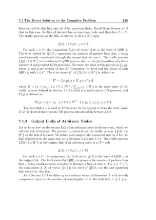
![146 Modeling a Buerless OPS/OBS Network with LRD Trac
Then, the trac process {X(t)} is a multivariate QBD process subject to the
constraint of a restricted state space E (w), given by:
E (w) = {(x, p), x ∈ E(w), p ∈ P(x)},
where
E(w) = {x = (xj : j ∈ T) ∈ N|T|
: Ax ≤ w}, (7.1)
is equal to the state space of the trac process dened in Section 5.4.3 (which is
a multivariate BD process), and P(x) is dened as
P(x) = {p = (pj : j ∈ T) ∈ N|C|
: 1 ≤ pj ≤ ϕj(xj), j ∈ T}. (7.2)
As in Section 5.4.3, the nontrivial equations in the system Ax ≤ w represent
constraints associated to the link of interest and to each one of its upstream links.
Each constraint imposes that the sum of the number of packets from the ows in
T routed through a given link must be below or equal than the number of channels
W in the link.
Since the trac process {X(t)} is the juxtaposition of a number of reversible
processes (see Section 7.1.2) subject to the constraint of a restricted state space
E (w) we conclude from Propositions 2.12 and 2.14 in [144] (see also Section 5.1)
that {X(t)} is a reversible process with product-form stationary distribution
Θ(x, p) =
1
h (w) m∈T
θm(xm, pm), (7.3)
for (x, p) ∈ E (w), where θm(xm, pm) is the stationary distribution of QBD m
measured at state (xm, pm), and h (w) is a normalization constant, equal to
h (w) =
x∈E(w) m∈T
θ(xm)
m 1. (7.4)
7.1.4 The Blocking Probability
In this section we provide several expressions for the computation of the packet
blocking probability measured at dierent points in the stochastic network under
study. This constitutes the direct solution to the Complete Problem on page 107.
The structure and results of this section for QBD processes are entirely analogue
to those of Section 5.5 for BD processes. For this reason we just present the outline
of the proofs, highlighting the dierences to the corresponding proofs in Section 5.5.
As in Section 5.5 we add a subindex k, 1 ≤ k ≤ L to the notation introduced
in the previous sections in order to be able to distinguish among dierent links in](https://image.slidesharecdn.com/3f7f65b2-eeec-4afd-a395-b25a5ff55a20-160530113535/85/Modeling_Future_All_Optical_Networks_without_Buff-174-320.jpg)
![7.1 The Direct Solution to the Complete Problem 147
the network. We begin with the computation of the average arrival rate rj,k
of packets from ow j at link k. The superindex is used once more in order
to dierentiate from the corresponding result for multivariate BD processes in
Chapter 5 (in this case Proposition 5.5.2).
Let Nj,k(t) denote the number of packets from ow j arriving at link k during
(0, t], 1 ≤ j ≤ F, 1 ≤ k ≤ L, t ∈ R+
. According to Denition 5.5.1 re refer to
rj,k as the time average rj,k(t) = t−1
Nj,k(t), when t → ∞. As in the previous
sections, the level of QBD j denotes the trac process at an ingress link of type
j, 1 ≤ j ≤ F.
Proposition 7.1.1 The average arrival rate of packets from ow j, j ∈ Ck at link
k converges w.p. 1 to the constant
rj,k =
(x,p)∈Ek(w−Akej)
Θk(x, p)
ϕj(xj+1)
z=1
(Q
(xj,j)
0 )pj,z, (7.5)
where ej denotes a vector of zeros with value one at position j, ϕj(x) denotes the
number of phases at level x of QBD j and (Q
(x,j)
0 )a,b denotes the element on the
a-th row and b-th column of the rate matrix Q
(x,j)
0 of the generator Qj of QBD j.
Proof: One way of proving this result is by adapting the proof of Proposition 5.5.2
to the case in which the trac process is a multivariate QBD process instead of
a multivariate BD process. This adaptation is rather straightforward, the main
dierence being that the state space of the trac process is made of two vectors
(x, p) instead of just one x.
We provide here the outline of an alternative proof based on probabilistic ar-
guments. The average arrival rate rj,k for packets from source j at link k is equal
to the average number of allowed transitions of the trac process on link k of the
form (x, p) → (x + ej, p†
), where the vector p†
is equal to the vector p except for a
possible change of phase at its j − th component, j ∈ Ck. Here the term allowed
means that the transition takes place between two states that belong to Ek(w).
This is ensured by making the initial state (x, p) belong to Ek(w − Akej). The av-
erage number of such transitions per unit of time is equal to the proportion of time
Θk(x, p) that the trac process spends at each state (x, p) ∈ Ek(w − Akej) times
the conditional rate at which the trac process registers the arrival of a packet
from source j when it is on state (x, p). This conditional rate is equal to the rate
at with which the j-th component Xj,k(t) of the trac process {Xk(t), t ∈ R+
}
makes a transition from level xj and phase pj to level xj + 1 whatever the change
of phase, that is,
ϕj(xj+1)
z=1 (Q
(xj,j)
0 )pj,z.
We are now ready to provide the direct solution to the Complete Problem on
page 107.](https://image.slidesharecdn.com/3f7f65b2-eeec-4afd-a395-b25a5ff55a20-160530113535/85/Modeling_Future_All_Optical_Networks_without_Buff-175-320.jpg)
![148 Modeling a Buerless OPS/OBS Network with LRD Trac
Proposition 7.1.2 The following list provides expressions for the packet blocking
probability at three dierent points in the network.
i. The packet blocking probability βj,O for ow j at the output link O of an
arbitrary node is given by
βj,O = 1 −
rj,O
rj,I
,
where rj,O and rj,I are the average arrival rates given by Equation (7.5)
of packets from ow j at the output O and input I links, respectively (see
Figure 5.2).
ii. The packet blocking probability βO at the output link O of an arbitrary node
is given by
βO = 1 −
j∈CO
rj,O
k∈I j∈Ck∩CO
rj,k
,
where I is the set of input links to the node carrying at least one ow in CO,
and rj,O and rj,k are given by Equation (7.5).
iii. The packet blocking probability βj for ow j is given by
βj = 1 −
rj,O
λj
,
where rj,O is given by Equation (7.5), O is the last link in the path of ow j,
and λj is the average arrival rate for packets from ow j.
Proof: We provide only an outline of the proof for the rst statement in the
proposition, since it is analogous to that of Proposition 5.5.4. The proof for the
other two statements is omitted since it is analogous to that of Propositions 5.5.5
and 5.5.6.
The proof of the rst statement proceeds in two steps. In the rst step it is
proven that the trac process at link O observed at the arrival time of packets
from ow j at this link is a stationary Markov chain {Zj,O[n], n ∈ N+
} (see State-
ment 5.5.3). As in Equation (5.18), the packet blocking probability βj,O can be re-
lated to the stationary distribution γj,O
= (γj,O(x, p))(x,p)EO(w) of {Zj,O[n], n ∈ N+
}
by means of
βj,O = 1 −
(x,p)∈EO(w−AOej)
γj,O(x, p).
In the second step the ergodic theorem for discrete-time Markov chains (see
[139, Proposition 2.12.4]) is used in order to relate the stationary distribution γj,O
of {Zj,O[n], n ∈ N+
} to the quotient of rj,O over rj,I.](https://image.slidesharecdn.com/3f7f65b2-eeec-4afd-a395-b25a5ff55a20-160530113535/85/Modeling_Future_All_Optical_Networks_without_Buff-176-320.jpg)
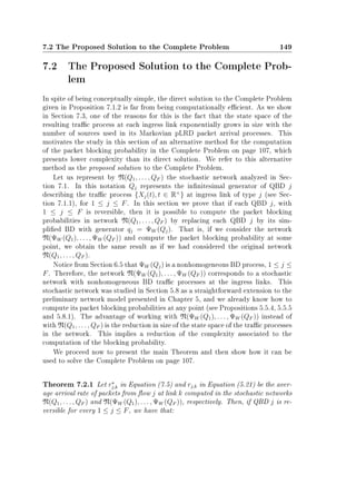
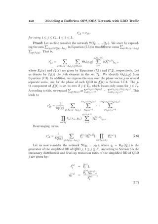
![7.2 The Proposed Solution to the Complete Problem 151
where θ
(x)
j represents the stationary distribution at level x of the truncation at level
W of QBD j, as dened in Section 6.9. Using the fact that QBD j is reversible,
we make use of [144, Theorem 2.31] and express the parameters of the simplied
BD j as a function of QBD j, instead of its truncated version at level W:
δ
(x)
j = ξ−1
j θ
(x)
j 1, (7.8)
q
(x,j)
0 = ξ−1
j
θ
(x)
j Q
(x,j)
0 1
δ
(x)
j
, (7.9)
where ξj = W
n=0 θ
(n)
j 1, 0 ≤ x ≤ W.
Identifying Equations (7.8) and (7.9) in the expression for rj,k in Equation (5.21)
leads to
rj,k =
m∈Tk
ξ−1
m
hk(w)
x∈Ek(w−Akej)
θ
(xj)
j Q
(xj,j)
0 1
m∈Tk,m=j
θ(xm)
m 1, (7.10)
where hk(w) is dened in Equation (5.9).
Comparing Equations (7.10) and (7.6) we conclude that rj,k = rj,k i
hk(w) =
m∈Tk
ξmhk(w). (7.11)
We now proceed to prove this equality. Starting from the denition of hk(w)
in Equation (7.4) we expand the sum as
hk(w) =
x∈Ek(w) p∈Pk(x) m∈Tk
θm(xm, pm).
Expanding the sum p∈Pk(x) according to each one of the components pj of p
with j ∈ Tk, and rearranging terms
hk(w) =
x∈Ek(w) m∈Tk
ϕm(xm)
pm=1
θm(xm, pm). (7.12)
According to Equation (7.8), the inner sum in Equation (7.12) is equal to
ξmδ
(xm)
m . Taking this into account and rearranging terms leads to
hk(w) =
m∈Tk
ξm
x∈Ek(w) m∈Tk
δ(xm)
m .](https://image.slidesharecdn.com/3f7f65b2-eeec-4afd-a395-b25a5ff55a20-160530113535/85/Modeling_Future_All_Optical_Networks_without_Buff-179-320.jpg)
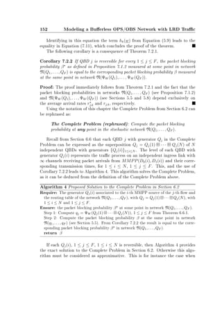
![7.3 Complexity Evaluation 153
we are using the Markovian pLRD process from Section 6.8. Observe that if the
reversibility condition does not hold, the direct solution to the Complete Problem
in Section 7.1 is also approximative.
In the following section we analyze the complexity associated to the direct and
proposed solutions to the Complete Problem.
7.3 Complexity Evaluation
Recall that W is the number of channels per link, N is the number of sources
per ow, F is the number of ows and L is the number of links in the network.
For convenience we make the same two assumptions as in Section 6.7. First,
the parameters {D0(i)}1≤i≤N and {D1(i)}1≤i≤N of the N MMPPS are all ζ × ζ
matrices. Second, packet transmission times have all the same PH distribution
with ϑ phases, independently of the MMPP the packet comes from.
We begin with the direct solution presented in Section 7.1. This solution re-
quires knowledge of the stationary distribution θj of each QBD j, 1 ≤ j ≤ F.
According to Section 6.7 each θj can be computed with Gaussian elimination in
O(S · ζ3N
) time, where S is given by Equation (6.40). Thus, the computation of
{θj}1≤j≤F scales with O(F · S · ζ3N
).
Once {θj}1≤j≤F are known the direct solution requires the computation of the
blocking probability at some point in network N(Q1, . . . , QF ). According to [129,
29], this presents a complexity of O(F · ( 0≤nW Kn)L
), where Kn = ϑn
· ζN
,
dened in Section 6.7, is the number of states in each QBD j at level n. According
to this, 0≤nW Kn = ζN
· H, where H = 0≤nW ϑn
, that is:
H =
[1−ϑW ]
[1−ϑ]
if ϑ = 1
W otherwise
(7.13)
The overall complexity of the direct solution is therefore of
O(F · [S · ζ3N
+ (ζN
· H)L
].) (7.14)
According to Equation (6.43) the rst step in the proposed solution in Algo-
rithm 4 has a complexity O(F · [(N − 1) · (G + J) + N · S · ζ3
]), where G and J are
given by Equations (6.41) and (6.42), respectively. The second step requires the
computation of the blocking probability at some point in the stochastic network
N(q1, . . . , qF ) from Chapter 5. According to Section 5.6 this step has a complexity
of O(F · WL
).
The overall complexity of the proposed solution is therefore of
O(F · [(N − 1) · (G + J) + N · S · ζ3
+ WL
].) (7.15)](https://image.slidesharecdn.com/3f7f65b2-eeec-4afd-a395-b25a5ff55a20-160530113535/85/Modeling_Future_All_Optical_Networks_without_Buff-181-320.jpg)
![154 Modeling a Buerless OPS/OBS Network with LRD Trac
Comparing the complexity of both solutions we observe that in the direct so-
lution the dependency with N is exponential, while in the proposed solution it is
linear. This permits to solve the Complete Problem on page 107 with basically the
same complexity as the computation of the blocking probability in the preliminary
stochastic network from Chapter 5, i.e., without Markovian pLRD arrival processes
and PH-distributed transmission times. More specically, the complexity of the
proposed solution is equal to that of the computation of the blocking probabil-
ity in the preliminary stochastic network from Chapter 5 plus an additional term
O(F · [(N − 1) · (G + J) + N · S · ζ3
]).
7.4 Numerical Study
In this section the stochastic network presented in this chapter is used in order
to model the network topology from Figure 5.3 in Chapter 5 with the routing
table from Table 5.2. We use the pLRD trac process introduced in Section 6.8
in order to model the arrival of packets from the dierent ows in the network.
Packet transmission times are exponentially distributed and thus the trac process
on an ingress link is given by the QBD process from Equation (6.51). According to
Section 6.8.1, this QBD is not reversible. This means that when the pLRD trac
process from Section 6.8 is used, the direct and proposed solutions presented in
Sections 7.1 and 7.2 of this chapter are approximative. Our main objective in this
section is to show with numerical examples the eciency of our proposed solution
as an approximation to the real blocking probability. In addition, we want to
compare the results with those from the network model presented in Chapter 5,
where trac is described by a Poisson process instead of by an pLRD process.
The purpose of this comparison is to quantify the impact of having pLRD instead
of Poisson trac in the network.
In this section we compute the blocking probability at dierent points in the
network scenario from Figure 5.3 using four dierent methods. The rst method
corresponds to the simulation of the network in Figure 5.3. In this simulation
packet transmission times are sampled from an exponential distribution. As in
Section 6.8.3, packet arrival times are synthesized from the MWM Beta LRD
process presented in Section 3.6. This process is tted to the well-known Bellcore
trace from Section 3.5.2. The blocking probability values obtained by this method
are presented in Figures 7.1, 7.2 and 7.3 under the Simulation LRD Trac label.
The second method corresponds to the proposed solution presented in Sec-
tion 7.2 of this chapter. We use the pLRD process from Section 6.8 and describe
the trac arriving from each ow in the network as the superposition of N = 1000
independent ON/OFF Markovian sources. According to Step 1 of Algorithm 4, we
compute for each ow the simplied BD at level W of the QBD representing the](https://image.slidesharecdn.com/3f7f65b2-eeec-4afd-a395-b25a5ff55a20-160530113535/85/Modeling_Future_All_Optical_Networks_without_Buff-182-320.jpg)
![7.4 Numerical Study 155
Figure 7.1: Blocking probability β3 for ow 3 as a function of the average load for
this ow for W = 8 channels.
trac process of this ow at its ingress link. The trac processes in the resulting
stochastic network can be described in terms of multivariated BD processes, as in
Chapter 5. Thus, we apply the same Monte Carlo simulation techniques from [103]
in order to estimate the blocking probability values. These values are presented
in Figures 7.1, 7.2 and 7.3 under the MC pLRD Trac label. As in Section 5.7,
500 simulations are used, each one with n = 15000 samples for the estimation of
the value of each partition function. Due to the high number of simulations the
95%-condence intervals are too small to be seen in Figures 7.1, 7.2 and 7.3. For
this reason they have been removed.
Notice that the two methods presented above acknowledge the LRD nature
of trac in our network, which is in accordance with our results from Part II of
this dissertation. The third and fourth methods completely ignore these results
and model incoming trac from each ow in the network with an independent
Poisson process. In particular, the third method uses the Monte Carlo simula-
tion techniques from [103] in order to estimate the blocking probability values in
the stochastic network model from Chapter 5. These values are presented in Fig-
ures 7.1, 7.2 and 7.3 under the MC Poisson Trac label. The fourth method uses
the Erlang xed-point approximation in order to approximate the values of the](https://image.slidesharecdn.com/3f7f65b2-eeec-4afd-a395-b25a5ff55a20-160530113535/85/Modeling_Future_All_Optical_Networks_without_Buff-183-320.jpg)
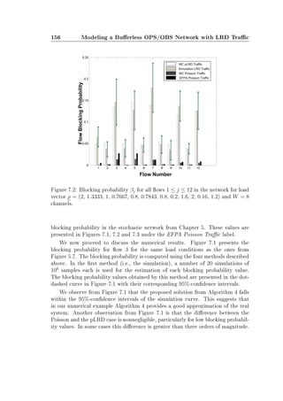
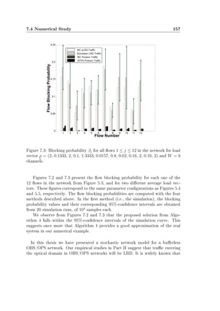
![158 Modeling a Buerless OPS/OBS Network with LRD Trac
LRD has a signicant negative impact on network performance, measured in terms
of such parameters as the buer dynamics and blocking probability [126, 63]. Our
results in Figures 7.1, 7.2 and 7.3 agree with this conclusion, reporting an increase
in the blocking probability which can be of several orders of magnitude.
According to these results, a very important characteristic of the stochastic
network model presented in this chapter is the fact that it can take LRD trac
into account. More specically, in this model we can emulate LRD trac by means
of the superposition of N independent MMPPs. Our empirical studies in Chapter
6 indicate that the accuracy of our approximation to LRD trac increases with
N. The fact that the complexity of this approximation increases only linearly with
N allows us to work with high values of N in order to reduce the approximation
errors.
The numerical experiments from this section take advantage from this fact and
use the superposition of N = 1000 independent ON/OFF sources in order to de-
scribe trac arriving from each ow in the network. The comparison of the results
obtained from Algorithm 4 and the simulation results in Figures 7.1, 7.2 and 7.3
permits us to conclude that in our numerical experiment the use of the Monte
Carlo techniques from [103] provides an estimation of the blocking probability
within the 95%-condence intervals.](https://image.slidesharecdn.com/3f7f65b2-eeec-4afd-a395-b25a5ff55a20-160530113535/85/Modeling_Future_All_Optical_Networks_without_Buff-186-320.jpg)


![Bibliography
[1] P. Abry, P. Flandrin, M.S. Taqqu, and D. Veitch. Self-Similar Network
Trac and Performance Evaluation, chapter Wavelets for the analysis, esti-
mation, and synthesis of scaling data, pages 3988. Wiley, 2000.
[2] P. Abry, P. Flandrin, M.S. Taqqu, and D. Veitch. Theory and Applications of
Long-Range Dependence, chapter Self-similarity and long-range dependence
through the wavelet lens, pages 527556. Birkhäuser, 2002.
[3] P. Abry, D. Veitch, and P. Flandrin. Long-range dependence: Revisiting
aggregation with wavelets. Journal of Time Series Analysis, 19:253266,
May 1998.
[4] G. P. Agrawal. Fiber-Optic Communications Systems. John Wiley and Sons,
2002.
[5] N. Akar and E. Karasan. Exact calculation of blocking probabilities for
buerless optical burst switched links. In BROADNETS, pages 110117,
San Jose, USA, October 2004.
[6] G. Alibert, F. Delorme, P. Boulet, J. Landreau, and H. Nakajima. Sub-
nanosecond tunable laser using a single electroabsorption tuning super struc-
ture grating. IEEE Photonics Technology Letters, 9:895897, July 1997.
[7] A. T. Andersen and B. F. Nielsen. A markovian approach for modeling
packet trac with long-range dependence. IEEE Journal on Selected Areas
in Communications, 16:719732, 1998.](https://image.slidesharecdn.com/3f7f65b2-eeec-4afd-a395-b25a5ff55a20-160530113535/85/Modeling_Future_All_Optical_Networks_without_Buff-189-320.jpg)
![162 Bibliography
[8] J. Aracil, M. Izal, D. Morato, and E. Magana. Multiresolution analysis of op-
tical burst switching trac. In IEEE International Conference on Networks
(ICON), pages 409 412, Sydney, 2003.
[9] R. Balakrishnan and C. Williamson. A performance comparison of monofrac-
tal and multifractal trac streams. In Proceedings of MASCOTS, pages
214226, 2000.
[10] K. Bergman. Overview of high capacity optical cross-connects. In Proceedings
of the 14th Annual Meeting of the IEEE LEOS, volume 1, pages 224225,
November 2001.
[11] A. Bergonzo, J. Jacquet, D. De Gaudemaris, J. Landreau, A. Plais, A. Vuong,
H. Sillard, T. Fillion, O. Durand, H. Krol, A. Accard, and I. Riant. Widely
vernier tunable external cavity laser including a sampled ber bragg grat-
ing with digital wavelength selection. IEEE Photonics Technology Letters,
15:11441146, August 2003.
[12] G. Bernstein, B. Rajagopalan, and D. Saha. Optical Network Control: Ar-
chitecture, Protocols, and Standards. Addison Wesley, 2004.
[13] A. Bhardwaj, J. Gripp, Simsarian J.E., and M. Zirngibl. Long-term wave-
length switching measurements with random schedules on fast tunable lasers.
In Proceedings of European Conference on Optical Communication (ECOC),
2002.
[14] A. Bragg, I. Baldine, and D. Stevenson. A transport layer architectural
framework for optical burst switched networks. In Proceedings of WOBS,
Dallas, TX, USA, October 2003.
[15] P. Bremaud. Markov Chains, Gibbs Fields, Monte Carlo Simulation and
Queues. Springer Verlag, 1991.
[16] H. Buchta. Analysis of Physical Constraints in an Optical Burst Switch-
ing Network. PhD thesis, Elektrotechnik und Informatik der Technischen
Universität Berlin, April 2005.
[17] D. Y. Burman, J. P. Lehoczky, and Y. Lim. Insensitivity of blocking proba-
bilities in a circuit-switching network. Journal of Applied Probability, 21:850
859, December 1984.
[18] C. S. Burrus, R. A. Gopinath, and H. Guo. Introduction to Wavelets and
Wavelet Transforms: A Primer. Prentice Hall, New Jersey, 1998.](https://image.slidesharecdn.com/3f7f65b2-eeec-4afd-a395-b25a5ff55a20-160530113535/85/Modeling_Future_All_Optical_Networks_without_Buff-190-320.jpg)
![Bibliography 163
[19] Y. Calabretta, N. AndLiu, M.T. Hill, H. de Waardt, G.D. Khoe, and H.J.S.
Dorren. All-optical header processor for packet switched networks. In IEE
Optoelectronics, pages 219223, 2003.
[20] A. Calogero. On the discrete wavelet transform of stochastic processes. Tech-
nical Report 1, Università e Politecnico di Torino, 2003.
[21] A. Calvo Devesa. Analysis of broadband trac traces. Master's thesis,
Faculté des Sciences Appliquées, ULB, 2007.
[22] J. Cao, W. S. Cleveland, D. Lin, and D. X. Sun. Internet trac tends toward
poisson and independent as the load increases. Nonlinear Estimation and
Classication, 6, 2002.
[23] J. Cao and K. Ramanan. A poisson limit for buer overow probabilities.
In IEEE INFOCOM, volume 2, pages 994 1003, 2002.
[24] X. Cao, J. Li, Y. Chen, and C. Qiao. TCP/IP packets assembly over optical
burst switching network. In Proceedings of GLOBECOM, volume 3, pages
28082812, 2002.
[25] M.C. Cardakli, D. Gurkan, S.A. Havstad, A.E. Willner, K.R. Parameswaran,
M.M. Fejer, and I. Brenner. All-optical time-slot-interchange and wavelength
conversion using dierence-frequency-generation and FBGs. In Proceedings
of Optical Fiber Communication Conference (OFC), volume 4, pages 196
198, March 2000.
[26] Y. Chen, C. Qiao, and X. Yu. Optical burst switching: a new area in optical
networking research. IEEE Network, 18:1623, May 2004.
[27] Y. Chen, H. Wu, D. Xu, and C. Qiao. Performance analysis of optical
burst switched node with deection routing. In Proceedings of IEEE ICC,
volume 2, pages 13551359, 2003.
[28] J. Cheyns, C. Develder, E. Van Breusegem, D. Colle, F. De Turck, P. Lagasse,
M. Pickavet, and P. Demeester. Clos lives on in optical packet switching.
IEEE Communications Magazine, 42:114 121, 2004.
[29] G. L. Choudhury, K. K. Leung, and W. Whitt. An inversion algorithm to
compute blocking probabilities in loss networks with state-dependent rates.
IEEE/ACM Transactions on Networking, 3:585601, October 1995.
[30] J. Chung, S. Y. Kim, and C. J. Chae. All-optical gain-clamped EDFAs with
dierent feedback wavelengths for use in multiwavelength optical networks.
Electronics Letters, 32(23):21592161, November 1996.](https://image.slidesharecdn.com/3f7f65b2-eeec-4afd-a395-b25a5ff55a20-160530113535/85/Modeling_Future_All_Optical_Networks_without_Buff-191-320.jpg)
![164 Bibliography
[31] K. Clay, G. Miller, and K. Thompson. The nature of the beast: Recent
trac measurement from an Internet backbone. In Proceedings of INET,
1998.
[32] M. J. Connelly. Semiconductor Optical Ampliers. Kluwer Academic Pub-
lishers, 2002.
[33] NEL NTT Electronics Corp. http://www.nel-world.com.
[34] Yokogawa Electric Corporation. http://www.yokogawa.com.
[35] M. Crovella and A. Bestavros. Self-similarity in world wide web trac:
Evidence and possible causes. In Proceedings of SIGMETRICS'96: The
ACM International Conference on Measurement and Modeling of Computer
Systems, May 1996. Also, in Performance evaluation review, May 1996,
24(1), pp. 160-169.
[36] D.J. Daley and D. Vere-Jones. An Introduction to the Theory of Point Pro-
cesses. Springer Verlag, 2003.
[37] G. Dan, V. Fodor, and G. Karlsson. Packet size distribution: An aside?
Lecture Notes in Computer Science, 3375/2005:7587, 2005.
[38] I. Daubechies. Ten Lectures on Wavelets. Number 61. CBMS-NSF Regional
Conference Series In Applied Mathematics, Philadelphia, 1992.
[39] M. de Vega Rodrigo and J. Götz. An analytical study of optical burst switch-
ing aggregation strategies. In Proceedings of the Third International Work-
shop on Optical Burst Switching, October 2004.
[40] M. de Vega Rodrigo and M.-A. Remiche. Planning OBS networks with QoS
constraints. Photonic Network Communications, 14:229239, 2007.
[41] M. de Vega Rodrigo, M-A. Remiche, and J. Götz. A new bandwidth reserva-
tion mechanism for optical burst switching networks. In Proceedings of 12th
Annual Symposium of the IEEE/CVT, The Netherlands, 2005.
[42] M. de Vega Rodrigo, S. Spadaro, M.-A. Remiche, Careglio D., J. Barrantes,
and J. Goetz. On the statistical nature of highly-aggregated Internet trac.
In In Proceedings of 4th International Workshop on Internet Performance,
Simulation, Monitoring and Measurement, Salzburg, Austria, 2006.
[43] A. Detti and M. Listanti. Impact of segments aggregation on TCP reno
ows in optical burst switching networks. In Proceedings of INFOCOMM,
volume 3, pages 18031812, 2002.](https://image.slidesharecdn.com/3f7f65b2-eeec-4afd-a395-b25a5ff55a20-160530113535/85/Modeling_Future_All_Optical_Networks_without_Buff-192-320.jpg)
![Bibliography 165
[44] J. Diao and P.L. Chu. Analysis of partially shared buering for WDM optical
packet switching. IEEE Journal of Lightwave Technology, 17(4):525534,
April 1999.
[45] K. Dolzer and C. M. Gauger. On burst assembly in optical burst switching
networks - a performance evaluation of just-enough-time. In Proceedings of
the 17th International Teletrac Congress (ITC), pages 149160, Salvador,
Brazil, Dezember 2001.
[46] K. Dolzer, C. M. Gauger, J. Späth, and S. Bodamer. Evaluation of reserva-
tion mechanisms for optical burst switching. AEÜ International Journal of
Electronics and Communications, 55(1), January 2001.
[47] J. Drake, A. Tipper, and A. Ford. A comparison of practical gain and tran-
sient control techniques for erbium doped ber ampliers. Optical Ampliers
and Their Applications, pages 163165, 1998.
[48] M. Duelk, J. Gripp, J. Simsarian, A. Bhardwaj, P. Bernasconi, M. Zirngibl,
and O. Laznicka. Fast packet routing in a 2.5 Tb/S optical switch fabric with
40 Gb/s duobinary signals at 0.8 b/s/Hz spectral eciency. In Proceedings of
Optical FIber COmmunication Conference (OFC), number PD8-1, Atlanta,
Georgia, March 2003.
[49] M. Düser and P. Bayvel. Analysis of a dynamically wavelength-routed op-
tical burst switched network architecture. Journal of Lightwave Technology,
20(4):574585, April 2002.
[50] M. Düser and P. Bayvel. Performance of a dynamically wavelength-
routed optical burst switched network. IEEE Photonics Technology Letters,
14(2):239 241, February 2002.
[51] M. Düser, E. Kozlovski, R.I. Killey, and P. Bayvel. Design trade-os in
optical burst switched networks with dynamic wavelength allocation. In
Proceedings of European Conference on Optical Communications (ECOC),
volume 2, pages 2324, September 2000.
[52] M. Düser, A. Zapata, and P. Bayvel. Investigation of the scalability of
dynamic wavelength-routed optical networks. Journal of Optical Networks,
3:674693, 2004.
[53] P. Embrechts and M. Maejima. An introduction to the theory of selfsimilar
stochastic processes. International Journal of Modern Physics, 14:13991420,
2000.](https://image.slidesharecdn.com/3f7f65b2-eeec-4afd-a395-b25a5ff55a20-160530113535/85/Modeling_Future_All_Optical_Networks_without_Buff-193-320.jpg)
![166 Bibliography
[54] V. Eramo and M. Listanti. Packet loss in a buerless optical WDM switch
employing shared tunable wavelength converters. IEEE Journal of Lightwave
Technology, 18(12):18181833, Dezember 2000.
[55] A. Feldmann, A. C. Gilbert, and W. Willinger. Data networks as cascades:
Investigating the multifractal nature of internet WAN trac. ACM Com-
puter Communication Review, 28:4255, 1998.
[56] A. Feldmann, A. C. Gilbert, W. Willinger, and T. G. Kurtz. The changing
nature of network trac: Scaling phenomena. In ACM Computer Commu-
nication Review, volume 28, pages 529, April 1998.
[57] A. Feldmann and W. Whitt. Fitting mixtures of exponentials to long-tail dis-
tributions to analyze network performance models. In INFOCOM, volume 3,
pages 10961104, 1997.
[58] H. Feng, E. Patzak, and J. Saniter. Physikalische grenzen von broadcast and
select-schaltknoten für optical burst switching. In Proceedings of 3. ITG-
Fachtagung Photonische Netze, Leipzig, Germany, April 2002.
[59] H. Feng, E. Patzak, and J. Saniter. Size and cascadability limits of SOA
based burst switching nodes. In Proceedings of European Conference on
Optical Communication (ECOC), Kopenhagen, Denmark, September 2002.
[60] R. Figueiredo, B. Liu, A. Feldmann, V. Misra, F. Towsley, and W. Willinger.
On TCP and self-similar trac. Performance Evaluation, 61:129141, 2005.
[61] W. Fischer and K. Meier-Hellstern. The markov-modulated poisson process
(MMPP) cookbook. Performance Evaluation, 18:149171, 1992.
[62] G. S. Fishman. Monte Carlo: Concepts, Algorithms, and Applications.
Springer Verlag, 1995.
[63] J. Gao and I. Rubin. Multiplicative multifractal modelling of long-range-
dependent network trac. International Journal on Communication Sys-
tems, 14:783801, 2001.
[64] M. R. Garey and D. S. Johnson. Computers and Intractability: A Guide to
the Theory of NP-Completeness. W. H. Freemand and Company, New York,
1979.
[65] C. Gauger. Dimensioning of FDL buers for optical burst swtiching nodes. In
Proceedings of the 6th IFIP Working Conference on Optical Network Design
and Modeling (ONDM), Torino, Italy, February 2002.](https://image.slidesharecdn.com/3f7f65b2-eeec-4afd-a395-b25a5ff55a20-160530113535/85/Modeling_Future_All_Optical_Networks_without_Buff-194-320.jpg)
![Bibliography 167
[66] C. Gauger. Performance of converter pools for contention resolution in op-
tical burst swtiching. In Proceedings of the SPIE OptiComm, Boston, MA,
USA, July 2002.
[67] C.M. Gauger, H. Buchta, E. Patzak, and J. Saniter. OBS nodes: Technology
meets performance. In Proceedings of TransiNet-Workshop, Berlin, 2002.
HHI.
[68] D.P. Gaver, P.A. Jacobs, and G. Latouche. Finite birth-and-death models in
randomly changing environments. Advances in Applied Probability, 16:715
731, 1984.
[69] A. Ge, F. Callegati, and L. Tamil. On optical burst switching and self-similar
trac. IEEE Communications Letters, 4:98100, March 2000.
[70] F. Geerts and C. Blondia. Superposition of markov sources and long range
dependence. In IFIP Conference, volume 121, pages 550 562, 1998.
[71] C. R. Giles, E. Desurvire, and J. R. Simpson. Transient gain and cross talk in
erbium-doped ber ampliers. Optical Letters, Optical Society of America,
14(16):880882, August 1989.
[72] S. Gowda, R. Shenai, K. Sivalingam, and H.C. Cankaya. Performance eval-
uation of TCP over optical burst-switched (OBS) WDM networks. In Pro-
ceedings of IEEE ICC, volume 2, pages 14331437, 2003.
[73] Light Management Group. http://www.lmgr.net/data05.htm.
[74] C. Guillemot, M. Renaud, P. Gambini, C. Janz, I. Andonovic, R. Bauknecht,
B. Bostica, M. Burzio, F. Callegati, M. Casoni, D. Chiaroni, F. Clerot, S.L.
Danielsen, F. Dorgeuille, A. Dupas, A. Franzen, P.B. Hansen, D.K. Hunter,
A. Kloch, R. Krahenbuhl, B. Lavigne, A. Le Corre, C. Raaelli, M. Schilling,
J.-C. Simon, and L. Zucchelli. Transparent optical packet switching: The
european ACTS KEOPS project approach. Journal of Lightwave Technology,
16:21172134, December 1998.
[75] P.B. Hansen, S.L. Danielsen, and K.E. Stubkjaer. Optical packet switching
without packet alignment. In Proceedings of European Conference on Optical
Communication, pages 591592, Madrid, Spain, 1998.
[76] A. Harold and H. Feingold. Repairable systems reliability: Modeling, infer-
ence, misconceptions, and their causes. Journal of the American Statistical
Association, 82:363, 1987.](https://image.slidesharecdn.com/3f7f65b2-eeec-4afd-a395-b25a5ff55a20-160530113535/85/Modeling_Future_All_Optical_Networks_without_Buff-195-320.jpg)
![168 Bibliography
[77] J. He and S.-H. Gary Chan. TCP and UDP performance for Internet over
optical packet-switched networks. In Proceedings of IEEE ICC, volume 2,
pages 13501354, 2003.
[78] G. Hu, K. Dolzer, and C. Gauger. Does burst assembly really reduce the self-
similarity? In Optical Fiber Communications Conference (OFC), volume 1,
pages 124 126, 2003.
[79] Z. Hu, B. R. Koch, J. E. Bowers, and D. J. Blumenthal. Integrated pho-
tonic/RF 40-Gb/s burst-mode optical clock recovery for asynchronous opti-
cal packet switching. volume Hu, Z. and Koch, B. R. and Bowers, J. E. and
Blumenthal, D. J. Proceedings of Optical Fiber Communication Conference
(OFC), March 2006.
[80] R. Hülsermann, S. Bodamer, M. Barry, A. Betker, C. Gauger, M. Jäger,
M. Köhn, and Späth. J. A set of typical transport network scenarios for
network modelling. In ITG-Fachtagung Photonische Netze, 2004.
[81] D. K. Hunter, W. D. Cornwell, T.H. Gilfedder, A. Franzen, and I. Andonovic.
SLOB: A switch with large optical buers for packet switching. IEEE Journal
of Lightwave Technology, 16(10):17251736, October 1998.
[82] D.J. Hunter, M. Chia, and I. Andonovic. Buering in optical packet switches.
IEEE Journal of Lightwave Technology, 16(12):20812094, December 1998.
[83] D.K. Hunter and I. Andonovic. Approaches to optical Internet packet switch-
ing. IEEE Communications Magazine, 38(9):116122, September 2000.
[84] Intel. http://www.intel.com.
[85] Intune. http://www.intune-technologies.com.
[86] M. Izal and J. Aracil. On the inuence of self similarity on optical burst
switching trac. In Globecom, volume 3, pages 2308 2312, Taipei, Novem-
ber 2002.
[87] C. Joergensen, S. L. Danielsen, K. E. Stubkjaer, M. Schilling, K. Daub,
P. Doussiere, F. Pommerau, P. B. Hansen, H. N. Poulsen, A. Kloch, M. Vaa,
B. Mikkelsen, E. Lach, G. Laube, W. Idler, and K. Wunstel. All-optical
wavelength conversion at bit rates above 10 Gbit/s using semiconductor
optical ampliers. IEEE Journal of Selected Topics in Quantum Electronics,
3:11681180, October 1997.](https://image.slidesharecdn.com/3f7f65b2-eeec-4afd-a395-b25a5ff55a20-160530113535/85/Modeling_Future_All_Optical_Networks_without_Buff-196-320.jpg)
![Bibliography 169
[88] N. W. Jolley, F. Davis, and J. Mun. Out-of-band electronic gain clamping
for a variable gain and output power EDFA with low dynamic gain tilt.
In Proceedings of Optical Fiber Communication Conference (OFC), number
WF7, pages 134135, Dallas, TX, USA, February 1997.
[89] K.P. Jones, B. Flintham, and J. Drake. Gain control and transient supression
in long wavelength band EDFA modules. In Proceedings of European Con-
ference on Optical Communication (ECOC), pages 152153, Nice, France,
September 1999.
[90] A. Kaheel and H. Alnuweiri. Quantitative QoS guarantees in labeled op-
tical burst switching networks. In Global Telecommunications Conference
(GLOBECOM), pages 1747 1753, November 2004.
[91] Kamelian. http://www.kamelian.com.
[92] G. T. Kanellos, D. Petrantonakis, D. Tsiokos, P. Bakopoulos, P. Zakynthinos,
N. Pleros, D. Apostolopoulos, G. Maxwell, A. Poustie, and H. Avramopoulos.
All-optical 3r burst-mode reception at 40 gb/s using four integrated MZI
switches. Journal of Lightwave Technology, 25:184192, January 2007.
[93] F. Kano and Y. Yoshikuni. Frequency control and stabilization of broadly
tunable SSG-DBR lasers. In Proceedings of Optical Fiber Communication
Conference (OFC). Th V3, 2002.
[94] T. Karagiannis, M. Faloutsos, and R.H. Riedi. Long-range dependence: Now
you see it, now you don't! In Proceedings of GLOBECOM, pages 21652169,
Taipei, Taiwan, 2002.
[95] T. Karagiannis, M. Molle, and M Faloutsos. Understanding the limitations
of estimation methods for long-range dependence. Technical Report UCR-
CS-2006-10245, Microsoft, 2006.
[96] T. Karagiannis, M. Molle, M. Faloutsos, and A. Broido. On the nonsta-
tionarity of Internet trac. Proceedings of ACM SIGMETRICS, 1:102112,
2001.
[97] M. Kauer, M. Girault, J. Leuthold, J. Honthaas, O. Pellegri, C. Goul-
lancourt, and M. Zirngibl. 16-channel digitally tunable external-cavity
laser with nanosecond switching time. IEEE Photonics Technology Letters,
15(3):371373, March 2003.
[98] F.P. Kelly. Dynamic routing in stochastic networks. The IMA Volumes in
Mathematics and its Applications, 71:169186, 1995.](https://image.slidesharecdn.com/3f7f65b2-eeec-4afd-a395-b25a5ff55a20-160530113535/85/Modeling_Future_All_Optical_Networks_without_Buff-197-320.jpg)
![170 Bibliography
[99] B. C. Kim, J. H. Lee, Y. Z. Cho, and D. Montgomery. Performance of
optical burst switching techniques in multi-hop networks. In Proceedings,
IEEE Globecom, November 2002.
[100] C.H. Kim, H. Yoon, S.B. Lee, C.-H. Lee, and Y.C. Chung. All-optical gain
controlled bidirectional add-drop amplier using ber bragg gratings. IEEE
Photonics Technology Letters, 12(7):894896, July 200.
[101] L. Kleinrock. Queueing systems, volume 1. John Wiley and Sons, 1974.
[102] K.-D. Langer and J. Vathke. KomNet-optical transport and networking
technologies for the broadband Internet. In Proceedings of 3rd International
Conference on Transparent Optical Networks, pages 183 190, 2001.
[103] P. Lassila, J. Karvo, and J. Virtamo. Ecient importance sampling for
monte carlo simulation of multicast networks. In proceedings of INFOCOM,
volume 1, pages 432 439, Anchorage, USA, April 2001.
[104] P. Lassila and J. Virtamo. Nearly optimal importance sampling for monte
carlo simulation of loss systems. Modeling and Computer Simulation, 10:326
347, October 2000.
[105] G Latouche and V. Ramaswami. Introduction to Matrix Analytic Methods
in Stochastic Modeling. ASA-SIAM, 1999.
[106] Y. Lee and B. Mukherjee. Trac engineering in next-generation optical
networks. IEEE Communications Surverys and Tutorials, 6(3), 2004.
[107] W. E. Leland, M. S. Taqqu, W. Willinger, and D. V. Wilson. On the self-
similar nature of Ethernet trac. In Deepinder P. Sidhu, editor, ACM SIG-
COMM, pages 183193, San Francisco, California, 1993.
[108] H. Lim and C.-S. Park. A buering scheme for asynchronous and variable
length optical routing for the edge optical packet switch. In Information Net-
working: Wired Communications and Management, pages 305312. Springer,
2002.
[109] G. Louth, M. Mitzenmacher, and F. P. Kelly. Computational complexity of
loss networks. Theoretical Computer Science, 125:4559, March 1994.
[110] G. Luo, J.L. Zyskind, Y. Sun, A.K. Srivastava, J.W. Sulho, C. Wolf, and
M.A. Ali. Performance degradation of all-optical gain-clamped EDFA's due
to relaxation-oscillations and spectral-hole burning in amplied WDM net-
works. IEEE Photonics Technology Letters, 9(10):13461348, October 1997.](https://image.slidesharecdn.com/3f7f65b2-eeec-4afd-a395-b25a5ff55a20-160530113535/85/Modeling_Future_All_Optical_Networks_without_Buff-198-320.jpg)
![Bibliography 171
[111] S. G. Mallat. A theory for multiresolution signal decomposition: The wavelet
representation. IEEE Transactions on Pattern Recognition and Machine
Intelligence, 11:674693, 1989.
[112] M.L. Masanovic, V. Lal, J.A. Summers, J.S. Barton, E.J. Skogen, L.A. Col-
dren, and D.J. Blumenthal. Design and performance of a monolithically
integrated widly tunable all-optical wavelength converter with independent
phase control. IEEE Photonics Technology Letters, 16(10):22992301, Octo-
ber 2004.
[113] H. Mellah and F. M. Abbou. MPLS over segmented WDM optical packet
switching networks. Journal of Computer Science, 5:431433, 2006.
[114] A. Mertins. Signal Analysis: Wavelets, Filter Banks, Time-Frequency Trans-
forms and Applications. John Wiley Sons, Chichester, 1999.
[115] P. Molinero Fernandez. Circuit Switching in the Internet. PhD thesis, Stand-
ford University, June 2003.
[116] H. T. Mouftah. The Handbook of Optical Communication Networks. CRC
Press, 2003.
[117] Lynx Photonic Networks. http://www.lynxnetworks.com.
[118] M. Neuts, Z. Rosberg, H. L. Vu, J. White, and M. Zukerman. Performance
enhancement of optical burst switching using burst segmentation. In Pro-
ceedings of IEEE ICC, volume 3, pages 18281832, Seattle, USA, May 2003.
[119] H. Nishizawa, Y. Yamada, K. Habara, and T. Ohyama. Design of a 10-Gbit/s
burst-mode optical packet receiver module and its demonstration in a WDM
optical switching network. Journal of Lightwave Technology, 20(7):1078
1083, 2002.
[120] A. Nogueira, P. Salvador, R. Valadas, and A. Pacheco. Markovian approach
for modeling IP trac behavior on several time scales. In SPIE Conference
on Performance and Control of Next Generation Communication Networks
(ITCom), volume 5244, pages 2940, Orlando, Florida, USA, 2003.
[121] M. Nord, S. Bjørnstad, and C. Gauger. OPS or OBS in the core network?
In Proceedings of ONDM, 2003.
[122] I. Norros. A storage model with self-similar input. In Queueing Systems,
volume 16, pages 387396, 1994.](https://image.slidesharecdn.com/3f7f65b2-eeec-4afd-a395-b25a5ff55a20-160530113535/85/Modeling_Future_All_Optical_Networks_without_Buff-199-320.jpg)
![172 Bibliography
[123] I. Norros. On the use of fractional brownian motion in the theory of con-
nectionless networks. IEEE Journal of Selected Areas in Communications,
13(6):953962, 1995.
[124] K. Park and W. Willinger. Self-Similar Network Trac: An Overview.
Wiley-Interscience, New York, 2000.
[125] S. Y. Park, H. K. Kim, G. Y. Lyu, S. M. Kang, and S.-Y. Shin. Dynamic gain
and output power control in a gain-attened erbium-dopped ber amplier.
IEEE Photonics Technology Letters, 10(6):787789, June 1998.
[126] V. Paxson and S. Floyd. Wide area trac: the failure of Poisson modeling.
IEEE/ACM Transactions on Networking, 3(3):226244, 1995.
[127] A. T. Percival, D. B.and Walden. Wavelet Methods for Time Series Analysis.
Cambridge University Press, 2000.
[128] Dupont Photonix. http://www.photonics.dupont.com.
[129] E. Pinsky and A.-E. Conway. Computational algorithms for blocking proba-
bilities in circuit-switched networks. Annals of Operations Research, 35:31
41, April 1992.
[130] SMARTxAC Measurement Platform. http://Www.Ccaba.Upc.Edu/
Contingut.Php?{dir=Projects/SMARTxAC}.
[131] R. Pleich, M. de Vega Rodrigo, and J. Gotz. Performance of TCP over
optical burst switching networks. In European Conference on Optical Com-
munication (ECOC), pages 883884, September 2005.
[132] Nobel Project. http://www.ist-nobel.org/Nobel2/servlet/Nobel2.
Main?seccio=3_1_4_3.
[133] C. Qiao. Labeled optical burst switching for IP-over-WDM integration. IEEE
Communications Magazine, 38(9):104114, September 2000.
[134] C. Qiao and M. Yoo. Optical burst switching (OBS): A new paradigm for
an optical internet. Journal of High Speed Networks, 8(1):6984, May-June
1999.
[135] C. Qiao and M. Yoo. Choices, features and issues in optical burst switching.
Optical Networks Magazine, pages 3644, April 2000.
[136] C. Raaelli. Architectures and performance of optical packet switching over
WDM. Photonic Network Communications, 3(1-2):9199, 2001.](https://image.slidesharecdn.com/3f7f65b2-eeec-4afd-a395-b25a5ff55a20-160530113535/85/Modeling_Future_All_Optical_Networks_without_Buff-200-320.jpg)
![Bibliography 173
[137] C. C. Renaud, M. Dueser, B. Puttnam, T. Lovell, P. Bayvel, and A. J. Seeds.
Nanosecond switching time, uncooled, zero frequency error DWDM source.
In In Proceedings of Optical Fiber Communication Conference (OFC), num-
ber WL3, Los Angeles, CA, USA, 2004.
[138] M. Renaud, F. Masetti, C. Guillemot, and B. Bostica. Network and system
concepts for optical packet switching. IEEE Communications Magazine,
35(4):96102, April 1997.
[139] S. I. Resnick. Adventures in stochastic processes. Birkheauser, 1992.
[140] R. H. Riedi, M. Crouse, V. J. Ribeiro, and R. G. Baraniuk. A multifractal
wavelet model with application to network trac. IEEE Transactions on
Information Theory, 45(3), April 1999.
[141] Z. Rosberg, H.L. Vu, M. Zukerman, and J. White. Performance analyses
of optical burst-switching networks. IEEE Journal on Selected Areas in
Communications, 21(7):1187 1197, September 2003.
[142] M. Roughan, D Veitch, and P. Abry. A wavelet based joint estimator of the
parameters of long-range dependence. IEEE/ACM Transactions on Net-
working, 8:467478, 2000.
[143] P. Salvador, R. Valadas, and A. Pacheco. Multiscale tting procedure using
markov modulated poisson processes. Telecommunications Systems, 23:123
148, 2003.
[144] R. Serfozo. Introduction to Stochastic Networks. Springer Verlag, 1999.
[145] K. Shrikhande, I. M. White, M. S. Rogge, F.-T. An, A. Srivatsa, E.S. Hu,
S.S.-H. Yam, and L.G Kazovsky. Performance demonstration of a fast-
tunable transmitter and burst-mode packet receiver for HORNET. In Pro-
ceedings of Optical Fiber Communication Conference (OFC), number Th G2,
Anaheim, USA, March 2001.
[146] J. E. Simsarian, A. Bhardwaj, J. Gripp, K. Sherman, Yikai Su, C. Webb,
Liming Zhang, and M. Zirngibl. Fast switching characteristics of a widely
tunable laser transmitter. IEEE Photonics Technology Letters, 15:10381040,
August 2003.
[147] K. Sohraby and M. T. Fatehi. Digital container: A mechanism for het-
erogeneous trac transport over an alloptical network. Optical Networks
Magazine, 2(3):4557, May/June 2001.](https://image.slidesharecdn.com/3f7f65b2-eeec-4afd-a395-b25a5ff55a20-160530113535/85/Modeling_Future_All_Optical_Networks_without_Buff-201-320.jpg)
![174 Bibliography
[148] H. J. Song, J. S. Lee, and L. I. Song. Signal up-conversion by using a
crossphase-modulation in all-optical SOA-MZI wavelength converter. IEEE
Photonics Technology Letters, 16(2):593595, February 2004.
[149] SpectraSwitch. http://www.spectraswitch.com.
[150] A. K. Srivastava, Y. Sun, and J. L. Zyskind. Fast gain control in an erbium-
doped bre amplier. In Optical Ampliers and Their Applications, vol-
ume 5, pages 2427, Monterrey, CA, USA, 1996.
[151] A. K. Srivastava, J.L. Zyskind, Y. Sun, J. Ellson, G. Newsome, R.W. Tkach,
A.R. Chraplyvy, J.W. Sulho, T.A. Strasser, C. Wolf, and J.R. Pedrazzani.
Fast-link control protection of surviving channels in multiwavelength optical
networks. IEEE Photonics Technology Letters, 9(12):16671669, December
1997.
[152] C. Su, L.-K. Chen, and K.-W. Cheung. Theory of burst-mode receiver and
its applications in optical multiaccess networks. Journal of Lightwave Tech-
nology, 15:590606, April 1997.
[153] Z. Sui, Q. Zeng, and S. Xiao. The investigation of self-similar trac for OBS
assembly. Journal of Optical Communications, 26:5862, 2005.
[154] Y. Sun and A. K. Srivastava. Dynamic eects in optically amplied networks.
In Proceedings of Optical Ampliers and Their Applications, number MC4,
pages 4447, Victoria, Canada, July 1997.
[155] N. Suzuki and K Motoshima. Optical ber ampliers employing novel high-
speed AGC and tone-signal ALC functions for WDM transmission systems.
In Proceedings of European Conference on Optical Communication (ECOC),
pages 179180, Munich, Germany, September 2000.
[156] A. S. Tanenbaum. Computer Networks. Prentice Hall, 1996.
[157] Agilent Technologies. http://www.agilent.com.
[158] B. Thomsen, B. Puttnam, and P. Bayvel. Optically equalized 10 gb/s NRZ
digital burstmode receiver for dynamic optical networks. Optics Express,
15:95209526, 2007.
[159] V. Tintor, P. Matavulj, and J. Radunovic. Analysis of blocking probabil-
ity in optical burst switched networks. Photonic Network Communications,
September 2007.](https://image.slidesharecdn.com/3f7f65b2-eeec-4afd-a395-b25a5ff55a20-160530113535/85/Modeling_Future_All_Optical_Networks_without_Buff-202-320.jpg)
![Bibliography 175
[160] Bellcore Trac Traces. http://www.Ist-Mome.{org/database/
MeasurementData/}.
[161] J. S. Turner. Terabit burst switching. journal of high speed networks. Journal
of High Speed Networks, 8(1):316, March 1999.
[162] JDS Uniphase. http://www.jdsu.com.
[163] R. Vallejos, A. Zapata, and M. Aravena. Fast blocking probability evaluation
of end-to-end optical burst switching networks with non-uniform ON-OFF
input trac model. Photonic Network Communications, 13:217226, April
2007.
[164] D. Veitch, N. Hohn, and P. Abry. Multifractality in TCP/IP trac: The case
against. Computer Network Journal, special issue Long-Range Dependent
Trac, 48:293313, 2005.
[165] D. Veitch, M. Taqqu, and P. Abry. Meaningful MRA initialisation for discrete
time series. Signal Processing, 8:19711983, 2000.
[166] B. Vidakovic. Statistical Modeling by Wavelets. Wiley, 1999.
[167] H. L. Vu and M. Zukerman. Blocking probability for priority classes in
optical burst switching networks. IEEE Communications Letters, 6(5):214
216, May 2002.
[168] S. Y. Wang. Using TCP congestion control to improve the performances
of optical burst switched networks. In Proceedings of IEEE ICC, volume 2,
pages 14381442, 2003.
[169] D. Wischik, P. Bayvel, I. De Miguel, and M. Düser. Timescale analysis for
wavelength-routed optical burst-switched (WR-OBS) networks. In Proceed-
ings of OFC, March 2002.
[170] R. Wol. Poisson arrivals see time averages. Operations Research, 30:223
231, April 1982.
[171] C. Xin and C. Qiao. A comparative study of OBS and OFS. Optical Fiber
Communication Conference, 2001.
[172] Y. Xiong, M. Vandenhoute, and H. Cankaya. Control architecture in op-
tical burst-switched WDM networks. IEEE Journal on Selected Areas in
Communications, 18(10):18381851, October 2000.](https://image.slidesharecdn.com/3f7f65b2-eeec-4afd-a395-b25a5ff55a20-160530113535/85/Modeling_Future_All_Optical_Networks_without_Buff-203-320.jpg)
![176 Bibliography
[173] L. Xu, H. Perros, and G. Rouskas. A queuing network model of an edge
optical burst switching node. In IEEE INFOCOM, pages 20192029, San
Francisco, USA, April 2003.
[174] S. Yao, B. Muhkerjee, S. J. B. Yoo, and S. Dixit. All-optical packet-switched
networks: A study of contention-resolution schemes in an irregular mesh
network with variable-sized packets. In Proceedings of SPIE OptiComm,
Dallas, TX, USA, October 2000.
[175] M. Yoo, C. Qiao, and S. Dixit. QoS performance in IP over WDM networks.
IEEE Journal on Selected Areas in Communications, 18(10):20622071, Oc-
tober 2000.
[176] T. Yoshihara, S. Kasahara, and Y. Takahashi. Practical time-scale tting of
self-similar trac with markov-modulated poisson process. Telecommunica-
tion Systems, 17:185211, 2001.
[177] A. Yu and M. H. O'Mahony. Design and modeling of laser-controlled erbium-
doped ber ampliers. IEEE Journal of Selected Topics in Quantum Elec-
tronics, 3(4):10131018, August 1997.
[178] J. Yu, X. Zheng, C. Peucheret, A.T. Clausen, H.N. Poulsen, and P. Jeppesen.
40-Gb/s all-optical wavelength conversion based on a nonlinear optical loop
mirror. IEEE Journal of Lightwave Technology, 18(7):10011006, July 2000.
[179] X. Yu, Y. Chen, and C. Qiao. Study of trac statistics of assembled burst
trac in optical burst switched networks. In Proceedings of Opticomm, pages
149159, 2002.
[180] J. Zhang, S. Wang, K. Zhu, D. Datta, Y-C. Kim, and B. Mukherjee. Pre-
planned global rerouting for fault management in labeled optical burst-
switched WDM networks. In Global Telecommunications Conference (Globe-
Com), pages 2004 2008, November 2004.
[181] Y. X. Zhao, J. Bryce, and R. Minasian. Gain clamped erbium-doped ber
ampliers - modeling and experiment. IEEE Journal of Selected Topics in
Quantum Electronics, 3(4):10081012, August 1997.
[182] X. Zheng, F. Liu, and A. Kloch. Experimental investigation of the cascad-
ability of a cross-gain modulation wavelength converter. IEEE Photonics
Technology Letters, 12(3):272274, March 2000.
[183] K. Zhu and B. Mukherjee. A review of trac grooming in WDM optical
networks: Architectures and challenges. Optical Networks Magazine, 4:55
64, April 2003.](https://image.slidesharecdn.com/3f7f65b2-eeec-4afd-a395-b25a5ff55a20-160530113535/85/Modeling_Future_All_Optical_Networks_without_Buff-204-320.jpg)

This document is a thesis presented by Miguel de Vega Rodrigo to obtain a doctorate in engineering sciences from the Université libre de Bruxelles in 2008. The thesis models future all-optical networks without buffering capabilities, specifically optical burst switching (OBS) and optical packet switching (OPS) networks. It covers the functional and hardware implementation of such networks, characterization of internet traffic that will enter these networks, and mathematical modeling approaches for the networks and traffic.