This document discusses teaching to the test, where teachers focus instruction on material that will be covered on high-stakes exams. It presents evidence that the pairing of predictable state exams and incentives for schools has increased pressure on teachers and led to more teaching to the test. The document proposes two mathematical models to study this phenomenon: 1) a Stackelberg Security Game model of exam creation, where teachers predict untested topics and remove them from curriculum; and 2) a knapsack problem model to quantify the effect of optimal time allocation to maximize exam scores based on learning curves and content. The models aim to provide insight into reducing consequences of teaching to the test and its effects on curriculum.

1. Exams, Games, and Knapsacks: Minimising and
quantifying the effects of teaching to the test
using Stackelberg Security Games and knapsack
problems
Robert Moore
Worcester College
University of Oxford
Submitted in partial completion of the
Master of Science in Mathematics and the Foundations of Computer Science
Candidate 1003044

2. Acknowledgements
I would first like to thank my research advisor, Michael Wooldridge, Head of the
Department of Computer Science at the University of Oxford. My thesis would not
have been possible without his continued support and dedication. I also want to express
my gratitude to Doctor Paul Harrenstein, whose exceptional ability for bringing in a new
perspective ultimately drove my research in a much more rewarding direction.
I am deeply grateful to my academic advisor, Doctor Ali El Kaafarani of the University
of Oxford. I would like to thank him not only for his support as an advisor, but also for his
dedication to developing a sequence of classes in cryptography, taught alongside with Doc-
tor Christophe Petit.
Finally, I would like to thank my family and friends. In particular, I would like to recog-
nise Jonathan Philpott, Le-My Dang, Shrikesh Tanna, and Archana Ayyar for their support.

3. Abstract
Increasing pressure on schools to reach benchmarks of student attainment has resulted
in the growth of a practice commonly known as teaching to the test. This thesis takes
two distinct, but well-studied mathematical problems, and applies them both within the
context of student assessment with the intention of providing insight into the effects of
teaching to the test. A model is developed as an instance of a Stackelberg Security Game
(SSG) to provide a solution to the challenge faced by examiners who must create tests
which are intended to assess student proficiency across a full gamut of curriculum topics
with only a limited number of questions. Additionally, novel analysis on the robustness
of SSGs is provided alongside the presentation of the first publicly available solver for
SSGs. A second model is developed which quantifies the effect of examinations on teacher
curricula by applying generalisations of the knapsack problem to find optimal allocations
of teacher time which maximise student test scores. This model is extended to account
for examinations with varying distributions of question difficulty, student learning curves,
prerequisites, and a diverse set of student types within the same classroom.

4. Contents
List of Figures vi
1 Introduction 1
1.1 Terminology . . . . . . . . . . . . . . . . . . . . . . . . . . . . . . . . . . . 3
1.2 The Role of Assessments . . . . . . . . . . . . . . . . . . . . . . . . . . . . 4
1.3 Gaming the System . . . . . . . . . . . . . . . . . . . . . . . . . . . . . . 5
1.3.1 Various Forms of Gaming the System . . . . . . . . . . . . . . . . 5
1.4 Teaching to the Test . . . . . . . . . . . . . . . . . . . . . . . . . . . . . . 6
1.5 Our Contributions . . . . . . . . . . . . . . . . . . . . . . . . . . . . . . . 8
2 Examination Security Game 12
2.1 Introduction . . . . . . . . . . . . . . . . . . . . . . . . . . . . . . . . . . . 12
2.2 Stackelberg Security Games: A Case Study . . . . . . . . . . . . . . . . . 14
2.2.1 Characteristics of SSGs . . . . . . . . . . . . . . . . . . . . . . . . 15
2.2.2 Stackelberg Security Games . . . . . . . . . . . . . . . . . . . . . . 17
2.3 Examination Security Game: Developing the Model . . . . . . . . . . . . 20
2.3.1 Fulfilling the Assumptions of SSGs . . . . . . . . . . . . . . . . . . 21
2.3.2 Examination Security Game . . . . . . . . . . . . . . . . . . . . . . 22
2.3.3 Efficiently Finding Strong Stackelberg Equilibriums . . . . . . . . 25
2.4 Implementation of the ERASER Algorithm . . . . . . . . . . . . . . . . . 28
2.4.1 Converting ERASER MILP to a Table of Linear Expressions . . . 28
2.4.2 Solving ERASER MILP . . . . . . . . . . . . . . . . . . . . . . . . 30
2.4.3 Results . . . . . . . . . . . . . . . . . . . . . . . . . . . . . . . . . 31
2.5 Summary . . . . . . . . . . . . . . . . . . . . . . . . . . . . . . . . . . . . 36
3 Induced Curriculum Problem 38
3.1 Introduction . . . . . . . . . . . . . . . . . . . . . . . . . . . . . . . . . . . 38
3.2 Overview . . . . . . . . . . . . . . . . . . . . . . . . . . . . . . . . . . . . 40
3.3 Introduction to the ICP by Example . . . . . . . . . . . . . . . . . . . . . 41
3.4 Proficiency, Scoring, and Valuation . . . . . . . . . . . . . . . . . . . . . . 44
3.5 Solving ICPs with Linear Valuation Functions . . . . . . . . . . . . . . . . 47
3.5.1 Continuous Knapsack Problem . . . . . . . . . . . . . . . . . . . . 48
3.5.2 Casting to CKSP . . . . . . . . . . . . . . . . . . . . . . . . . . . . 48
iv

5. Contents v
3.5.3 Algorithmic Complexity . . . . . . . . . . . . . . . . . . . . . . . . 50
3.6 Solving ICPs with 0-1 Valuation Functions . . . . . . . . . . . . . . . . . 51
3.6.1 0-1 Knapsack Problem . . . . . . . . . . . . . . . . . . . . . . . . . 52
3.6.2 Casting to 0-1 KSP . . . . . . . . . . . . . . . . . . . . . . . . . . 52
3.6.3 Algorithmic Complexity . . . . . . . . . . . . . . . . . . . . . . . . 54
3.7 Solving ICPs with Stepped Valuation Functions . . . . . . . . . . . . . . . 55
3.7.1 Precedence Constrained Knapsack Problem . . . . . . . . . . . . . 56
3.7.2 Casting to PCKSP . . . . . . . . . . . . . . . . . . . . . . . . . . . 57
3.7.3 Algorithmic Complexity . . . . . . . . . . . . . . . . . . . . . . . . 60
3.8 Prerequisites and Topic Structures . . . . . . . . . . . . . . . . . . . . . . 61
3.8.1 Prerequisites . . . . . . . . . . . . . . . . . . . . . . . . . . . . . . 61
3.8.2 Topic Structures . . . . . . . . . . . . . . . . . . . . . . . . . . . . 61
3.8.3 Splitting a Topic Structure . . . . . . . . . . . . . . . . . . . . . . 63
3.8.4 Solving ICPs with a Connected Topic Structure . . . . . . . . . . . 65
3.9 Student Types . . . . . . . . . . . . . . . . . . . . . . . . . . . . . . . . . 67
3.10 Summary . . . . . . . . . . . . . . . . . . . . . . . . . . . . . . . . . . . . 69
4 Further Works 71
Appendices
A JavaScript Implementation of ERASER Algorithm 74
B Mathematica Implementation of ERASER Algorithm 79
References 82

6. List of Figures
1.1 Case study provided by Jennings and Bearak [9] . . . . . . . . . . . . . . 7
2.1 Effect of scaling topics and questions on runtime . . . . . . . . . . . . . . 32
2.2 Uncertainty and coverage Similarity . . . . . . . . . . . . . . . . . . . . . 34
2.3 Effect of the number of questions on coverage similarity . . . . . . . . . . 36
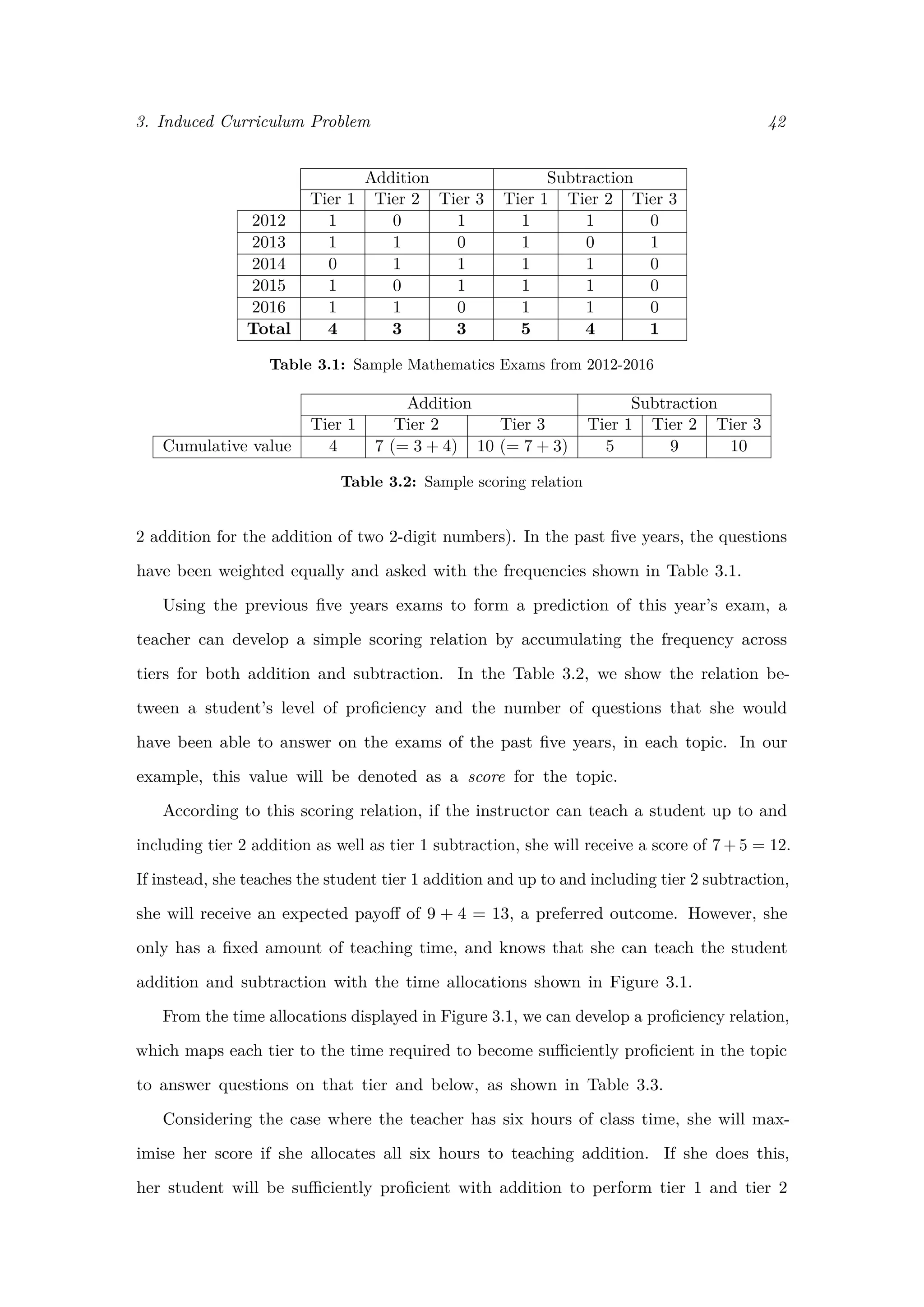
3.1 Sample teaching progression . . . . . . . . . . . . . . . . . . . . . . . . . . 43
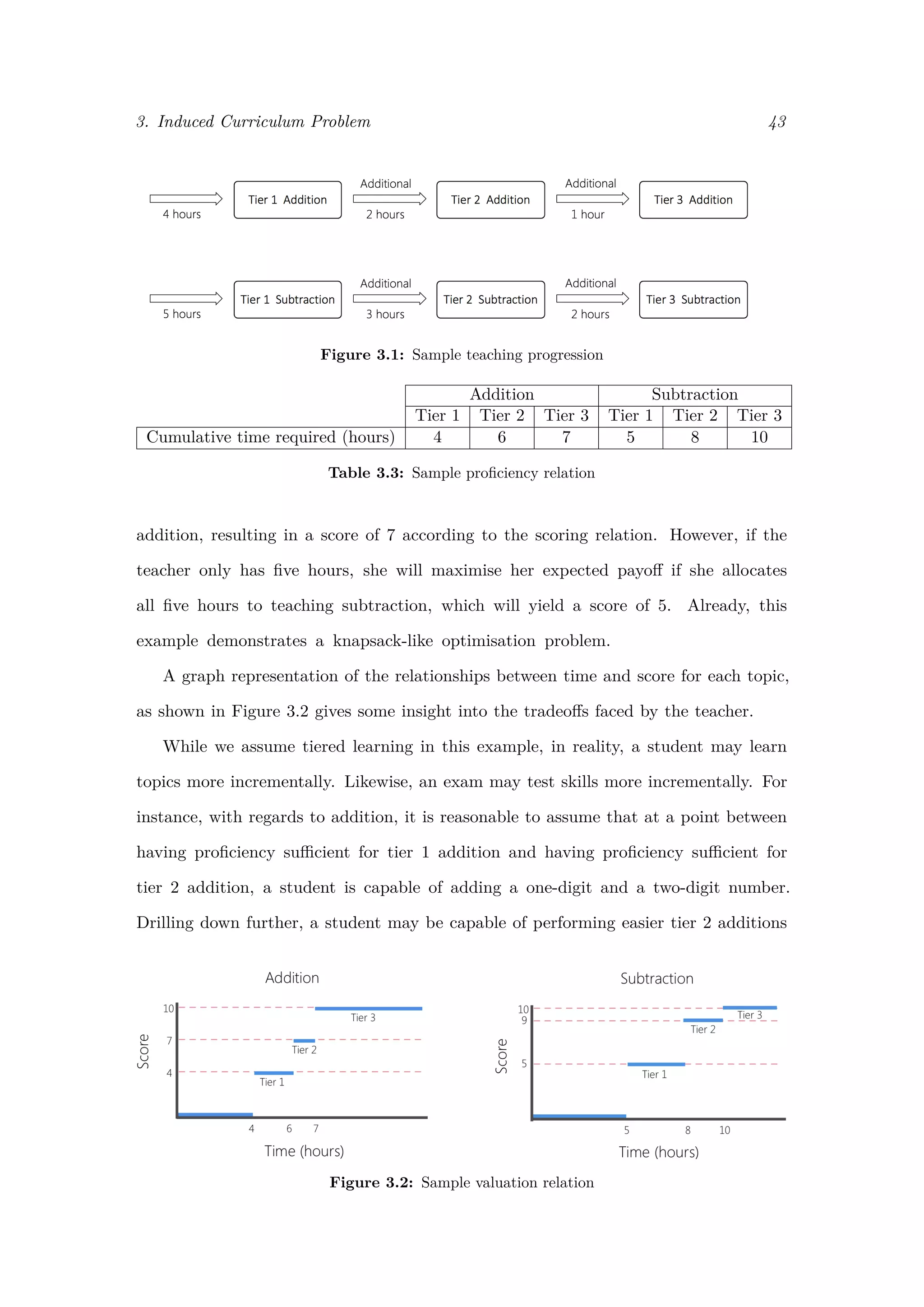
3.2 Sample valuation relation . . . . . . . . . . . . . . . . . . . . . . . . . . . 43
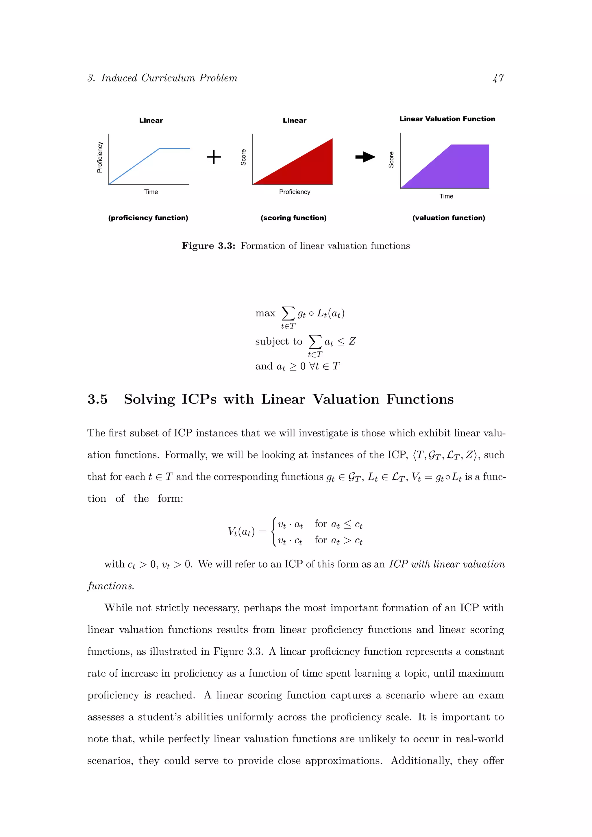
3.3 Formation of linear valuation functions . . . . . . . . . . . . . . . . . . . . 47
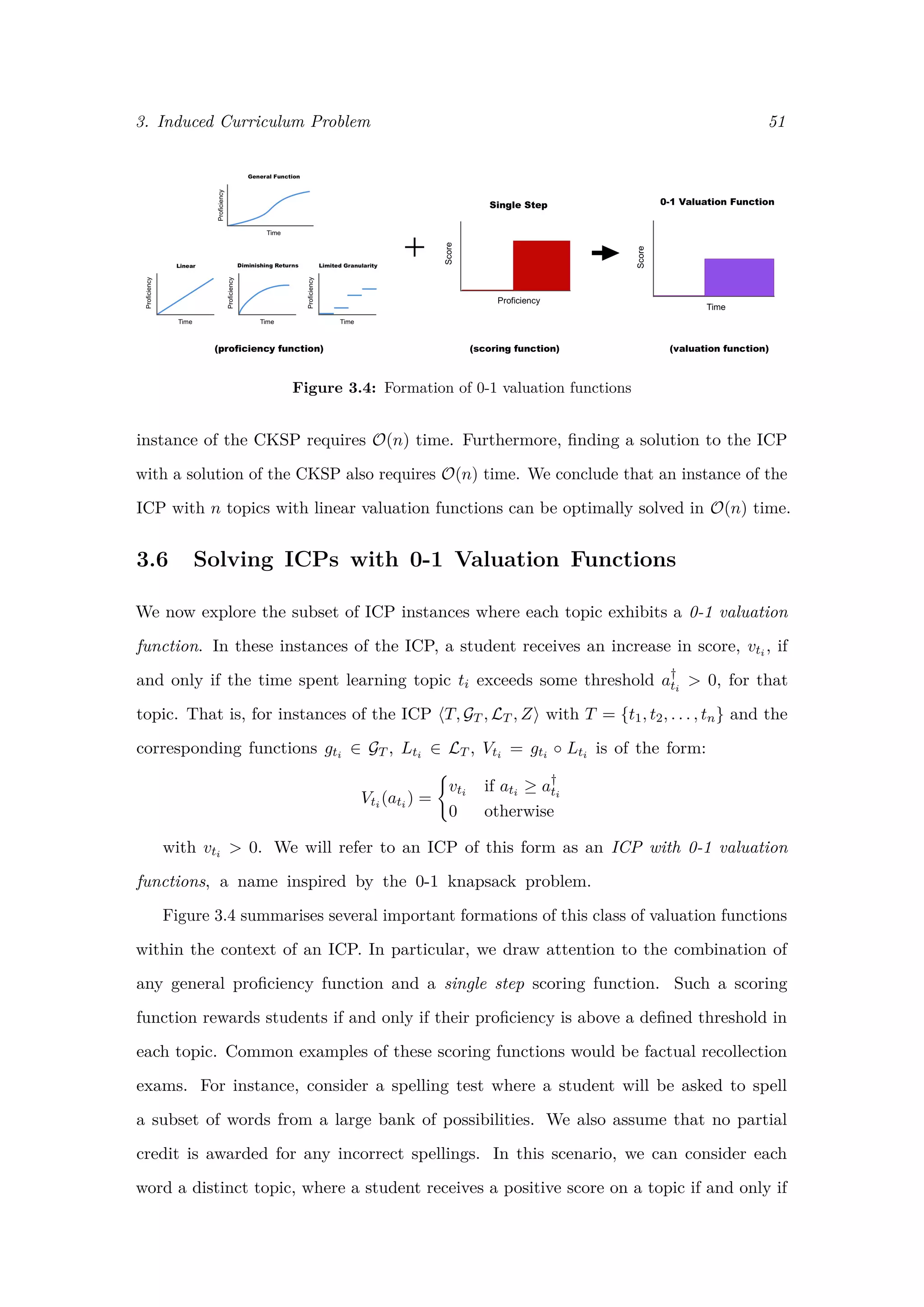
3.4 Formation of 0-1 valuation functions . . . . . . . . . . . . . . . . . . . . . 51
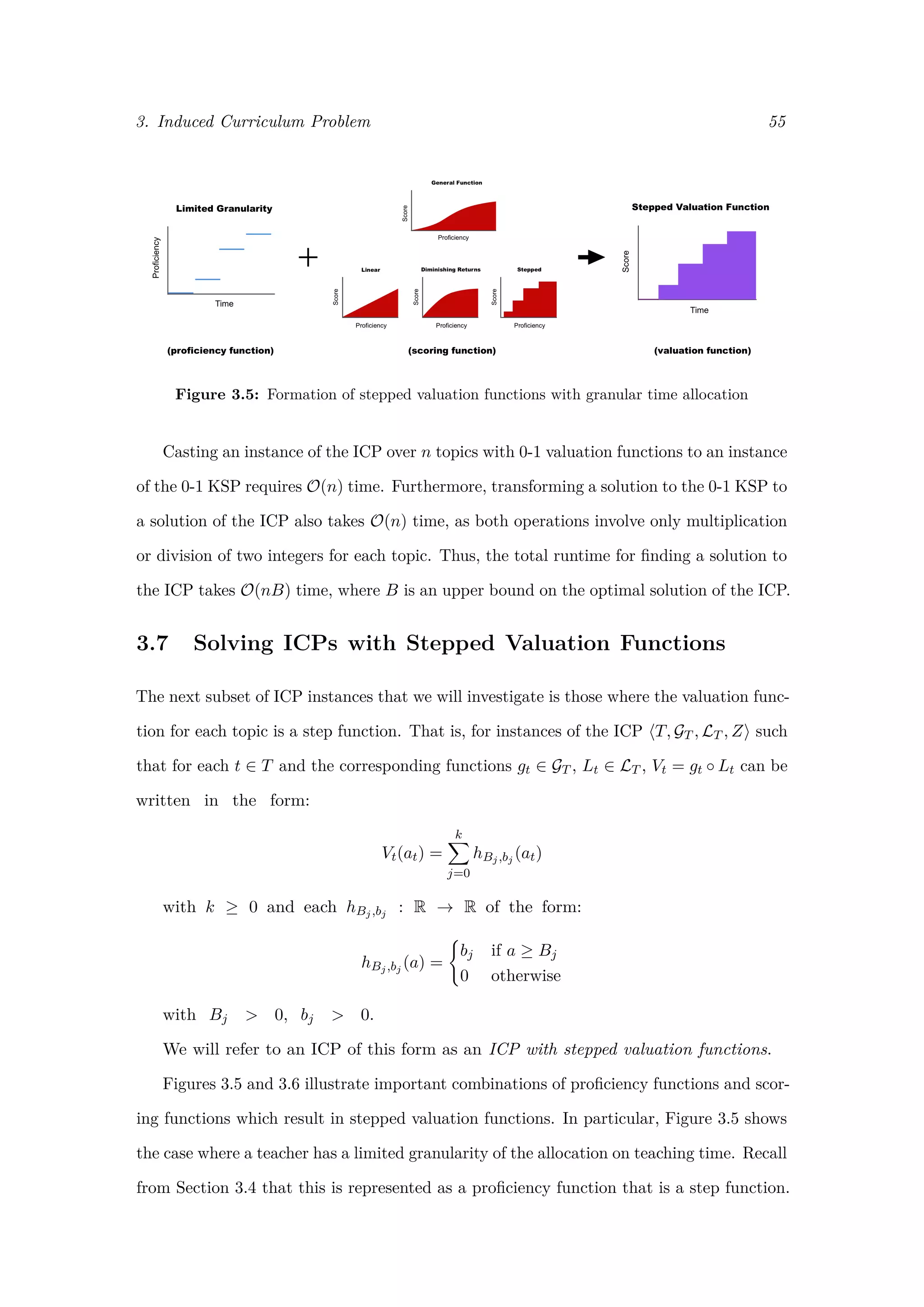
3.5 Formation of stepped valuation functions with granular time allocation . . 55
3.6 Formation of stepped valuation functions with stepped scoring . . . . . . 56
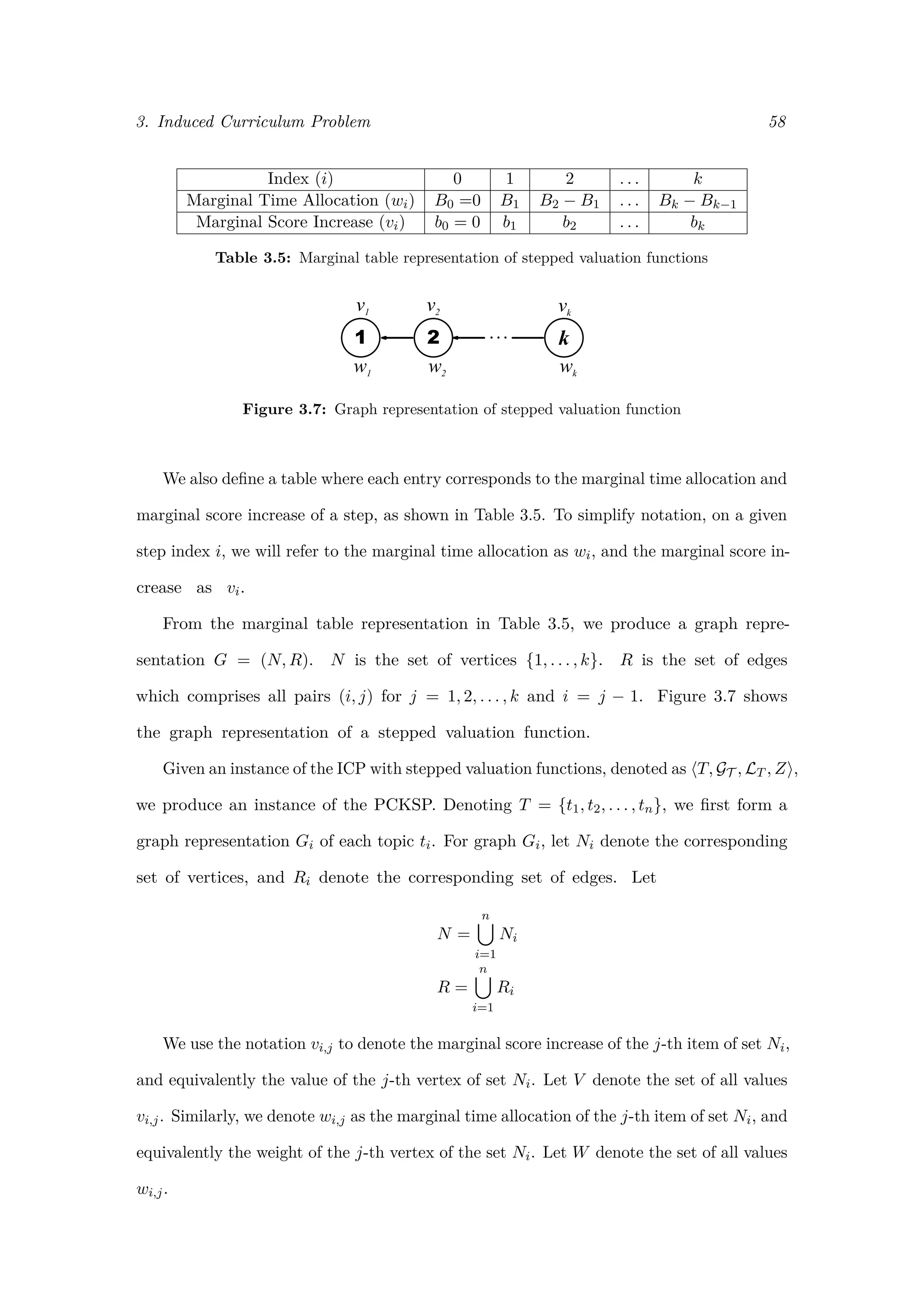
3.7 Graph representation of stepped valuation function . . . . . . . . . . . . . 58
3.8 Separate, stacked, and tree topic structures . . . . . . . . . . . . . . . . . 62
3.9 Splitting a topic structure . . . . . . . . . . . . . . . . . . . . . . . . . . . 65
3.10 Generating PCKSP from stepped valuation functions over unit connected
topic structures . . . . . . . . . . . . . . . . . . . . . . . . . . . . . . . . . 66
vi

7. 1Introduction
8.A.8 Multiply a binomial by a monomial or a binomial (integer coefficients)
8.A.11 Factor a trinomial in the form ax2 + bx + c; a = 1 and c having no more than three
sets of factors
In 2006, the New York State Department of Education listed these two items un-
der the “Algebra Strand” of the Grade 8 mathematics standards [1]. The standards
made no indication of relative importance, nor any recommendation on how much
time should be allocated to teaching each item. In the first four years after the
release of these standards, the first item was tested six times in the annual state
issued examination. The second item was not tested at all.
In 2007, the same New York State Department of Education initiated a program
which offered $3,000 per union teacher to schools which were able to meet goals of student
achievement, measured according to state issued examinations [2]. With this, the situation
in New York created a setting ripe for a practice known as teaching to the test.
Of course, the pairing of predictable state issued examinations and state issued
incentives (or accountability measures) is not one that is at all unique to New York.
Across the globe, the rise of high-stakes testing has placed considerable pressure not
only on students, but also on teachers and school administrators. As a result, recent
years have witnessed growing evidence of teaching to the test [3].
1

8. 1. Introduction 2
While case-based evidence is essential for diagnosing and monitoring this phenomenon,
it is typically costly and can, at times, be detrimental to the natural flow of the education
process. Our research aims to create models which embody the globally present interaction
between examination writers and teachers. To achieve this, we leverage two well-studied
mathematical problems: the Stackelberg Security Game and the knapsack problem.
In Chapter 2, we use Stackelberg Security Games (SSGs) to model the challenge faced
by examination writers in creating tests which are intended to assess student proficiency
across a full gamut of curriculum topics with only a limited number of questions. Since
2008, SSGs have established themselves as a powerful framework for generating security
strategies that have been implemented, with great success, by agencies including the US
Coast Guard and Federal Air Marshal Service [4, 5]. In our model, teachers use previous
exams to predict which topics will not be covered on the test, allowing these topics to be
removed from the class curriculum. The examination writer, on the other hand, must
create a test which is unpredictable, yet takes into account the relative importance of
topics. We create a model enabling us to cast this scenario to a Stackelberg Security
Game. Additionally, we present the first publicly available solver for SSGs, and provide
a novel analysis on the robustness of the model to uncertain inputs.
In Chapter 3, we formulate a problem whose solution is intended to quantify the effect
of teaching to the test on classroom curricula. Assuming that the teacher has knowledge
of what material will be tested, we use generalisations of the knapsack problem to find the
optimal allocation of class time amongst the set of curriculum topics. The solution to our
proposed problem maximises student exam scores, taking into account student learning
curves and exam content, simulating an instructor who perfectly teaches to the test. To al-
low for modeling of more complex scenarios, we introduce the notions of question difficulty,
prerequisite topics, and different student types who all exhibit distinct learning curves.
In this introductory chapter, we present the motivation behind our analysis. We
describe the role of assessments in education systems and how they are used to provide
measures of school and teacher accountability. We present evidence of the pressure which
high-stakes testing places on teachers, and discuss several means of gaming the system used
to boost examination scores. In particular, we focus on a form of gaming the system which

9. 1. Introduction 3
we refer to as teaching to the test, explaining the characteristics of exams which make it an
effective method. Finally, we claim that, despite its weighty consequences, the extent and
effect of teaching to the test remains a relatively unexplored topic due to a lack of research.
It is important to note that we do not adopt any stance on the presence of high-
stakes testing in education systems. We simply claim that teaching to the test is
a widely documented occurrence, and aim only to give insight regarding two man-
ners: (i) on the creation of exams which minimise the consequences of teachers re-
moving items from class curricula; and (ii) on the effects of exams on reallocating
class time to focus on topics that are more likely to be tested.
1.1 Terminology
While the terminology used to discuss testing will already be familiar to readers, we
provide the following definitions to ensure clarity throughout this chapter:
• We refer to a student as a person whose knowledge of a subject will be assessed by
a test. While we mainly focus on traditional classroom settings, keep in mind that
some of our discussion and analysis is applicable to other settings, such as online
courses.
• We refer to a teacher as a person who is instructing one to many students on a
subject.
• We refer to a subject as the branch of study which a student is learning. A subject
is made up of related topics.
• We refer to a topic as a contained element of a course. An exam question will
typically focus on just one topic.
• We refer to an assessment as any means of measuring a student’s attainment in a
subject. Assessments are not necessarily written tests.
• We refer to a test as a written assessment. The term examination (exam) also refers
to a written assessment, but is traditionally used when referring to end-of-course
written assessments. We attempt to maintain this pattern.

10. 1. Introduction 4
1.2 The Role of Assessments
The primary purpose of assessments is to provide an accurate measure of student
attainment. Assessments in the form of written exams are a particularly cheap and
efficient attempt at fulfilling this purpose. While exams importantly provide feedback
to both students and teachers on learning progress, the impact of test scores can reach
far beyond classroom walls. With specific regard to national exams, David Bell, former
Permanent Secretary at the Department for Children, Schools and Families (DCSF), states:
We want [national exams] to provide objective, reliable information about
every child and young person’s progress. We want them to enable parents to
make reliable and informative judgements about the quality of schools and
colleges. We want to use them at the national level, both to assist and identify
where to put our support, and also, we use them to identify the state of the
system and how things are moving [3].
Drawing from Bell’s statement and a 2008 report released by the Children, Schools, and
Families Committee [3], we assemble a non-exhaustive list of usages of test results within
the UK:
1. Student qualification. Standardised testing provides a means of ranking students
across the nation. Results can be considered (non-exhaustively) in (i) diagnosing
learning difficulties and need for intervention and special resources; (ii) determining
a student’s readiness to move on to the next level of education; and (iii) measuring
a student’s qualification for a vocational position.
2. Teacher and school accountability. Student test scores are accumulated and
used to provide standardised indicators for class and school performance. These
results give insight into which schools require government interaction due to poor
performance.
3. Performance tables. Each year the UK Department of Education uses national
test results to publish data on student attainment. These league tables are widely
used by parents to compare and select schools for their children.
While the merit of using a single national test to simultaneously serve as a multi-
objective indicator has been questioned [3], the current state of affairs in the UK

11. 1. Introduction 5
routinely witnesses national tests which providing input into all three of the above
objectives. This procedure, which is certainly not unique to the UK, results in test
scores which are impactful on individual, local, and national levels.
1.3 Gaming the System
The term high-stakes testing is used to capture the weighty consequences of test scores,
generally with reference to nationally-administered standardised exams. While pressure
on students likely comes as no surprise, the accountability procedures, as described above,
place comparable pressure on teachers. In a 2015 survey [6], a UK teacher explains :
[In my previous school] there was an inordinate amount of pressure put on
teachers to ensure that students achieved their target grades.
As a result of the high stakes faced by students and teachers alike, instructors have
turned to exam-specific methodologies for improving test scores.
1.3.1 Various Forms of Gaming the System
While exams are intended to provide an accurate measure of student attainment, they
undoubtedly cause unwanted side effects in the form of distorted curricula, time spent
reviewing marking rubrics, and turning to revision guides instead of textbooks. We
refer to gaming the system as an examination-specific practice which intends to im-
prove test results without achieving an overall greater understanding of course ma-
terial for the student (a definition inspired by [3, 6, 7]).
While some strategies for gaming the system exhibit a clearly dubious ethical nature,
Dr. Michelle Meadows, of the University of Oxford, explains that other methods
find themselves in a grey zone of questionable conduct, whose effects on education
are difficult to gauge. Drawing from Meadows’ report [8] and an additional report
by Jennifer Jennings and Jonathan Bearak, of New York University [9], we compile
a non-exhaustive list of strategies for gaming the system:
1. Explicit cheating: This encapsulates any clear unethical behaviour on the part
of the teacher or student. For example, a administering a test can change students’
answers after collection or give out hints during the exam.

12. 1. Introduction 6
2. School-wide decisions: With full knowledge of the consequences of poor national
test scores, schools may consider switching to easier exam boards or making changes
to which exam subjects they offer [8, 9].
3. Test Coaching: This covers a range of strategies from familiarising students with
test formats to providing students with frameworks to use during the standardised
exams [8].
4. Teaching to the test: While its usage varies across literature, we define teaching
to the test as an intentional modification of curriculum with the sole intent of
improving test scores based on the topics which are more likely to appear on the
test.
This research focuses specifically on the last mentioned strategy of gaming the system:
teaching to the test.
1.4 Teaching to the Test
All things considered, teaching to the test is widely viewed as an effective means of
raising test scores [3, 6, 7, 9]. The primary cause of its effectiveness is the predictability
of exams. Spark Notes LLC, a leading provider in test preparation material, makes
this statement about the SAT II Biology exam, a national standardised test whose
results are used to determine a student’s university readiness:
The SAT II Biology test has some redeeming qualities. One of them is
reliability. The test doesn’t change much from year to year. While individual
questions will never repeat from test to test, the topics that are covered and
the way in which they’re covered will remain constant.
Daniel Koretz of the Harvard Graduate School of Education, attributes the predictabil-
ity of exams to two main factors, summarised below [10]:
1. The challenge faced in forming questions of a desired difficulty level which accurately
assess student understanding. Exam questions which proved to give an accurate
measure of student attainment in previous years serve as excellent models for quickly
and cheaply writing new questions [10].

13. 1. Introduction 7
Figure 1.1: Case study provided by Jennings and Bearak [9]
2. The desire for consistent test difficulty across years. Failure to meet this requirement
has resulted in protests from students, teachers, and parents in the past [10].
Creating exams is an exercise in sampling. Due to time constraints, it is not possible
to cover all curriculum topics on an exam. Furthermore, any randomisation of test
material must take into account the relative importance of different topics, and the
need to keep some notion of similarity between exam iterations.
A report from Jennings and Bearak [9] provides a comprehensive study of topic
coverage on US standardised exams across three states over four years. In particular,
this study serves to prove the substantial advantage that can be gained by teaching to
the test. Table 1.1 shows their results, as presented in the original study [9]:
In New York ELA exams and New York and Massachusetts mathematics exams over
the four years spanning 2006 to 2009, less than two-thirds of all standards appeared on
any assessment. By eliminating these untested standards from class curricula, instructors
can allocate more time to teaching standards which are more likely to be tested. We
refer to this as narrowing the curriculum, where teaching to the test sacrifices breadth
of learning for depth of learning, focusing on topics that are more likely to appear
on exams. This type of teaching to the test is investigated in depth in Chapter
2. In general, however, teaching to the test can result in many forms of distorted
curricula. This more general consequence is studied in Chapter 3.

14. 1. Introduction 8
1.5 Our Contributions
A 2008 report released by the Children, Schools, and Families Committee of the UK
House of Commons made the following statement on teaching to the test [3]:
We recommend that the Government reconsiders the evidence on teaching
to the test and that it commissions systematic and wide-ranging research to
discover the nature and full extent of the problem.
A proper system for education needs little in the way of an introduction regarding its
benefits worldwide. Teaching to the test is a practice which introduces an unknown
factor into education systems, jeopardising its effectiveness. The House of Commons
report reiterates the need to better understand its implications.
The research that we present takes two very distinct, but well-studied mathematical
problems, and applies them both within the context of student assessments with the
goal of providing insight into the growing problem of teaching to the test.
Examination Security Game
In Chapter 2, we introduce the Examination Security Game (ESG), which models the
interaction between an examiner and a teacher as a Stackelberg Security Game (SSG). In
traditional applications, SSGs model the interaction between an attacker and a defender.
The defender wishes to optimally allocate a limited number of security resources across
a set targets, each of which has a distinct value. The attacker, on the other hand,
can observe the defender’s strategy and plan her attack accordingly. The attacker also
has her own set of target values, distinct from those of the defender. Knowing that
the attacker has full observational capabilities, the defender must develop a security
strategy which is unpredictable, yet still accounts for target values. SSGs have been
implemented with great success in a range of applications facing this challenge [4, 5,
11–15], speaking to their ability to contribute in real-world scenarios.
The development of our ESG model serves as a major contribution of this chapter.
In particular, we show that the same critical assumptions of an SSG hold within the
examiner-teacher setting. Notably, the examiner plays the role of the defender and must
use a limited number of exam questions to cover a large bank of topics. The teacher,

15. 1. Introduction 9
on the other hand, plays the role of the attacker, using past exams to predict which
topics will be tested. Claiming that critical assumptions of an SSG hold, we further assert
that the solution to the Examination Security Game yields an optimised strategy for
creating unpredictable exams which minimise the effects of teaching to the test.
Secondly, we implement an algorithm for solving SSGs that was proposed by Kiek-
intveld et al. [16]. We provide an implementation in Mathematica which is used in our
experimental analysis. Additionally, we provide an implementation coded in JavaScript.
To the best of our knowledge, no solver for the SSG has previously been made publicly
available. Furthermore, research within recent literature often makes use of IBM’s
CPLEX studio, a costly optimisation software product. Because of the incredible range
of applications of SSGs, we wanted to provide a more accessible alternative to using
an expensive solver. Our JavaScript implementation serves this purpose.
Finally, we present and analyse the results from a number of experiments. Notably,
we present novel analysis on the robustness of SSGs under the assumption of uncertain
inputs. We leverage cosine similarity as a metric of similarity between SSG solutions,
and provide extensive analysis on the sensitivity of the model to changes in input.
Our analysis suggests that small changes in target values typically provoke small to
moderate changes in solutions. However, we found that a small change in the number
of available resources leads to a much larger changes in solutions. These results suggest
that exam creation is a difficult and sometimes counter-intuitive problem, and that
SSGs offer a fairly robust framework for providing solutions.
Induced Curriculum Problem
In Chapter 3, we pose the Induced Curriculum Problem (ICP). While we take the viewpoint
of the examiner in formulating the ESG, we switch our perspective to that of the teacher
in formulating the ICP. In short, this problem embodies a scenario where a teacher is
attempting to optimally teach to the test. In finding this optimal teacher strategy, we
intend to gain insight into how an exam’s subject matter influences class curricula.
Again, our model development is a major contribution within this chapter. The
challenge faced by teachers is a direct result of a limited amount of teaching time. Simply

16. 1. Introduction 10
put, there is not sufficient time to achieve student mastery across all topics. As a result,
allocating class time becomes an optimisation problem. The knapsack problem describes
a similar optimisation problem, where the goal is to maximise the total value of objects in
a knapsack which has a limited capacity. We cannot fit all items in the knapsack, so we
must choose an optimal subset of the items, based on their individual values and weights.
Unfortunately, optimising the allocation of class time across topics is a much more
complex problem than the standard knapsack problem. We formulate the ICP tak-
ing into account several factors which influence the relationship between allocation
of class time and exam scores. First, we account for a range of difficulty of exam
questions. That is, a student may have sufficient proficiency in a topic to answer
easier questions, but is unable to answer more difficult questions. We take into account
different distributions of questions on exams by introducing scoring functions, which
map a level of student proficiency in a topic to a score. Because each topic exhibits
its own learning curve, we also introduce proficiency functions, which map the amount
of time spent teaching a topic to a level of proficiency in that topic.
Our analysis involves solving instances of the ICP whose proficiency functions and scor-
ing functions exhibit special features, which one would expect within the context of exami-
nations. Within each instance, we leverage a generalisation of the knapsack problem to find
an optimal solution. For example, the precedence constrained knapsack problem (PCKSP)
serves as an excellent model for solving instances of the ICP with stepped scoring functions,
where students are rewarded incrementally as their proficiency surpasses defined thresholds.
The PCKSP is also used in solving instances of the ICP which exhibit complex topic
structures. In these instances, we assume that learning one topic may first require learning
a prerequisite topic. This relationship has very natural mappings to the PCKSP, where
some items can only be placed in the knapsack on the condition that a distinct item is also
placed in the knapsack. However, as we will discuss, in complex prerequisite relationships,
we may first need to split the topic structure in order to leverage the PCKSP.
Finally, we introduce student types. In most scenarios, an instructor will be teaching
a class full of students who all have different abilities. We account for this by introducing
a set of distinct proficiency functions into the optimisation problem. With this, we

17. 1. Introduction 11
also discuss different notions of social welfare within the ICP, exhibited as different
optimisation objectives. Under the assumption of different student types, the notion of
optimality becomes nontrivial. For instance, while one teacher may wish to maximise the
sum of all students’ exam scores, another may wish to maximise the number of students
who score above a certain threshold. In the larger context, different objective functions
allow the ICP to capture different accountability pressures placed on teachers.

18. 2Examination Security Game
Contents
2.1 Introduction . . . . . . . . . . . . . . . . . . . . . . . . . . . . . 12
2.2 Stackelberg Security Games: A Case Study . . . . . . . . . . 14
2.2.1 Characteristics of SSGs . . . . . . . . . . . . . . . . . . . . . . . 15
2.2.2 Stackelberg Security Games . . . . . . . . . . . . . . . . . . . . . 17
2.3 Examination Security Game: Developing the Model . . . . . 20
2.3.1 Fulfilling the Assumptions of SSGs . . . . . . . . . . . . . . . . . 21
2.3.2 Examination Security Game . . . . . . . . . . . . . . . . . . . . . 22
2.3.3 Efficiently Finding Strong Stackelberg Equilibriums . . . . . . . 25
2.4 Implementation of the ERASER Algorithm . . . . . . . . . . 28
2.4.1 Converting ERASER MILP to a Table of Linear Expressions . . 28
2.4.2 Solving ERASER MILP . . . . . . . . . . . . . . . . . . . . . . . 30
2.4.3 Results . . . . . . . . . . . . . . . . . . . . . . . . . . . . . . . . 31
2.5 Summary . . . . . . . . . . . . . . . . . . . . . . . . . . . . . . . 36
2.1 Introduction
Because of the scale of education systems, testing via written examinations continues to
be the primary means of evaluating student attainment. Due to time constraints, however,
exams have limits on the amount of material that can be tested. In general, it is not
possible to test students on all topics that are intended to be learned. By randomising
which topics are tested, instructors are incentivised to teach all topics which could possibly
appear on the exam. Still, examinations tend to prioritise items which are deemed more
important to learn. As a result, teachers who are faced with limited time and the pressure
12

19. 2. Examination Security Game 13
of high-stakes testing may narrow their curriculum by teaching only a subset of the
possible topics, based on what they believe will be tested. Extensive previous research
has, in fact, indicated the presence of teaching to the test in US and UK schools [6, 9,
17–19]. In particular, teachers are able to take advantage of access to previous exams and
accurately make predictions about which questions will appear on future exams.
The predictability of assessments is not a fault of the exam creators, but rather a
consequence of the limited length of tests. Exam creators are faced with the challenge
of producing an exam which yields an accurate measure of student attainment with
often far fewer questions than topics. Additionally, exam creators must take into account
the varying importance of each topic. As the number of topics increases, the shear
scale of the problem makes producing near-optimal exams very difficult for humans. In
an effort to provide a solution to this challenge and develop tests which minimise the
consequences of teachers narrowing curriculum, we introduce the Examination Security
Game (ESG) as an instance of a Stackelberg Security Game (SSG).
Within recent years, SSGs have established themselves as an effective framework for
developing optimised security strategies against a broad spectrum of physical security
threats. Since 2009, SSGs have been studied and implemented in settings including but
not limited to: (i) in-flight and airport security [4, 15]; (ii) for the US Coast Guard
across a number of select ports nationwide [5]; (iii) environmental protection [20]; (iv)
conservation efforts against poaching and illegal fishing [12]; and (v) urban security
in transit systems [14]. In each scenario, SSGs are used as a framework to generate
an optimal security schedule which randomly distributes a limited number of security
resources amongst a set of targets. The undoubtedly impressive track record of success
supports the use of SSGs to the challenge faced by exam boards in creating unpredictable
tests which cover a full gamut of topics with a limited number of questions.
In this chapter:
1. We model the interaction between examiners and teachers as a Stackelberg Security
Game. We demonstrate that the assumptions necessary for the SSG also hold
within our model. By leveraging the SSG framework, we aim to create exams which

20. 2. Examination Security Game 14
optimally use a limited number of questions to minimise the losses from teaching to
the test.
2. We implement a recently developed algorithm which uses mixed-integer linear
programming (MILP) to solve the optimisation problem faced in SSGs. We develop
an implementation in Mathematica for the purposes of experimentation, and develop
an implementation in the more popular JavaScript to serve as the first publicly
available solver for SSGs.
3. We perform a number of experiments to characterise the runtime of our solver
and introduce a novel approach for characterising the effect of uncertainty on the
outcome of SSGs.
Please note that we assume a basic knowledge of game theory. For a comprehensive guide
to the subject, please consider consulting the excellent text by Maschler et al. [21].
2.2 Stackelberg Security Games: A Case Study
To introduce Stackelberg Security Games, we present a setting where SSGs have been
successfully applied to generate security schedules for guarding against in-flight security
threats [4]. With this example, we aim to provide intuition to the format of SSGs before pre-
senting a formal description, and finally casting the problem of optimally randomising ex-
ams as an SSG.
In our case study, we consider the problem of deploying a limited number of air marshals
across commercial flights to protect against hijacking and other malicious attacks. There
are an estimated 30,000 flights in the United States every day, yet the Federal Air Marshal
Service (FAMS) has only an estimated 4,000 employed air marshals. To add to the
challenge, on any given day, only a portion of these air marshals are available for work [22].
In this scenario, FAMS must produce a security schedule, which allocates their limited
resources (air marshals) across the possible targets (flights). Furthermore, they must do so
under the assumption that potential attackers can employ surveillance tactics to monitor
previous security schedules before attacking. Certainly in this scenario, a deterministic
security schedule would present a security vulnerability, as a hijacker could simply attack

21. 2. Examination Security Game 15
a flight which would be unprotected according to the deterministic schedule. To combat
this, FAMS must introduce an element of randomness into the security schedule.
Taking nothing else into account, FAMS could present a security schedule which placed
air marshals across flights uniformly at random. Such a strategy would eliminate any
advantage an attacker could gain from performing surveillance, yet doing so would fail
to take into account the varying threat levels across different flights. Certainly, a flight
from Cincinnati to Albuquerque faces less of a threat than a flight from New York City
to Washington, DC. Intuitively, then, an air marshal should be present on the flight from
New York to Washington, DC with higher probability than the flight from Cincinnati
to Albuquerque. How, then, should FAMS create a schedule which is randomised, and
therefore unpredictable, but still takes into account varying threats?
2.2.1 Characteristics of SSGs
To solve the problem faced by FAMS, Milind Tambe et al. model the interaction as a
Stackelberg Security Game [4]. SSGs exhibit several key characteristics, which we will
briefly motivate here before providing formal definitions in Section 2.3.
Limited Resources to Protect Targets At their core, Stackelberg Security Games
model a scenario where a defender with limited resources is attempting to protect a set
of targets which face the threat of attack from an adversary. To do so, the defender
must commit to a security schedule, which represents a valid allocation of the available
resources across targets. In the above flight security example, an example of a valid
security schedule for a given day may entail deploying each available air marshal to
two flights. In this particular example, the schedule may also account for the current
location of air marshals as well as pairing flights based on the same arrival/departure
airport. Importantly, we make the assumption that a security schedule which covers all
targets is not feasible, thus creating a complex problem for security teams.
Leader-Follower Structure Critically, Stackelberg games are two-player games which
exhibit a leader-follower structure. This is an assumption of information asymmetry which
is based on the follower knowing the strategy of the leader. Specifically within the context

22. 2. Examination Security Game 16
NYC to Washington, DC Cincinnati to Albuquerque
Covered Uncovered Covered Uncovered
Defender Utility 5 -8 1 -2
Attacker Utility -8 9 -2 3
Table 2.1: Example utility values of an SSG
of SSGs, the leader is the defender, who first plays their strategy in the form of a security
schedule. The follower is the attacker, who plays an optimal response to the defender’s strat-
egy.
Covered v. Uncovered Targets SSGs account for two possible outcomes in the event
of an attack on a target. If the attacked target is uncovered (that is, if no defender
resource is deployed to the target at the time of attack), the attack is successful. This
results in a positive outcome for the attacker and a negative outcome for the defender.
If the attacked target is covered (that is, if a defender resource is deployed to the
target at the time of attack), the attack is unsuccessful. This results in a negative
outcome for the attacker and a positive outcome for the defender.
Variable Target Values As exhibited in the setting of deploying air marshals across
flights, the targets in SSGs face variable threats as a result of different risk/reward
payoffs to the attacker. The flight from New York to Washington, DC faces a higher
threat because hijacking this flight would provide more value to the attacker. In an SSG,
this value is captured by associating each target with a utility for the attacker in the
event of a successful or unsuccessful attack. These utilities vary from target to target,
embodying the risk/reward scenario faced by attackers. Likewise, for each target, the
defender receives utility payoffs which represent the loss or gain of a successful or thwarted
attack on that target. To illustrate this notion, Table 2.1 presents sample utility values
for flights from NYC to Washington, DC and from Cincinnati to Albuquerque.
The challenge of allocating scarce resources across many targets is not unique to
aircraft security. The above security problem has been studied within the context of port
protection [5], wildlife conservation [12], and airport security [11, 15]. Computational
game theory offers a framework for modeling these problems and the computational

23. 2. Examination Security Game 17
engine for creating a randomised security schedule which maximises the capabilities of
a limited set of resources. In the following section, we formally present SSGs.
2.2.2 Stackelberg Security Games
With some intuition to the model and purpose of SSGs, we now more make a more formal
presentation, adapting notation found throughout the literature [4, 16, 23, 24].
Definitions and Notations
A Stackelberg Security Game, coined originally by Kiekintveld et al. in 2009 [16], is a
two-player game between a defender, D, and an attacker, A. The defender is tasked
with protecting a target set of size n using a resource set of size m. The target set is
denoted T = {t1, t2, . . . , tn}, and the resource set is denoted R = {r1, r2, . . . , rm}.
A set of schedules is denoted as S ∈ 2T , where each schedule s ∈ S represents a
set of targets that can be simultaneously defended by one resource. An assignment
function A : R → 2S, indicates the set of schedules which can be defended by each
resource. That is, ri can cover any schedule s ∈ A(ri) [16, 23].
The attacker’s pure strategy space, denoted by A, is the set of targets. A mixed strategy
for the attacker over these pure strategies is represented by a vector a = a1, a2, . . . , an ,
where each ai denotes the probability of attacking target ti.
The defender’s pure strategy space, denoted by D, is the set of feasible assignments
of resources to schedules. That is, each resource ri is assigned to a schedule si ∈ A(ri).
Critically, SSGs make the assumption that covering a target with one resource provides
the same protection as covering it with multiple targets. The defender’s pure strategy
can be represented by a coverage vector d = d1, d2, . . . , dn . Each component di ∈ {0, 1}
denotes the whether target ti is covered (di = 1) or uncovered (di = 0). A mixed strategy
for the defender, C, is a vector which specifies the probabilities of playing each d ∈ D.
Cd
denotes the probability of deploying the feasible coverage vector d. Additionally, let
c = c1, c2, . . . , cn be the vector of coverage probabilities corresponding to C such that each
component ci = d∈D
diCd
, a sum representing the marginal probability of covering ti [23].

24. 2. Examination Security Game 18
Utilities
As expressed in Table 2.1, the payoffs to each player in the event of an attack depend
only on whether or not the attacked target was covered by some defender resource. This
critical feature allows us to sufficiently define payoffs over an entire SSG by defining
four payoffs for each target: a utility for the defender and for the attacker in the event
target ti was attacked in the cases that it was covered or uncovered.
• Uu
A(ti) denotes the attacker’s utility for attacking target ti when it is uncovered.
That is, when no defense resource is allocated to ti.
• Uc
A(ti) denotes the attacker’s utility for attacking target ti when it is covered. That
is, when there is some defense resource allocated to ti.
• Uu
D(ti) denotes the defender’s utility in the event of an attack on target ti when it
is uncovered.
• Uc
D(ti) denotes the defender’s utility in the event of an attack on target ti when it
is covered.
Expected Utility
The expected utility for both players is dependent upon these utilities and the strategy
profile C, a . For a given defender strategy C, we denote the attacker’s expected
utility from attacking ti as UA(C, ti). Recalling that ci, calculated from C, denotes the
probability that the defender allocates a resource to cover ti, it follows that:
UA(C, ti) = ci · Uc
A(ti) + (1 − ci) · Uu
A(ti)
[25]
Summing over all targets weighted by the probability of an attack on each, as indicated
by the attacker’s mixed strategy a, we conclude that the expected attacker utility, under
strategy profile C, a , is:
UA(C, a) =
n
i=1
ai · UA(C, ti)
=
n
i=1
ai (ci · Uc
A(ti) + (1 − ci) · Uu
A(ti))

25. 2. Examination Security Game 19
Likewise, we find the expected utility for the defender under strategy profile C, a :
UD(C, a) =
n
i=1
ai (ci · Uc
D(ti) + (1 − ci) · Uu
D(ti))
Strong Stackelberg Equilibrium
The solution concept which we are interested in is referred to as a Strong Stackelberg
Equilibrium (SSE). In short, this solution concept satisfies the property that the defender
will choose an optimal mixed strategy over their pure strategies based on the assumption
that the attacker will choose their optimal response to this defender strategy [16]. The
strong form of this equilibrium further assumes that, in the event the attacker has multiple
optimal responses, she will break the tie by choosing the response which yields maximum
expected utility for the leader. This assumption is justified due to the fact that, in the event
of a tie, the defender can prompt the SSE by playing a mixed strategy which is arbitrarily
close to the equilibrium, provoking the attacker to play the desired response [24]. Critically,
this assumption guarantees the existence of an optimal mixed strategy for the leader [26].
To formally define the requirements for an SSE, we first define the attacker’s response
function R(C), which maps a defender strategy to a set of optimal attacker responses to
that defender strategy. Additionally, we define r : C → R which maps a defender strategy
to the expected utility of an optimal attacker response. That is, r(C) = UA(C, x) where x ∈
R(C).
Definition 1. A strategy profile C, a forms a Strong Stackelberg Equilibrium if it
satisfies the following three conditions
1. The attacker plays an optimal response to the defender strategy:
UA(C, a) ≥ r(C)
2. The defender chooses an optimal mixed strategy based on the attacker’s response
function:
∀C , ∀y ∈ R(C ), ∃x ∈ R(C) s.t. UD(C, x) ≥ UD(C , y)

26. 2. Examination Security Game 20
3. The follower breaks ties optimally for the leader:
∀x ∈ R(C) U(C, a) ≥ UD(C, x))
[16, 23]
2.3 Examination Security Game: Developing the Model
Daniel Koretz, of the Harvard Graduate School of Education, provides a one-sentence
summary of a common problem of exams which we will be addressing:
The core of the problem is that the sampling from the target used in creating
most large-scale assessments is both sparse and predictable over time. [10]
In this section, we model the interaction between examiners and teachers1 as an Exami-
nation Security Game (ESG). ESGs are instances of SSGs which incorporate additional
assumptions to tailor the model to the setting. In particular, we will use ESGs to
investigate teaching to the test in the form of narrowing the curriculum, a strategy which
completely dismisses a topic, allocating no time to studying it. In the spirit of SSGs,
such behaviour will be referred to as attacking a topic. Optimally for a teacher, she
would predict exactly which topics will not be covered on the test and attack those
topics. To represent this notion within the context of ESGs, we reward a teacher with
a positive payoff when she can successfully predict a topic that will not appear on the
test. On the other hand, if a teacher attacks a topic which does appear on the test, she
will receive a negative payoff. Critically, the payoffs for the teacher are influenced by
the difficulty of the topic. If a teacher successfully attacks a more difficult topic, she
will save more time, and will accordingly receive a greater payoff in the ESG.
Meanwhile, an examiner aims to prevent teacher’s from successfully attacking topics.
If an examiner covers a topic which a teacher attacks, she receives a positive payoff. On the
other hand, if a teacher is attacks a topic which is not covered on the test, the examiner’s
1
Within ESGs, the term examiner refers to the person or group who determines what content will
appear on an exam. The term teacher refers to any person who decides how to allocate study time for a
student who will be taking the exam. By this definition, please keep in mind that the student may also
be her own teacher. For instance, this is the case for any self-initiated exam preparations, as well as in
self-taught and online courses.

27. 2. Examination Security Game 21
measure of student attainment is compromised, resulting in a negative payoff to the exam-
iner. Critically, the payoffs for the examiner are scaled based on the relative importance of
each topic.
Stackelberg Security Games make several key assumptions that formulate a realistic
model of physical security scenarios. In this section, we discuss the analogous assumptions
within a high-stakes testing setting, and demonstrate that the SSG model is fitting, in
some ways perhaps even more so than in its traditional security settings.
2.3.1 Fulfilling the Assumptions of SSGs
Leader-Follower Structure
As noted previously, SSGs exhibit a leader-follower model, an assumption of informational
asymmetry. Within traditional security settings, this assumption requires that an attacker
has the necessary means to obtain knowledge of the defender’s strategy, typically through
surveillance methods. In some security settings, such as air marshals defending against
hijacking, such surveillance would require extensive planning and substantial funding.
Within the context of test-taking, exam boards often make previous exams freely avail-
able [27–29]. Certainly, the necessary resources for obtaining knowledge of the examiner’s
testing strategy are marginal in comparison to most physical security settings. We conclude
that interaction between examiners and teachers fits very well into the leader-follower struc-
ture of Stackelberg games.
Limited Resources to Cover Many Topics
Within an SSG, a defender has a fixed number of resources that they can allocate to
cover targets. Analogously, within an ESG, we view each exam question as a resource
which the examiner allocates to topics according to their mixed strategy. The number
of exam questions is limited, meaning that not all possible topics can be covered on
an exam. Dr. Kimberly O’Malley, Pearson’s Senior Vice President for Research and
Development, has expressed the dilemma created by this setting:
Because we can’t test everything in a year (no one wants the test to be longer
than necessary), decisions must be made. [3]

28. 2. Examination Security Game 22
Variable Topic Values
To both the student and the examiner, utilities are topic-dependent. We assume that the
examiner is given some weighting of the importance of each topic. In the context of state
standardised tests, this weighting may be provided by the official state standards. In other
scenarios, the topic weighting may be provided by the examiners themselves. If a student
successfully attacks a topic, the examiner would prefer it be an attack on a topic which
has a smaller weight. This preference ranking is represented in the defender utilities.
On the other hand, a teacher will gain more time by eliminating a topic which
take 8 hours to teach in comparison to a topic which only takes 2 hours to teach.
In other words, a teacher would prefer to successfully attack more difficult topics.
This preference is expressed within the attacker utilities.
The fact that the examiner and teacher independently develop utilities for each topic
creates a complex interaction. In particular, we cannot make the assumption of a zero-sum
game.
2.3.2 Examination Security Game
In this section we formally introduce an Examination Security Game as an instance
of a Stackelberg Security Game. Due to the “security setting” of ESGs, we can make
several assumptions regarding the structure of exams which allow us to make mod-
ifications to our model to make the proceeding analysis more intuitive. In particu-
lar, we can remove the notion of assignment functions.
ESGs and Assignment Functions
Recall that, in the context of SSGs, an assignment function, A, indicates the set of
schedules that can be defended by each resource. From this assignment function, we
can generate a set of feasible coverage vectors, D, which allocate each resource ri to
some schedule s ∈ A(ri). The assignment function is introduced to handle complex
schedule feasibility challenges faced in real-world physical security domains, such as
the scheduling problem faced by FAMS with assigning air marshals to flights. In this
setting, each marshal can only be assigned to a very small subset of possible schedules

29. 2. Examination Security Game 23
due to their physical location and scheduled work hours. These constraints, however,
become superfluous within the context of the Examination Security Game.
Specifically, we assume that each exam question can cover any one single topic.
That is, if there are three questions on an exam (denoted Q1, Q2, and Q3), and five
potential topics, we assume that Q1, Q2, and Q3 could all cover any one of the five topics.
As with SSGs, we also assume that each question covers a unique topic, as covering
a target with multiple resources provides no benefit for the defender if that target is
attacked. 2 Following the notation of SSGs, the set of schedules within an Examination
Security Game is simply the set S = {s1, s2, . . . , sn} where si = {ti}.
With this in mind, assuming all that all m questions on the exam are used, the
set of possible pure strategies for the defender is set n
m .
Notation of ESG
The notation of the ESG very closely follows the notation of the SSG. The two players are
again denoted D and A. Keep in mind that, within the context of the ESG, D denotes
the examiner, and A denotes the teacher. The examiner must “protect” a set of n topics
T = {t1, t2, . . . , tn}. To do so, she has m questions at her disposal. Please note that,
following the above discussion, we no longer refer to the notion of a resource set.
The teacher’s pure strategy space, denoted by A, is the set of topics. A mixed strategy for
the teacher, denoted by a, is a vector where each component, ai, represents the probability
of attacking topic ti.
As discussed, the examiner’s pure strategy space, denoted by D, is the set of vectors
d ∈ n
m . A mixed strategy for the examiner is represented by a vector C = c1, c2, . . . , cn
with cidenoting the probability of covering topic ci. C must meet the following constraints:
1. The probability of each topic being on the exam is between 0 and 1:
ci ∈ [0, 1] for i = {1, 2, . . . , n}
2. The sum of all probabilities is at most m:
2
Both within the context of exams and physical security settings (e.g. in-flight security), it can be
argued that allocating multiple resources to a target offers some additional benefit to the defender. This
assumption is further addressed in Chapter 3. Within the SSG model, however, a target is only considered
in a “covered” or “uncovered” state.

30. 2. Examination Security Game 24
n
i=1
ci ≤ m
Once again, we refer to a pair C, a as a strategy profile.
An Example ESG
To clarify this model, we now provide a brief example.
Consider the simple example of an economics exam which could test students on the fol-
lowing four topics:
1. t1= Supply and demand
2. t2= Financial markets
3. t3= Government policy
4. t4= Foreign exchange
It follows that the target set T = {t1, t2, t3, t4}. The exam is a one hour essay based exam,
and because of the time constraint, allows only 2 of the 4 topics to be addressed (n = 4, m =
2).
It follows that there are 4
2 = 6 possible coverage vectors:
1. d1 = 1, 1, 0, 0
2. d2 = 1, 0, 1, 0
3. d3 = 1, 0, 0, 0
4. d4 = 0, 1, 1, 0
5. d5 = 0, 1, 0, 1
6. d6 = 0, 0, 1, 1
The set of feasible coverage vectors is D = {d1, d2, d3, d4, d5, d6}.
Considering the case that the examiner plays the mixed strategy C = 0.25, 0.25, 0, 0.25, 0.25, 0 .
The corresponding vector of coverage probabilities is c = 0.5, 0.75, 0.5, 0.25 , indicat-
ing the topics are covered with the following probabilities:
1. Supply and demand: 50%
2. Financial markets: 75%
3. Government policy: 50%
4. Foreign exchange: 25%

31. 2. Examination Security Game 25
Utilities in the ESG
For completeness, we denote the analogous player utilities within the context of the
ESG, and provide a summary of possible factors influencing their value.
• Uu
A(ti) denotes the teacher utility for attacking (i.e. not preparing for) exam target
ti when it is untested (uncovered)
• Uc
A(ti) denotes the teacher utility for attacking (i.e. not preparing for) exam target
ti when it is tested (covered)
• Uc
D(ti) denotes the examiner’s utility when the teacher attacks exam target ti and
it is tested (covered)
• Uu
D(ti) denotes the examiner’s utility when the teacher attacks exam target ti and
it is untested (uncovered)
Please note the expected utility functions for both players follow identically from those pre-
sented in Section 2.2.3.
2.3.3 Efficiently Finding Strong Stackelberg Equilibriums
In 2008, Kiekintveld et al. [16] introduced the ERASER (Efficient Randomised Allocation
of Security Resources) algorithm for efficiently finding SSEs of SSGs by casting the problem
as a mixed-integer linear programming (MILP) problem. ERASER leverages a concise rep-
resentation of a SSG which is realised through exploiting special characteristics of the game.
Concise Representation of SSGs
SSGs can be naively modeled with a normal-form representation which iterates over
all possible pure defender strategies. Given n targets and m resources, there are n
m
possible defender strategies, a value exponential in the number of topics. Because of this
exponential relation with respect to n, SSGs become unwieldy very quickly as the number
of targets grows if a normal-form representation is used. Table 2.2 presents an example
normal-form representation of pure strategies with n targets and m resources.
However, using the special features of SSGs, a compact representation has been
developed by Kiekintveld et al. [16], which we will use to efficiently find a solution to
ESGs. A critical characteristic of SSGs, and hence ESGs, is that player payoffs are

32. 2. Examination Security Game 26
Pure Strategy Index Covered Targets Probability
1 1,2 d1
2 1,3 d2
3 1,4 d3
4 2,3 d4
5 2,4 d5
6 3,4 d6
Table 2.2: Exponentially large iteration of pure strategies
Supply and Demand Financial Markets Government Policy Foreign Exchange
Covered Uncovered Covered Uncovered Covered Uncovered Covered Uncovered
Examiner 6 -1 9 -9 2 -3 7 -10
Student -6 5 -10 3 -7 4 -2 4
Table 2.3: Concise representation of utility
only dependent on the target attacked and whether or not that target is covered by
the defender. That is, within the context of ESGs, if a teacher attacks topic ti, the
resulting payoffs for both the examiner and the teacher are only dependent on whether a
question covering topic ti is on the exam. The payoffs are unaffected by whether or not a
question covering some topic tj, with tj = ti, is present on the test. This feature of SSGs
creates an additional structure which can be exploited to create a concise representation.
Exploiting this feature, Kiekintveld et al. [16] developed a concise representation of SSGs,
which we demonstrate in Table 2.3, continuing with the previous example::
ERASER Algorithm
The ERASER algorithm takes advantage of the concise representation of SSGs and
finds an optimal defender strategy in the form of a coverage vector. The ERASER
algorithm casts the SSG optimisation problem as a mixed-integer linear program (MILP).
We provide the MILP optimisation problem in equations 2.1 to 2.7, as presented by
Kiekintveld et al. [16], with only changes in notation:

33. 2. Examination Security Game 27
max d (2.1)
at ∈ {0, 1} ∀t ∈ T (2.2)
t∈T
at = 1 (2.3)
ct ∈ [0, 1] ∀t ∈ T (2.4)
t∈T
ct ≤ m (2.5)
d − UD(C, t) ≤ (1 − at) · Z ∀t ∈ T (2.6)
0 ≤ k − UA(C, t) ≤ (1 − at) · Z ∀t ∈ T (2.7)
The objective of the MILP, as presented in equation 2.1, is to maximise d, which
represents the examiner’s (defender’s) utility. Equations 2.2 and 2.3 require that the
attacker attacks just a single target with probability 1. This constraint simplifies the
computational requirements of finding a solution, yet is without any loss in generality as an
SSE still exists with this constraint applied. Specifically, the constraint listed in Equation
2.2 should generally be met by simply requiring the constraint in equation 2.3. Recalling
that the contribution of a single target t to the expected attacker utility is defined as
UA(C, a) = n
i=1 ai (ci · Uc
A(ti) + (1 − ci) · Uu
A(ti)), with ci, Uc
A(ti), and Uu
A(ti) all fixed
for i ∈ {1, 2, . . . , n}, we denote vi = (ci · Uc
A(ti) + (1 − ci) · Uu
A(ti)), and rewrite the at-
tacker’s expected utility
UD(C, a) =
n
i=1
ai · vi
with vi ∈ R for i ∈ {1, 2, . . . , n}. Under the constraint of Equation 2.2, it follows that
the attacker can maximize her expected utility by setting ai = 1 for the corresponding
maximum vi, and all other aj = 0 for i = j. However, in the case that vi = vj for
some i, j such that i = j, it is possible that the attacker maximizes her expected utility
otherwise, such as setting ai = aj = 0.5, and ak = 0 for all k which are not i or j.
Equation 2.2 is therefore necessary for allowing for computational simplifications.
Equation 2.4 ensures that the coverage vector is valid, constraining each element to a
valid probability in the interval [0, 1]. Equation 2.5 limits the defender’s coverage vector by
the amount of resources available, m.

34. 2. Examination Security Game 28
As explained by Kiekintveld et al. [16], Equation 2.6 introduces Z, a constant which
is larger than the maximum payoff for either the attacker or defender. To be sure, our
implementation sets Z to the product of the number of targets, n, and the maximum
utility for either player across all targets. Referring to the right hand side of Equation
2.6, the expression (1 − at) · Z evaluates to 0 for the attacked target, where at = 1, and
to Z for all other targets, where at = 0. As such, this constraint places an upper bound
UD(C, t) on d for only the attacked target. For unattacked targets, where at = 0, the
right hand side is equal to Z, and thus arbitrarily large. Because the MILP maximises d,
for all optimal solutions d = UD(C, a), it follows that C is maximal for any given a [16].
Equation 2.7 introduces a variable k. The first part of the equation forces k to be at
least as large as the maximal defender payoff received for an attack on any target. To make
the effect of the second part of the constraint more apparent, we can rewrite Equation 2.7:
0 ≤ k − ct · Uc
D(t) + (1 − ct) · Uu
D(t) ≤ (1 − at) · Z
For any target which is not attacked, such that at = 0, the constraint becomes:
0 ≤ k − ct · Uc
D(t) + (1 − ct) · Uu
D(t) ≤ 0
It follows that k−ct ·Uc
D(t)+(1−ct)·Uu
D(t) = 0 for any unattacked target. If the attack
vector specifies a target which is not maximal, this constraint is violated. The resulting
effect of the constraints placed by equations 2.6 and 2.7 ensure that the coverage vector,
C, and the attacking vector, a, are mutual best-responses in any solution which maximises d
[16].
2.4 Implementation of the ERASER Algorithm
2.4.1 Converting ERASER MILP to a Table of Linear Expressions
The ERASER algorithm was implemented in both Mathematica and JavaScript. To
utilise pre-existing MILP solvers, we first reformatted equations 2.1 to 2.7, writing them
as linear expressions over our list of variables from the ERASER MILP:
• d
• k

35. 2. Examination Security Game 29
• ct ∀t ∈ T
• at ∀t ∈ T
Recall that we are provided all utility values (Uu
A(t), Uc
A, Uu
D(t), and Uc
D(t)) for each topic
t ∈ T, as well as a large fixed constant Z. To ease the notational burden, we will
denote ∆D(t) = Uc
D(t) − Uu
D(t), and similarly ∆A(t) = Uc
A(t) − Uu
A(t).
The objective function is a simple linear function, as it aims to maximise d. Ad-
ditionally, the constraints introduced in equations 2.2 to 2.5 are already presented as
linear expressions over the set of variables. All that remains is reformatting equations 2.6
and 2.7 as linear expressions over our set of variables. Referring to the left-hand side of
Equation 2.6, and recalling that UD(t, C) = ct · Uc
D(t) + (1 − ct) · Uu
D(t), it follows:
d − UD(C, t) = d − (ct · Uc
D(t) + (1 − ct) · Uu
D(t))
= d − (ct (Uc
D(t) − Uu
D(t)) + Uu
D(t))
Now referring to the whole of Equation 2.6:
d − UD(C, t) ≤ (1 − at) · Z
d − (ct (Uc
D(t) − Uu
D(t)) + Uu
D(t)) ≤ (1 − at) · Z
d − ct∆D(t) + Z · at ≤ Z + Uu
D(t)
Noting that ∆D(t), Z, and Uu
D(t) are all constants, we conclude that we have written
our constraint as a linear equation of variables d, ct, and at.
Similarly, looking at the upper bound of Equation 2.7:
k − UA(C, t) ≤ (1 − at) · Z
k − (ct (Uc
A(t) − Uu
A(t)) + Uu
A(t)) ≤ (1 − at) · Z
k − ct∆A(t) + Z · at ≤ Z + Uu
A(t)
And finally, referring to the lower bound of Equation 2.7:
k − UA(C, t) ≥ 0
k − (ct (Uc
A(t) − Uu
A(t)) + Uu
A(t)) ≥ 0
k − ct∆A(t) ≥ Uu
A(t)
Combining the linear expressions of equations 2.2 to 2.7, we produce the complete table
of constraints, as presented in Table 2.4.

36. 2. Examination Security Game 30
d k c1 c2 . . . cn a1 a2 . . . an b
Eq. 2.2 for t1 0 0 0 0 . . . 0 1 0 . . . 0 ∈ {0, 1}
Eq.2.2 for t2 0 0 0 0 . . . 0 0 1 . . . 0 ∈ {0, 1}
. . . . . .
Eq.2.2 for tn 0 0 0 0 . . . 0 0 0 . . . 1 ∈ {0, 1}
Eq.2.3 0 0 0 0 . . . 0 1 1 . . . 1 = 1
Eq.2.4 for t1 0 0 1 0 . . . 0 0 0 . . . 0 ∈ [0, 1]
Eq.2.4 for t2 0 0 0 1 . . . 0 0 0 . . . 0 ∈ [0, 1]
. . . . . .
Eq.2.4 for tn 0 0 0 0 . . . 1 0 0 . . . 0 ∈ [0, 1]
Eq.2.5 0 0 1 1 . . . 1 0 0 . . . 0 ≤ m
Eq.2.6 for t1 1 0 −∆D(t1) 0 . . . 0 Z 0 . . . 0 ≤ Z + Uu
D(t1)
Eq.2.6 for t2 1 0 0 −∆D(t2) . . . 0 0 Z . . . 0 ≤ Z + Uu
D(t2)
. . . . . .
Eq.2.6 for tn 1 0 0 0 . . . −∆D(tn) 0 0 . . . Z ≤ Z + Uu
D(tn)
Eq. 2.7 for t1 0 1 −∆A(t1) 0 . . . 0 Z 0 . . . 0 ≤ Z + Uu
A(t1)
Eq. 2.7 for t2 0 1 0 −∆A(t2) . . . 0 0 Z . . . 0 ≤ Z + Uu
A(t2)
. . . . . .
Eq. 2.7 for tn 0 1 0 0 . . . −∆A(tn) 0 0 . . . Z ≤ Z + Uu
A(tn)
Eq. 2.7 for t1 0 1 −∆A(t1) 0 . . . 0 0 0 . . . 0 ≥ Uu
A(t1)
Eq. 2.7 for t2 0 1 0 −∆A(t2) . . . 0 0 0 . . . 0 ≥ Uu
A(t2)
. . . . . .
Eq. 2.7 for tn 0 1 0 0 . . . −∆A(tn) 0 0 0 ≥ Uu
A(tn)
Table 2.4: ERASER MILP represented as a table of linear expressions
Please note that constraints such as ci ∈ [0, 1] are handled by combining the
constraints ci ≤ 1 and ci ≥ 0. These were joined in the above table for brevity.
Likewise, constraints of the form ai ∈ {0, 1} are handled similarly, but also adding
the requirement that ai is an integer. In total, for an instance of ESG with n topics,
the corresponding MILP has 2n + 2 variables and 7n + 2 constraints.
2.4.2 Solving ERASER MILP
The ERASER algorithm casts the problem of finding a SSE to a MILP, taking advantage of
pre-existing MILP solvers to efficiently find a solution. In particular, the simplex method
and interior point methods are often used in practice for linear optimisation problems.
Simplex and revised simplex methods, while having a worst-case runtime exponential in
the number of constraints, and therefore in n in our case, typically perform much better
than worst case in practice. In fact, analysis by Spielman and Teng [30] demonstrates that
the simplex algorithm usually runs in polynomial time in the number of variables and
constraints. Furthermore, randomised simplex algorithms have been introduced which run
in worst-case polynomial time in the number of variables and constraints [31]. Interior point

37. 2. Examination Security Game 31
methods, on the other hand, allow for very fast machine-precision approximations, and
are an excellent option for large-scale MILPs [32]. Due to the relative uncertainty in these
methods, we provide runtime analysis on randomly generated instances of SSGs below.
JavaScript Implementation
Following the previous discussion, an implementation of ERASER coded in JavaScript was
developed as the first publicly available solver for SSGs. To solve the MILP, we leveraged
an open source JavaScript simplex algorithm [33]. The full code can be found in Appendix
A, and is also available at https://github.com/rcmoore38/stackelbergsecuritygamesolver.
Mathematica Implementation
A Mathematica implementation of ERASER was used to run experiments whose results are
found in the following section. This implementation takes advantage of Mathematica’s col-
lection of algorithms for solving linear optimisation problems. The full code can be found in
Appendix B.
2.4.3 Results
The following experiments were conducted on a 2.6 GHz Intel Core i5 3337U processor
with access to 8GB of RAM. All experiments were done running Mathematica 10.0,
using the built in function to solve the MILPs. This function uses a combination
of the revised simplex method and interior point methods.
Runtime Analysis
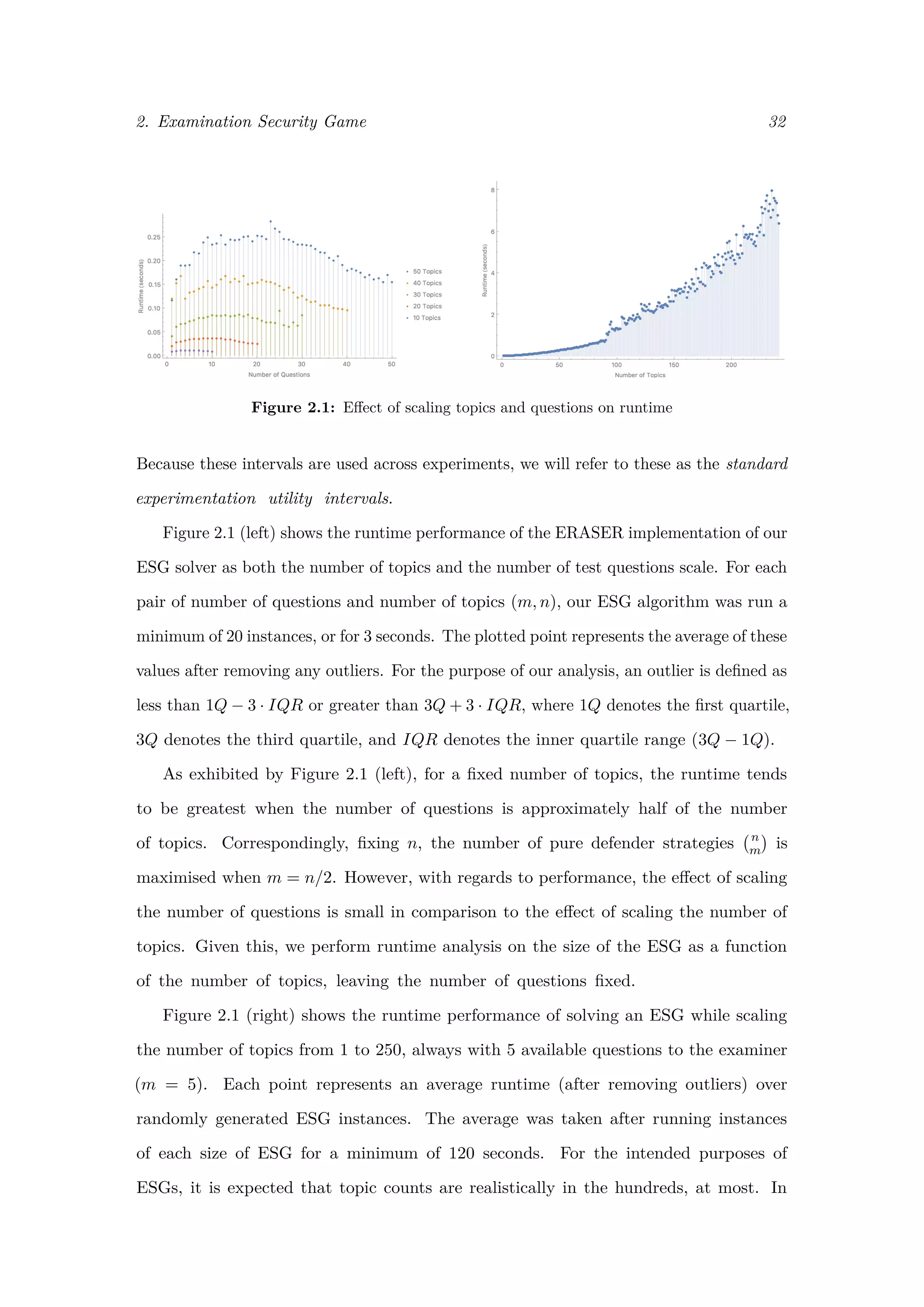
In the first set of experiments, we analyse the runtime of our algorithm on randomly
generated instances of ESGs, varying the number of topics and the number of exam
questions. For each instance, we randomly generate utility values, drawing indepen-
dently and uniformly at random from the following intervals:
• Uc
D(t) : [0, 10] ∀t ∈ T
• Uu
D(t) : [−10, 0] ∀t ∈ T
• Uc
A(t) : [−10, 0] ∀t ∈ T
• Uu
A(t) : [0, 10] ∀t ∈ T

38. 2. Examination Security Game 32
Figure 2.1: Effect of scaling topics and questions on runtime
Because these intervals are used across experiments, we will refer to these as the standard
experimentation utility intervals.
Figure 2.1 (left) shows the runtime performance of the ERASER implementation of our
ESG solver as both the number of topics and the number of test questions scale. For each
pair of number of questions and number of topics (m, n), our ESG algorithm was run a
minimum of 20 instances, or for 3 seconds. The plotted point represents the average of these
values after removing any outliers. For the purpose of our analysis, an outlier is defined as
less than 1Q − 3 · IQR or greater than 3Q + 3 · IQR, where 1Q denotes the first quartile,
3Q denotes the third quartile, and IQR denotes the inner quartile range (3Q − 1Q).
As exhibited by Figure 2.1 (left), for a fixed number of topics, the runtime tends
to be greatest when the number of questions is approximately half of the number
of topics. Correspondingly, fixing n, the number of pure defender strategies n
m is
maximised when m = n/2. However, with regards to performance, the effect of scaling
the number of questions is small in comparison to the effect of scaling the number of
topics. Given this, we perform runtime analysis on the size of the ESG as a function
of the number of topics, leaving the number of questions fixed.
Figure 2.1 (right) shows the runtime performance of solving an ESG while scaling
the number of topics from 1 to 250, always with 5 available questions to the examiner
(m = 5). Each point represents an average runtime (after removing outliers) over
randomly generated ESG instances. The average was taken after running instances
of each size of ESG for a minimum of 120 seconds. For the intended purposes of
ESGs, it is expected that topic counts are realistically in the hundreds, at most. In

39. 2. Examination Security Game 33
this range, the ERASER algorithm shows excellent performance. Please note that
the increase in variance after 80 topics is expected to be the result of Mathematica
switching from a simplex algorithm to an interior point method.
Robustness Analysis
Our game theoretic model assumes that the examiner has perfect knowledge of teacher’s
utilities for each topic. These utilities, according to our model, are inspired by the
amount of time that is needed to learn each topic. In this section, we investigate the
robustness of our model, under the premise that these utilities may not be perfect
representations. In particular, we look at the effect of varying teacher utility on the
SSE found the ERASER algorithm. Our analysis introduces a method which is novel
to the purpose of quantifying the difference of two SSEs: cosine similarity.
To measure the robustness of our model, we must first define a metric which provides
a meaningful measure of change between two solutions. Recall that the goal of ESGs is to
find a testing strategy which minimises the loss due to teacher’s gaming exams. Thus, to
create a meaningful metric for comparing two solutions, it would be beneficial to quantify
the difference between the defender’s coverage vector, which indicates the probability
that each question appears on the exam. To do this, we leverage cosine similarity.
To the best of our knowledge, there has been no prior study done within the context of
SSGs which analyses the effect of varying attacker utilities on the resulting solution cover-
age vector. Cosine similarity, due to its applications in data mining and measuring cohesion
within clusters, has become a widely used metric within the machine learning community.
In our experiments, we use it in two experiments which simulate an uncertainty in teacher
(attacker) utility, and compare the resulting coverage vectors using cosine similarity.
Before discussing results, we first explain the experiment methodology. For the
results shown in both charts of Figure 2.2, we use the same process of measuring
robustness. In short, we generate a random instance of the ESG and find an optimal
examiner strategy, represented as a coverage vector c. We then modify the input by
scaling the attacker utilities and find an optimal examiner strategy to this modified
problem, denoted c†. Using cosine similarity, we can then identify a relationship

40. 2. Examination Security Game 34
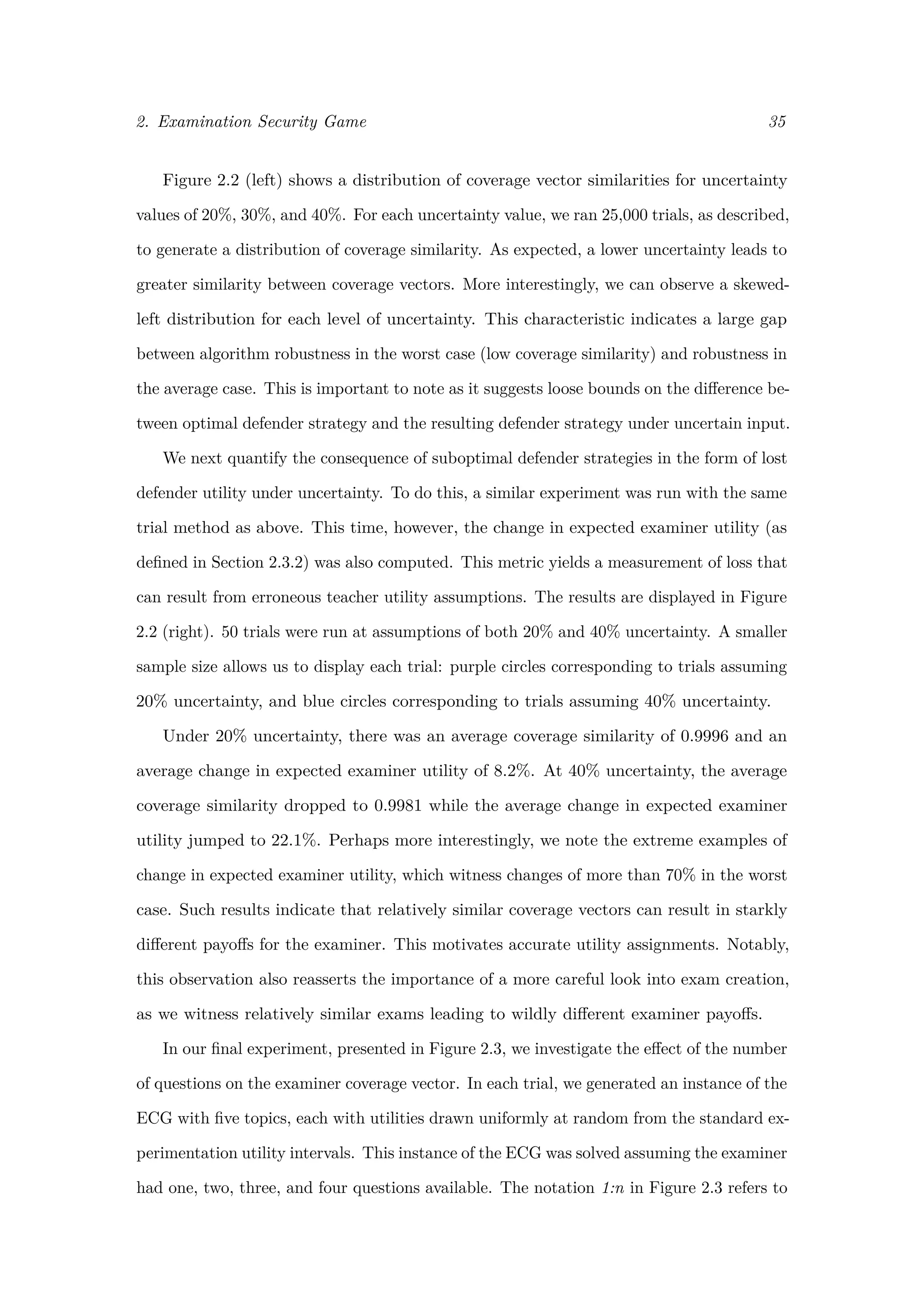
Figure 2.2: Uncertainty and coverage Similarity
between the potential size of error in the input and the change in the suboptimal
coverage vector. We now present this method explicitly.
First, we generate utility values for 5 targets, chosen independently and uniformly
at random from the standard experimentation utility intervals.
Using our implementation of the ERASER algorithm, we find an optimal mixed strategy
for the examiner based on these drawn utilities, assuming that there are 2 available exam
questions (m = 2). We represent this mixed strategy by the coverage vector c, where each
component ci indicates the marginal probability that topic ti is covered on the exam.
Next, for each target t, we draw two values uniformly at random from the interval
[−u, +u]. Denote these values as u1 and u2. Please note that we refer to an assumption
of 20% as an experiment trial with u1, u2 randomly drawn from the interval [−.2, .2].
This notation is inspired by the possibility that original utility values could have an error
of up to 20%. We scale the attacker utility values in the following fashion:
• Uc
A(t) = Uc
A(t) · u1 ∀t ∈ T
• Uu
A(t) = Uu
A(t) · u2 ∀t ∈ T
We once again use our implementation of the ERASER algorithm to find an optimal cover-
age vector c† for the modified inputs. Using cosine similarity, we compare the two coverage
vectors:
Sc(c, c†) =
c · c†
||c|| · ||c†||

41. 2. Examination Security Game 35
Figure 2.2 (left) shows a distribution of coverage vector similarities for uncertainty
values of 20%, 30%, and 40%. For each uncertainty value, we ran 25,000 trials, as described,
to generate a distribution of coverage similarity. As expected, a lower uncertainty leads to
greater similarity between coverage vectors. More interestingly, we can observe a skewed-
left distribution for each level of uncertainty. This characteristic indicates a large gap
between algorithm robustness in the worst case (low coverage similarity) and robustness in
the average case. This is important to note as it suggests loose bounds on the difference be-
tween optimal defender strategy and the resulting defender strategy under uncertain input.
We next quantify the consequence of suboptimal defender strategies in the form of lost
defender utility under uncertainty. To do this, a similar experiment was run with the same
trial method as above. This time, however, the change in expected examiner utility (as
defined in Section 2.3.2) was also computed. This metric yields a measurement of loss that
can result from erroneous teacher utility assumptions. The results are displayed in Figure
2.2 (right). 50 trials were run at assumptions of both 20% and 40% uncertainty. A smaller
sample size allows us to display each trial: purple circles corresponding to trials assuming
20% uncertainty, and blue circles corresponding to trials assuming 40% uncertainty.
Under 20% uncertainty, there was an average coverage similarity of 0.9996 and an
average change in expected examiner utility of 8.2%. At 40% uncertainty, the average
coverage similarity dropped to 0.9981 while the average change in expected examiner
utility jumped to 22.1%. Perhaps more interestingly, we note the extreme examples of
change in expected examiner utility, which witness changes of more than 70% in the worst
case. Such results indicate that relatively similar coverage vectors can result in starkly
different payoffs for the examiner. This motivates accurate utility assignments. Notably,
this observation also reasserts the importance of a more careful look into exam creation,
as we witness relatively similar exams leading to wildly different examiner payoffs.
In our final experiment, presented in Figure 2.3, we investigate the effect of the number
of questions on the examiner coverage vector. In each trial, we generated an instance of the
ECG with five topics, each with utilities drawn uniformly at random from the standard ex-
perimentation utility intervals. This instance of the ECG was solved assuming the examiner
had one, two, three, and four questions available. The notation 1:n in Figure 2.3 refers to

42. 2. Examination Security Game 36
Figure 2.3: Effect of the number of questions on coverage similarity
the cosine similarity between the coverage vector with 1 available question and the coverage
vector with n available questions. A smoothed distribution over 5000 trials is shown.
Reasonably, one may expect a high degree of similarity between all four coverage
vectors. That is, it seems reasonable that an ideal coverage vector when two questions
are available is very similar to the coverage vector when one question is available, just
scaled by a factor of two. Interestingly, this behaviour was not evidenced by the results.
In general, changing the number of questions available prompted a much greater effect
on the coverage vector than modifying the attacker utilities by 40%. This surprising
result indicates a great need to take a closer look at exam creation. Certainly, however,
such counter-intuitive results are difficult to factor in by a human examiner. Indeed, this
motivates further analysis of teaching to the test with Stackelberg Security Games.
2.5 Summary
There is no doubt that examiners face a remarkably difficult challenge in creating
unpredictable exams which tests students across many topics. In this chapter, we
cast this challenge as a Stackelberg Security Game, taking advantage of this powerful
framework to create exam strategies which minimise the effect of teaching to the test.
To do this, we created a model of the interaction between an examiner and a teacher,
and demonstrated that the same assumptions made by SSGs to fit traditional security
settings also hold within this context. We then implemented the ERASER algorithm
[4], which takes advantage of a concise representation of the game to cast it as a MILP.

43. 2. Examination Security Game 37
We provide runtime analysis on a version of the ERASER algorithm implemented with
Mathematica. Finally, we investigated the effect of uncertain assumptions of teacher
utilities and a varying number of questions on the SSE coverage vector.

44. 3Induced Curriculum Problem
Contents
3.1 Introduction . . . . . . . . . . . . . . . . . . . . . . . . . . . . . 38
3.2 Overview . . . . . . . . . . . . . . . . . . . . . . . . . . . . . . . 40
3.3 Introduction to the ICP by Example . . . . . . . . . . . . . . . 41
3.4 Proficiency, Scoring, and Valuation . . . . . . . . . . . . . . . . 44
3.5 Solving ICPs with Linear Valuation Functions . . . . . . . . . 47
3.5.1 Continuous Knapsack Problem . . . . . . . . . . . . . . . . . . . 48
3.5.2 Casting to CKSP . . . . . . . . . . . . . . . . . . . . . . . . . . . 48
3.5.3 Algorithmic Complexity . . . . . . . . . . . . . . . . . . . . . . . 50
3.6 Solving ICPs with 0-1 Valuation Functions . . . . . . . . . . . 51
3.6.1 0-1 Knapsack Problem . . . . . . . . . . . . . . . . . . . . . . . . 52
3.6.2 Casting to 0-1 KSP . . . . . . . . . . . . . . . . . . . . . . . . . 52
3.6.3 Algorithmic Complexity . . . . . . . . . . . . . . . . . . . . . . . 54
3.7 Solving ICPs with Stepped Valuation Functions . . . . . . . . 55
3.7.1 Precedence Constrained Knapsack Problem . . . . . . . . . . . . 56
3.7.2 Casting to PCKSP . . . . . . . . . . . . . . . . . . . . . . . . . . 57
3.7.3 Algorithmic Complexity . . . . . . . . . . . . . . . . . . . . . . . 60
3.8 Prerequisites and Topic Structures . . . . . . . . . . . . . . . . 61
3.8.1 Prerequisites . . . . . . . . . . . . . . . . . . . . . . . . . . . . . 61
3.8.2 Topic Structures . . . . . . . . . . . . . . . . . . . . . . . . . . . 61
3.8.3 Splitting a Topic Structure . . . . . . . . . . . . . . . . . . . . . 63
3.8.4 Solving ICPs with a Connected Topic Structure . . . . . . . . . . 65
3.9 Student Types . . . . . . . . . . . . . . . . . . . . . . . . . . . . 67
3.10 Summary . . . . . . . . . . . . . . . . . . . . . . . . . . . . . . . 69
3.1 Introduction
In this chapter, we present the Induced Curriculum Problem (ICP). The idea behind
the ICP is to create a problem which very closely models the setting in which a teacher
38

45. 3. Induced Curriculum Problem 39
attempts to perfectly teach to the test. We make the assumption that the teacher has
knowledge of the exam, namely what topics will be covered and to what difficulty level
those topics will be assessed. Given this information, the teacher aims to allocate her time
in a fashion which maximises student exam scores. To solve this allocation optimisation
problem, we leverage well-studied variations on the knapsack problem (KSP). By finding
the allocation of class time for a teacher who perfectly teaches to the test, we hope to
gain insight into how curriculum is affected as a result of examination content.
At the heart of the ICP are valuation functions, which map the time spent learning
a topic to an exam score. These valuation functions are a composition of proficiency
functions, which map time spent learning a topic to a proficiency, and scoring functions
which map topic proficiency to an exam score. We interpret a number of realistic forms
of proficiency functions and scoring functions, and provide corresponding algorithms
which find optimal allocations of teaching time in each setting.
We also introduce the notion of topic structures. In short, topic structures rep-
resent prerequisite relationships amongst course topics. We present several tools for
handling complex topic structures within instances of the ICP.
Finally, we introduce multiple student types to the ICP. In a typical classroom setting,
an instructor is charged with preparing many students, all with varying abilities, for
the same exam. Notably, within the context of the ICP, this scenario is handled by
representing distinct student types with a distinct set of proficiency functions. When
multiple student types are present, the notion of an optimal allocation of teaching
time becomes non-trivial, as a strategy that is preferable for one student may leave
another student worse off. With this in mind, we close with a discussion on how to
model realistic notions of classroom social welfare within the ICP.
In Section 3.2, we provide an overview of the components which will influence our
model. In Section 3.3, we provide an example to give insight into the reasoning behind
our model choices. In Section 3.4, we formally present the ICP. Sections 3.5, 3.6,
and 3.7 leverage variations on the KSP to solve instances of the ICP which exhibit
particular features. In Section 3.8, we introduce the notion of prerequisites, and provide
an algorithm which allows us to solve for instances of the ICP which contain prerequisite

46. 3. Induced Curriculum Problem 40
relationships. In Section 3.9, we introduce the typed-ICP, where a teacher must account
for a classroom full of students who have different learning capabilities, and discuss
notions of optimality relevant to the high-stakes testing setting.
3.2 Overview
Before formally defining the the Induced Curriculum Problem, we first give an overview
of several key features of our model in order to provide a degree of intuition. An
instance of the ICP accounts for the following characteristics:
• Fixed amount of teaching time: The teacher has a set amount of class time.
We assume that the amount of teaching time is not sufficient to allow for student
mastery of all topics, so the teacher seeks to find the optimal use of the available
time to maximise student test scores.
• Range of topic difficulty: Each exam question assesses a student on one topic
at a specified difficulty level. A student may have sufficient proficiency in a topic to
answer easier questions on the topic, but is unable to answer more difficult questions.
• Proficiency functions: Each topic has a proficiency function which gives the
relation between time spent being taught a topic and student proficiency in the
topic. Topics exhibit unique learning curves, which introduces a complex trade-off
situation in allocating class time.
• Topic structure: Topics may have prerequisites. That is, before gaining any
proficiency in one topic, a student may need a required level of proficiency in a
different topic or set of topics.
• Student types: Some students may find Topic A easy and Topic B difficult, while
others may find the opposite. Within the ICP, this notion is captured by introducing
student types, each with a distinct set of proficiency functions across the set of
topics.
• Social welfare: The teacher’s classtime allocation applies across all student types.
When multiple student types are present, there is no obvious notion of optimal exam
scores. For instance, one instructor may wish to maximise the sum of all student
scores, while another may wish to maximise the number of students who score above

47. 3. Induced Curriculum Problem 41
a certain threshold. These notions are influenced by measures of achievement in
high-stakes testing.
3.3 Introduction to the ICP by Example
A key aspect of the ICP stems from the fact that the exam can test students on different
proficiency levels within a topic. A student, meanwhile, will gain more advanced proficiency
in a topic if additional time is allocated to teaching that topic, allowing her to answer
more difficult questions. Before providing formal definitions of proficiency functions,
scoring functions, and valuation functions, we begin with an example. Please note that,
throughout this example, we make the simplifying assumption that the teacher has only
one student. In fact, this assumption is made until the introduction of student types in
Section 3.9 in order to simplify notation and increase clarity by separating concepts.
In our example, a teacher is preparing her lone student for a mathematics exam. The
exam will cover two topics:
• t1: Addition
• t2: Subtraction
The ICP model assumes that the teacher has knowledge of what the exam will assess, and
to what degree of difficulty it will be assessed. The motivation behind this assumption
is inspired by the availability of previous exams to teachers. However, while the Exam
Security Game requires that this knowledge is based off of the content from previous exams,
we do not make the same assumption within the context of the ICP. As we will discuss in
detail in Section 3.4, we instead simply assume that the teacher has access to a scoring
function, which provides a score for a given level of student proficiency. Nevertheless, to
illustrate the inspiration behind the ICP model, we will use this case study to provide an
example of how a teacher may formulate a simple scoring function based on previous exams.
Returning to our example, the teacher finds that, historically, both addition and
subtraction have been tested by asking the student to perform the operation on two
positive integers of up to 3 decimal digits in size (with both integers of the same size). We
will refer to these questions as “tier n” for the operation on two n digit numbers (e.g. tier

48. 3. Induced Curriculum Problem 42
Addition Subtraction
Tier 1 Tier 2 Tier 3 Tier 1 Tier 2 Tier 3
2012 1 0 1 1 1 0
2013 1 1 0 1 0 1
2014 0 1 1 1 1 0
2015 1 0 1 1 1 0
2016 1 1 0 1 1 0
Total 4 3 3 5 4 1
Table 3.1: Sample Mathematics Exams from 2012-2016
Addition Subtraction
Tier 1 Tier 2 Tier 3 Tier 1 Tier 2 Tier 3
Cumulative value 4 7 (= 3 + 4) 10 (= 7 + 3) 5 9 10
Table 3.2: Sample scoring relation
2 addition for the addition of two 2-digit numbers). In the past five years, the questions
have been weighted equally and asked with the frequencies shown in Table 3.1.
Using the previous five years exams to form a prediction of this year’s exam, a
teacher can develop a simple scoring relation by accumulating the frequency across
tiers for both addition and subtraction. In the Table 3.2, we show the relation be-
tween a student’s level of proficiency and the number of questions that she would
have been able to answer on the exams of the past five years, in each topic. In our
example, this value will be denoted as a score for the topic.
According to this scoring relation, if the instructor can teach a student up to and
including tier 2 addition as well as tier 1 subtraction, she will receive a score of 7 + 5 = 12.
If instead, she teaches the student tier 1 addition and up to and including tier 2 subtraction,
she will receive an expected payoff of 9 + 4 = 13, a preferred outcome. However, she
only has a fixed amount of teaching time, and knows that she can teach the student
addition and subtraction with the time allocations shown in Figure 3.1.
From the time allocations displayed in Figure 3.1, we can develop a proficiency relation,
which maps each tier to the time required to become sufficiently proficient in the topic
to answer questions on that tier and below, as shown in Table 3.3.
Considering the case where the teacher has six hours of class time, she will max-
imise her score if she allocates all six hours to teaching addition. If she does this,
her student will be sufficiently proficient with addition to perform tier 1 and tier 2

49. 3. Induced Curriculum Problem 43
Figure 3.1: Sample teaching progression
Addition Subtraction
Tier 1 Tier 2 Tier 3 Tier 1 Tier 2 Tier 3
Cumulative time required (hours) 4 6 7 5 8 10
Table 3.3: Sample proficiency relation
addition, resulting in a score of 7 according to the scoring relation. However, if the
teacher only has five hours, she will maximise her expected payoff if she allocates
all five hours to teaching subtraction, which will yield a score of 5. Already, this
example demonstrates a knapsack-like optimisation problem.
A graph representation of the relationships between time and score for each topic,
as shown in Figure 3.2 gives some insight into the tradeoffs faced by the teacher.
While we assume tiered learning in this example, in reality, a student may learn
topics more incrementally. Likewise, an exam may test skills more incrementally. For
instance, with regards to addition, it is reasonable to assume that at a point between
having proficiency sufficient for tier 1 addition and having proficiency sufficient for
tier 2 addition, a student is capable of adding a one-digit and a two-digit number.
Drilling down further, a student may be capable of performing easier tier 2 additions
Figure 3.2: Sample valuation relation

50. 3. Induced Curriculum Problem 44
before solving more difficult tier 2 additions. To handle this, in the following section
we introduce proficiency functions and scoring functions.
3.4 Proficiency, Scoring, and Valuation
Topic proficiency is a measure of capability of a student. It gives a ranking to questions,
according to difficulty, and allows us to decide which topic questions a student can and can-
not successfully answer. Given a topic t, if a student has proficiency αt in topic t, she will
be able to answer a question on topic t if and only if that question requires proficiency ≤ αt.
Formally,
Definition 2. An exam question is a pair (t, αt), where t denotes the topic and αt ∈ [0, 1]
denotes the required level of proficiency in t to provide a correct solution.
Borrowing from the Utility Representation Theorem [34], within a topic, we require
exam questions to satisfy the following relationships, given any questions q1 = (t1, α1), q2 =
(t2, α2), q3 = (t3, α3):
1. Completeness: Either α1 ≤ α2 or α2 ≤ α1. Or both, in which case q1 can be
answered correctly by a student if and only if q2 can be answered correctly.
2. Transitivitiy: If α1 ≤ α2 and α2 ≤ α3, then α1 ≤ α3
For all exam questions within a topic, we assume these relationships are satisfied and
can thus create an ordering of questions (q1, q2, . . . , qk) such that a student being able to
answer question qi implies she is sufficiently proficient in the topic to answer questions
q1, q2, . . . , qi−1 as well [34]. As such, we can assign a student a proficiency α such
that αi ≤ α ≤ αi+1. With this value, we have all the necessary information for
determining which questions a student can and cannot answer.
For simplicity, we require that all proficiencies are rated on the interval [0, 1], where a
proficiency of 0 implies a student can answer no questions on the topic and a proficiency
of 1 implies a student can answer any question on the topic. We formulate the notion
of proficiency as above in order to avoid making any assumptions of exact measures
of student abilities. For instance, it is reasonable to give a ranking to questions
in terms of difficulty, but defining each one on an interval [0, 1] is an unreasonable

51. 3. Induced Curriculum Problem 45
assumption. Instead, proficiency is a ranking, similar to the notion of utility in the
study of economics, which we simply constrain to the interval [0, 1].
The notion of proficiency allows us to formally define scoring functions and profi-
ciency functions. Scoring functions, similarly to the sample scoring relation in Table
3.2, give a mapping from proficiency in a topic to a score. Proficiency functions,
in the spirit of the sample proficiency relation in Table 3.3, give a mapping from
time spent learning a topic to proficiency in that topic.
Definition 3. Given a topic t and a student who has proficiency αt ∈ [0, 1] in t, a scoring
function for t is a monotonic increasing function gt : [0, 1] → R≥0 which gives a score
gt(αt).
Within the greater context of teaching to the test, the scoring functions embody
what an instructor believes will be covered on the exam. While we do not make any
assumptions as to how exactly these functions are defined, we note that a teacher can
define scoring functions based on previous exams, as shown in our example. However, it
is also plausible that a teacher forms scoring functions based on a hunch, newly reviewed
education standards, or some other independent source of information.
We make no assumptions regarding the form of scoring functions, besides their
monotonicity. We do, however, bring particular attention to the importance of step
functions within the context of the ICP. Exams which assess student proficiency based on
a set of questions at fixed proficiency levels are characterized by scoring functions which
are step functions. That is, a student’s score is only increased if her proficiency passes
some threshold. Proficiency functions of this form will be discussed in detail in Section 3.7.
We now introduce proficiency functions.
Definition 4. Given a topic t, a proficiency function for t is a monotonic increasing
function Lt : R≥0 → [0, 1] which gives a mapping from the amount of time (in hours) a
student is taught that topic, denoted at, to the level of proficiency in that topic, denoted
αt, such that the student can answer an exam question (t, α) if and only if αt ≥ α.
In every instance of the ICP, we make the critical assumption that a teacher has a
limited amount of class time which must be optimally allocated. However, depending

52. 3. Induced Curriculum Problem 46
on the classroom context and teacher preferences, allocation of teaching time may be
limited by a degree of granularity. For instance, consider a year 8 algebra class which
has 90 days of 1 hour classroom sessions. An instructor may want to focus on only
one topic each session. Another teacher may break each session into two equal parts
with each potentially covering a different topic. In these scenarios, we must allow for
limited granularity in allocating time, instead of assuming the ability for continuous time
allocation. To account for this, given a minimum allocation granularity of δ hours, we
transform a continuous proficiency function L∗
t to a step proficiency function:
Lt(at) = L∗
t (
at
δ
· δ)
Because of granularity in time allocation, step functions are an important class of
proficiency functions to consider in the context of the ICP. This class of proficiency
functions will also be discussed in detail in Section 3.7.
Now that we have introduced scoring functions and proficiency functions, we can
formally define a valuation function. In words, a valuation function is simply the
composition of a proficiency function and a scoring function that allows for a direct
mapping from time allocated to learning a topic to a score.
Definition 5. Given a topic t, a scoring function for t, denoted gt, and a proficiency
function for t, denoted Lt, a valuation function for t is the function Vt = gt ◦ Lt.
rem. Because scoring functions and proficiency functions are both necessarily monotonic
increasing functions, valuation functions are also monotonic increasing functions.
Finally, we formally present the ICP:
Definition 6. An instance of the ICP is a structure T, GT , LT , Z , where T = {t1, t2, . . . , tn}
is a topic set, GT = {gt1 , gt2 , . . . , gtn } is a set of scoring functions with each gti denoting a
scoring function for ti, LT = {Lt1 , Lt2 , . . . , Ltn } is set of proficiency functions with each
Lti denoting a proficiency function for ti, and Z is the number of hours available for
teaching. A solution to T, GT , LT , Z is written as A = {at1 , at2 , . . . , at3 } which solves
the following optimisation problem:

53. 3. Induced Curriculum Problem 47
Figure 3.3: Formation of linear valuation functions
max
t∈T
gt ◦ Lt(at)
subject to
t∈T
at ≤ Z
and at ≥ 0 ∀t ∈ T
3.5 Solving ICPs with Linear Valuation Functions
The first subset of ICP instances that we will investigate is those which exhibit linear valu-
ation functions. Formally, we will be looking at instances of the ICP, T, GT , LT , Z , such
that for each t ∈ T and the corresponding functions gt ∈ GT , Lt ∈ LT , Vt = gt ◦Lt is a func-
tion of the form:
Vt(at) =
vt · at for at ≤ ct
vt · ct for at > ct
with ct > 0, vt > 0. We will refer to an ICP of this form as an ICP with linear valuation
functions.
While not strictly necessary, perhaps the most important formation of an ICP with
linear valuation functions results from linear proficiency functions and linear scoring
functions, as illustrated in Figure 3.3. A linear proficiency function represents a constant
rate of increase in proficiency as a function of time spent learning a topic, until maximum
proficiency is reached. A linear scoring function captures a scenario where an exam
assesses a student’s abilities uniformly across the proficiency scale. It is important to
note that, while perfectly linear valuation functions are unlikely to occur in real-world
scenarios, they could serve to provide close approximations. Additionally, they offer

54. 3. Induced Curriculum Problem 48
interesting analysis through a casting to the continuous knapsack problem, which will
lead us into an investigation on more interesting instances of the ICP.
3.5.1 Continuous Knapsack Problem
The continuous knapsack problem (CKSP) is a relaxation of the 0-1 knapsack problem
(presented in Section 3.6.1) which allows items to be added to the knapsack in fractional
values. In an instance of the CKSP, we are presented with a set N of n items numbered
from 1 to n. Each item i has a weight wi ∈ Z+ and a value vi ∈ Z+, and we have a
knapsack with capacity C ∈ Z+. The CKSP requires us to maximise the total value of
items within the capacity constraint. Presented as an optimisation problem:
max
n
i=1
vi · xi
subject to
n
i=1
wi · xi ≤ C
and 0 ≤ xi ≤ 1 for i = 1, 2, . . . , n
We denote an instance of CKSP as a structure N, W, V, C , where W = {w1, w2, . . . , wn}, and V =
{v1, v2, . . . , vn}. The solution is the set X = {x1, x2, . . . , xn}. We denote the sum n
i=1 vi ·
xi as k(X).
3.5.2 Casting to CKSP
Given an instance of the ICP with linear valuation functions, denoted as T, GT , LT , Z ,
we produce an instance of the CKSP. Denoting T = {t1, t2, . . . , tn}, we create a set N of n
items where item i has weight wi = cti and value vi = vti ·cti . We set our knapsack capacity
C = Z.
Claim. For instances the ICP T, GT , LT , Z with T = {t1, t2, . . . , tn} and the correspond-
ing functions gti ∈ GT , Lti ∈ LT , Vti = gti ◦ Lti of the form:
Vti (ati ) =
vti · ati for ati ≤ cti
vti · cti for ati > cti
with ct > 0, vt > 0, we denote the solution to the CKSP {1, 2, . . . , n}, {ct1 , ct2 , . . . , ctn }, {vt1 ·
ct1 , vt2 · ct2 , . . . , vtn · ctn }, Z} as X = {x1, x2, . . . , xn}, calculate ati = cti · xi, and claim
that A = {at1 , at2 , . . . , atn } is a solution to the ICP instance T, GT , LT , Z .

55. 3. Induced Curriculum Problem 49
Proof. We first remark that the ICP constraint t∈T at ≤ Z is met. By the capacity
constraint on the CKSP, we know that n
i=1 cti · xi ≤ Z :
Z ≥
n
i=1
cti · xi
=
n
i=1
ati
=
t∈T
at
We also note that each ati ≥ 0, resulting from xi ∈ [0, 1] and cti > 0 with ati = xi · cti .
We demonstrate that A is a maximal solution in a proof by contradiction by assuming
that there is some valid allocation B which yields a more optimal solution to the ICP. We
then show that, if this was the case, there would then exist a more optimal solution to the
corresponding knapsack problem. Formally, we claim that there is some valid allocation
B = {bt1 , bt2 , . . . , btn } such that:
n
i=0
Vti (bti ) >
n
i=0
Vti (ati )
n
i=1
bti ≤ Z
bti ≥ 0 for i = 1, 2, . . . , n
From B, we construct a more optimal solution to the corresponding CSKP, denoted
with Y . We define a mapping from each element bi to element yi ∈ Y :
yi = min{bti /cti , 1}
Note that Vti (bti ) = vti · cti · yi. To see this, we break into two cases: (i) If bti ≥ cti ,
then yi = 1 and Vti (bti ) = vti · cti , as defined by Vti , and we are done, as . (ii) If bti < cti ,
then yi = bti /cti and Vti (bti ) = vti · bti = vti · cti · yi
Now, using our assumption that B yields a more optimal solution to the ICP, we show
that k(Y ) > k(X):

56. 3. Induced Curriculum Problem 50
k(Y ) =
n
i=1
vti · cti · yi
=
n
i=1
Vti (bti ) (as shown above)
>
n
i=1
Vti (ati ) (by assumption)
=
n
i=1
vti · ati (by ati ≤ cti as xi ≤ 1)
=
n
i=1
vti · cti · xi
= k(X)
It remains only to show that Y meets the constraints of the CKSP. First, we claim
that each yi ∈ [0, 1]. This follows from our definition of yi = min{bti /cti , 1}, with cti > 0
by assumption and bti ≥ 0 by the ICP constraints.
Finally, we claim that Y satisfies the capacity constraint of the knapsack problem:
Z ≥
n
i=1
bti (by assumption)
≥
n
i=1
cti · yi
We conclude that Y meets the constraints of the knapsack problem and k(Y ) > k(X).
This contradicts our assumption that X is a solution to the knapsack problem.
3.5.3 Algorithmic Complexity
The CKSP can be solved in polynomial time with a greedy algorithm. In words,
the algorithm orders the items by their ratio of value to weight and fills the knap-
sack in order of decreasing value density until the bag is full [35]. Given n items,
this algorithm requires O(n log n) time to sort the items, and O(n) time to fill the
knapsack using the sorted list. The total runtime is thus O(n log n) time for this
greedy algorithm. In fact, however, the CKSP can be solved in O(n) time by ap-
plying a variation of the Weighted Median Problem [36].
Within the context of the ICP, each topic corresponds to exactly one item in the
CKSP. Casting an instance of the ICP over n topics with linear valuation functions to an

57. 3. Induced Curriculum Problem 51
Figure 3.4: Formation of 0-1 valuation functions
instance of the CKSP requires O(n) time. Furthermore, finding a solution to the ICP
with a solution of the CKSP also requires O(n) time. We conclude that an instance of the
ICP with n topics with linear valuation functions can be optimally solved in O(n) time.
3.6 Solving ICPs with 0-1 Valuation Functions
We now explore the subset of ICP instances where each topic exhibits a 0-1 valuation
function. In these instances of the ICP, a student receives an increase in score, vti , if
and only if the time spent learning topic ti exceeds some threshold a†
ti
> 0, for that
topic. That is, for instances of the ICP T, GT , LT , Z with T = {t1, t2, . . . , tn} and the
corresponding functions gti ∈ GT , Lti ∈ LT , Vti = gti ◦ Lti is of the form:
Vti (ati ) =
vti if ati ≥ a†
ti
0 otherwise
with vti > 0. We will refer to an ICP of this form as an ICP with 0-1 valuation
functions, a name inspired by the 0-1 knapsack problem.
Figure 3.4 summarises several important formations of this class of valuation functions
within the context of an ICP. In particular, we draw attention to the combination of
any general proficiency function and a single step scoring function. Such a scoring
function rewards students if and only if their proficiency is above a defined threshold in
each topic. Common examples of these scoring functions would be factual recollection
exams. For instance, consider a spelling test where a student will be asked to spell
a subset of words from a large bank of possibilities. We also assume that no partial
credit is awarded for any incorrect spellings. In this scenario, we can consider each
word a distinct topic, where a student receives a positive score on a topic if and only if

58. 3. Induced Curriculum Problem 52
they can spell the word correctly. A student either knows the correct spelling or does
not know the correct spelling, which yields a single step scoring function. Within the
context of the ICP, we will use the 0-1 knapsack problem to find an optimal allocation
of teaching time under the assumption of 0-1 valuation functions.
3.6.1 0-1 Knapsack Problem
The 0-1 knapsack problem (KSP) is a well-known combinatorial optimisation problem.
In an instance of the 0-1 KSP, like the CKSP, we are presented with a set N of
n items numbered from 1 to n. Each item i has a weight wi ∈ Z+ and a value
vi ∈ Z+. We have a knapsack with capacity C ∈ Z+, and we must find a subset
S ⊆ N such that i∈S vi is maximised while the total weight i∈S wi ≤ C. Using
a binary variable xi to indicate whether item i is included or not (xi = 1 indicates
item i is included, xi = 0 indicates item i is not included), the knapsack problem
can be presented with an integer programming formulation:
max
n
i=1
vi · xi
subject to
n
i=1
wi · xi ≤ C
and xi ∈ {0, 1} for i = 1, 2, . . . , n
Using the notation introduced above, we denote an instance of 0-1 KSP as a structure
N, W, V, C , where W = {w1, w2, . . . , wn}, and V = {v1, v2, . . . , vn}. The solution is
the set X = {x1, x2, . . . , xn}, and we denote the sum n
i=1 vi · xi as k(X).
3.6.2 Casting to 0-1 KSP
Given an instance of the ICP with 0-1 valuation functions, denoted as T, GT , LT , Z , we
produce an instance of the 0-1 KSP which we can solve using well-studied algorithms.
Using the solution, X, to the 0-1 KSP, we can formulate a solution to the ICP.
Claim. For instances the ICP T, GT , LT , Z with T = {t1, t2, . . . , tn} and the correspond-
ing functions gti ∈ GT , Lti ∈ LT , Vti = gti ◦ Lti of the form:
Vti (ati ) =
vti if ati ≥ a†
ti
0 otherwise

59. 3. Induced Curriculum Problem 53
with vti > 0, a†
ti
> 0, we denote the solution to the 0-1 KSP {1, 2, . . . , n}, {a†
t1
, a†
t2
, . . . , a†
tn
}, {vt1 , vt2 , . . . , vt
as X = {x1, x2, . . . , xn}, calculate ati = xi · a†
ti
, and claim that A = {at1 , at2 , . . . , atn } is
a solution to the ICP instance T, GT , LT , Z .
Proof. We first remark that the ICP constraint t∈T at ≤ Z is met. By the corresponding
knapsack constraint, we know that n
i=1 a†
ti
· xi ≤ Z :
Z ≥
n
i=1
a†
ti
· xi
=
n
i=1
ati
=
t∈T
at
We also note that each ati ≥ 0 as xi ∈ {0, 1} and a†
ti
> 0 with ati = xi · a†
ti
We
demonstrate that A is a maximal solution in a proof by contradiction by claiming that
there is some valid allocation B = {bt1 , bt2 , . . . , btn } such that n
i=0 Vti (bti ) > n
i=0 Vti (ati ).
Using this assumption, we contradict the assumption that X is a solution to the knapsack
problem. To do this, we first define a transformation from each element bti to b∗
ti
by the
function fti :
fti (bti ) =
a†
ti
if bti ≥ a†
ti
0 otherwise
We remark that Vti (bti ) = Vti (fti (bti )) for i = 1, 2, . . . , n. To show this, we break
into two cases: (i) in the case that bti ≥ a†
ti
, it follows that Vti (bti ) = vti = Vti (a†
ti
) =
Vti (fti (bti )); (ii) in the case that bti < a†
ti
, it follows that Vti (bti ) = 0 = Vti (a†
ti
) =
Vti (fti (bti )).
Using B, we construct Y = {y1, y2, . . . , yn} with each yi = b∗
ti
/a†
ti
. We now contradict
the assumption that X is a solution to the 0-1 KSP by proving that Y meets the 0-1
KSP constraints and k(Y ) > k(X). First, we claim that each yi ∈ {0, 1}, which follows
immediately from the fact that b∗
ti
∈ {0, a†
ti
}. Next, we claim that Y satisfies the capacity
constraint which follows directly from our assumption that B is a valid solution to the

60. 3. Induced Curriculum Problem 54
ICP:
Z ≥
n
i=1
bti (by assumption)
≥
n
i=1
b∗
ti
(by definition)
=
n
i=1
a†
ti
· yi
Finally, we show that k(Y ) > k(X):
k(Y ) =
n
i=1
vti · yi
=
n
i=1
vti · (b∗
ti
/a†
ti
)
=
n
i=0
Vti (b∗
ti
)
=
n
i=0
Vti (fti (bti ))
=
n
i=0
Vti (bti )
>
n
i=0
Vti (ati ) by assumption
=
n
i=1
vti · xi (by xi ∈ {0, 1})
= k(X)
Thus, Y meets the constraints of the knapsack problem and k(Y ) > k(X). This
contradicts our assumption that X is a solution to the knapsack problem.
3.6.3 Algorithmic Complexity
The 0-1 KSP is a well-known NP-hard problem. While fully-polynomial approximation
schemes do exist [35], their analysis focuses on the closeness to optimality with respect to
total knapsack value. The ICP, however, has been designed with the intention of finding
an optimal allocation of teaching time, thereby providing a means to measure the effect
of high-stakes testing on curriculum deformation. As a result, we will focus on exact
algorithms. Fortunately, pseudopolynomial algorithms have been developed for finding
exact solutions. Given an upper bound on the value of the optimum solution, denoted
B, a dynamic programming algorithm can solve the 0-1 KSP in O(nB) time [37].

61. 3. Induced Curriculum Problem 55
Figure 3.5: Formation of stepped valuation functions with granular time allocation
Casting an instance of the ICP over n topics with 0-1 valuation functions to an instance
of the 0-1 KSP requires O(n) time. Furthermore, transforming a solution to the 0-1 KSP to
a solution of the ICP also takes O(n) time, as both operations involve only multiplication
or division of two integers for each topic. Thus, the total runtime for finding a solution to
the ICP takes O(nB) time, where B is an upper bound on the optimal solution of the ICP.
3.7 Solving ICPs with Stepped Valuation Functions
The next subset of ICP instances that we will investigate is those where the valuation func-
tion for each topic is a step function. That is, for instances of the ICP T, GT , LT , Z such
that for each t ∈ T and the corresponding functions gt ∈ GT , Lt ∈ LT , Vt = gt ◦ Lt can be
written in the form:
Vt(at) =
k
j=0
hBj,bj
(at)
with k ≥ 0 and each hBj,bj
: R → R of the form:
hBj,bj
(a) =
bj if a ≥ Bj
0 otherwise
with Bj > 0, bj > 0.
We will refer to an ICP of this form as an ICP with stepped valuation functions.
Figures 3.5 and 3.6 illustrate important combinations of proficiency functions and scor-
ing functions which result in stepped valuation functions. In particular, Figure 3.5 shows
the case where a teacher has a limited granularity of the allocation on teaching time. Recall
from Section 3.4 that this is represented as a proficiency function that is a step function.

62. 3. Induced Curriculum Problem 56
Figure 3.6: Formation of stepped valuation functions with stepped scoring
Another important scenario to consider is when the scoring functions are step functions,
as shown in Figure 3.6. This is the case when an exam assesses students at one or more
fixed levels of proficiency. Consider, for instance, if an exam board releases tests with
questions that assess the same level of proficiency, but reword the question or change values
to make sure students cannot memorise answers from previous exams. In this case, step
functions capture the relationship between student proficiency and exam score very well.
Before we present an algorithm for finding solutions to instances of the ICP with
stepped valuation functions, we introduce the precedence constrained knapsack problem.
3.7.1 Precedence Constrained Knapsack Problem
The precedence constrained knapsack problem (PCKSP), also known as the partially
ordered knapsack problem, is a generalised version of the 0-1 knapsack problem which takes
into account precedence requirements between items. That is, given a set of items N, a
precedence relation exists between two items (i, j) ∈ N × N if and only if the item i can
be placed in the knapsack only on the condition that item j is also placed in the knapsack
[38]. We denote the set of these precedence relations as R, and represent the PCKSP as
a graph G = (N, R). As with the 0-1 KSP, each item has a value vi and a weight wi,
with the value xi ∈ {0, 1} indicating whether item i is included in the knapsack (with
xi = 1 indicating item i is in the knapsack). We must fill the knapsack to maximise total
value while meeting precedence constraints and a total capacity constraint C. Formally,

63. 3. Induced Curriculum Problem 57
Time Allocation B0 = 0 B1 B2 . . . Bk
Score b0 = 0 b1 b1 + b2 . . . k
i=1 bk
Table 3.4: Table representation of stepped valuation functions
the following presents the PCKSP, formulated as an integer programming problem:
max
i∈N
vi · xi
subject to
n
i=1
wi · xi ≤ C
and xi ≤ xj for all (i, j) ∈ R
and xi ∈ {0, 1} for all i ∈ N
Using the presented notation, we denote an instance of the PCKSP as a structure
N, W, V, C, R , where W = {w1, w2, . . . , wn}, and V = {v1, v2, . . . , vn}. The solution
is the set X = xi for i ∈ N with k(X) denoting the sum i∈N vi · xi.
3.7.2 Casting to PCKSP
Because of the special structure of step functions, we are able to create a more intuitive
table representation of these functions. Using the previously introduced notation, denote
B = {hB1,b1 , hB2,b2 , . . . , hBk,bk
} as the re-indexed list of functions which are sorted in
ascending order according to the values Bj. Without loss of generalisation, we assume
that all Bj are unique. If this was not the case, and there was a pair Bx, By such
that Bx = By, we could simply rewrite the step function
Vt(at) =
k
j=0
hBj,bj
(at)
replacing hBx,bx and hBy,bx with hBz,bz , with Bz = Bx(= By) and bz = bx + by.
The table representation is shown in Table 3.4.
Fact 1. We note that for any topic time allocation at with Vt(at) = st, there exists some
allocation Bi ≤ at such that Vt(Bi) = at. As a result, any optimal time allocation can be
achieved by only using the values in the table. This characteristic is critical to solving
instances of the ICP with stepped valuation functions.

64. 3. Induced Curriculum Problem 58
Index (i) 0 1 2 . . . k
Marginal Time Allocation (wi) B0 =0 B1 B2 − B1 . . . Bk − Bk−1
Marginal Score Increase (vi) b0 = 0 b1 b2 . . . bk
Table 3.5: Marginal table representation of stepped valuation functions
Figure 3.7: Graph representation of stepped valuation function
We also define a table where each entry corresponds to the marginal time allocation and
marginal score increase of a step, as shown in Table 3.5. To simplify notation, on a given
step index i, we will refer to the marginal time allocation as wi, and the marginal score in-
crease as vi.
From the marginal table representation in Table 3.5, we produce a graph repre-
sentation G = (N, R). N is the set of vertices {1, . . . , k}. R is the set of edges
which comprises all pairs (i, j) for j = 1, 2, . . . , k and i = j − 1. Figure 3.7 shows
the graph representation of a stepped valuation function.
Given an instance of the ICP with stepped valuation functions, denoted as T, GT , LT , Z ,
we produce an instance of the PCKSP. Denoting T = {t1, t2, . . . , tn}, we first form a
graph representation Gi of each topic ti. For graph Gi, let Ni denote the corresponding
set of vertices, and Ri denote the corresponding set of edges. Let
N =
n
i=1
Ni
R =
n
i=1
Ri
We use the notation vi,j to denote the marginal score increase of the j-th item of set Ni,
and equivalently the value of the j-th vertex of set Ni. Let V denote the set of all values
vi,j. Similarly, we denote wi,j as the marginal time allocation of the j-th item of set Ni, and
equivalently the weight of the j-th vertex of the set Ni. Let W denote the set of all values
wi,j.

65. 3. Induced Curriculum Problem 59
V =
i∈{1,...n} j∈Ni
vi,j
W =
i∈{1,...n} j∈Ni
wi,j
Claim. For instances the ICP T, GT , LT , Z with stepped valuation functions for each
t ∈ T, we form a PCKSP N, W, V, Z, R . We denote the solution as X, with xi,j
indicating if the j-th item of the set Ni is in the knapsack. Let
ati =
j∈Ni
xi,j · wi,j
We claim that A = {at1 , at2 , . . . , atn } is a solution to the ICP.
Proof. We first remark that the ICP constraint t∈T at ≤ Z is met as a consequence of
the PCKSP capacity constraint:
Z ≥
n
i=1 j∈Ni
wi,j · xi,j
=
n
i=1
ati
=
t∈T
at
Additionally, we see that ati ≥ 0 as xi,j ∈ {0, 1}, wi,j ≥ 0 with ati = j∈Ni
xi,j · wi,j.
To show that the ICP is optimally solved, we again use a proof by contradiction. We
claim that there exists some allocation D = {dt1 , dt2 , . . . , dtn } such that:
n
i=0
Vti (dti ) >
n
i=0
Vti (ati )
n
i=1
dti ≤ Z
dti ≥ 0 for i = 1, 2, . . . , n
Without loss of generality, we claim that each dti can be written as the sum:
dti =
j∈Ni
wi,j · yi,j
for yi,j ∈ {0, 1} and yi,j ≤ yi,j−1. This follows from Fact 1.

66. 3. Induced Curriculum Problem 60
We denote the set of yi,j as Y , and use the assumed existence of Y to contradict that
X is a solution to the PCKSP.
We have already remarked that Y meets the precedence constraints and that each
yi,j ∈ {0, 1}, both following from Fact 1. Next, we claim that Y satisfies the capacity
constraint of the PCKSP. This follows from our assumption that D meets the capacity
constraint of the ICP:
Z ≥
n
i=1
dti (by assumption)
=
n
i=1 j∈Ni
wi,j · yi,j (by definition)
Finally, we see that k(Y ) > k(X) :
k(Y ) =
n
i=1 j∈Ni
vi,j · yi,j
=
n
i=1
Vti (dti )
>
n
i=1
Vti (ati ) (by assumption)
=
n
i=1 j∈N
vi,j · xi,j
= k(X)
Thus, Y meets the constraints of the PCKSP and k(Y ) > k(X). This contradicts our
assumption that X is a solution to the PCKSP.
3.7.3 Algorithmic Complexity
As demonstrated by Johnson and Niemi, the PCKSP is a strongly NP-complete problem
[39]. As such, current algorithms to solve instances of the PCKSP rely on enumeration
methods, such as branch-and-bound [40]. However, pseduopolynomial time algorithms
exist for solving the PCKSP in the case of prerequisite structures which are trees.
This is, in fact, the case in our formulation of the PCKSP if we simply add a dummy
vertex (of value and weight 0) which is connected to the first vertex in each set Ni for
i ∈ {1, 2, . . . , n}. While the tree-version of the PCKSP is still NP-complete [39], dynamic
programming solutions offer improvements on enumeration methods. We do however,

67. 3. Induced Curriculum Problem 61
make a warning regarding the size of the PCKSP which is dependent on the number
of steps in each valuation function, rather than just the number of topics.
3.8 Prerequisites and Topic Structures
3.8.1 Prerequisites
In our analysis from Section 3.5 through Section 3.7, we made the assumption that topics
were entirely independent of one another. That is, we assumed that proficiency in one
topic was never a requirement to acquiring proficiency in another topic. In this section, we
define prerequisites within the context of the ICP, and formally introduce topic structures.
Definition 7. A proficiency prerequisite to learning topic t0 is a pair (t, α), where
α ∈ [0, 1] is the proficiency in topic t required before acquiring any proficiency in topic t0.
Definition 8. A prerequisite proficiency function for topic t0, denoted as Rt0 , maps
each topic t with t = t0 to the proficiency required in t before acquiring proficiency in t0.
Denoting αt0,t as the proficiency in t necessary before acquiring any proficiency in t0, we
define Rt0 (t) = αt0,t.
Definition 9. A topic t is a prerequisite to topic t0 if Rt0 (t) > 0. If having proficiency
in topic t0 αt0 > 0 implies that any question (t, αt) can be succesfully answered, we refer
to t as a full prerequisite of t0. Otherwise, we refer to t as a partial prerequisite of t0.
Please note that this slightly verbose notion of a full prerequisite is a result of
our definition of proficiency, which corresponds to a ranking of questions according to
difficulty. In words, if t is a full prerequisite of t0, it simply implies that a student
must have full mastery of t before gaining any proficiency in t0.
3.8.2 Topic Structures
We now present the notion of topic structures, which give a representation of any prerequi-
site relationships amongst course topics.
Definition 10. Given a set of topics T = {t1, t2, . . . , tn}, a topic structure of T is the
set {R1, R2, . . . , Rn}, where Ri is the set of prerequisites of ti ∈ T.

68. 3. Induced Curriculum Problem 62
Figure 3.8: Separate, stacked, and tree topic structures
To make the discussion of topic structures more intuitive, we also define a graph repre-
sentation of a topic structure.
Definition 11. Given a set of topics T = {t1, t2, . . . , tn} and its topic structure {R1, R2, . . . Rn},
a graph representation of a topic structure is a directed graph G = (V, E) such that
V = T and an edge (ti, tj, αti,tj ) ∈ E if and only if tj is a prerequisite of ti. If tj is
a full-prerequisite of ti, we define αti,tj = 1. Otherwise, for an edge (ti, tj, αti,tj ) ∈ E,
αi,j = Rti (tj).
In Figure 3.8, we present a visual representation of disconnected, non-unit connected,
and unit connected topic structures. Below, we provide a description for each.
Disconnected Topic Structure
A disconnected topic structure assumes that all topics are independent of each other. In a
disconnected topic structure, teaching material for one topic will not have any influence on
a student’s proficiency in a distinct topic. This topic structure was assumed in our previous
analysis.
An example of a disconnected topic structure is a geography course where students stu-
dents are asked to be proficient in naming the countries of Europe and Asia. In this scenario,
the ability to label the countries of Europe is independent of the ability to label the coun-
tries of Asia.
Definition 12. A set of topics T has a disconnected topic structure if and only if each
element in its topic structure is the empty set. Equivalently, T has a disconnected topic
structure if and only if its graph representation (T, ∅).

69. 3. Induced Curriculum Problem 63
Connected Topic Structure
To be clear, in a disconnected topic structure, each topic has an inner-topic ranking, rep-
resented by the notion of proficiency. A connected topic structure accounts for prerequisites
across separate topics.
Definition 13. A set of topics T has a connected topic structure if and only if it does
not have a disconnected topic structure. Equivalently, T has a connected topic structure if
and only if its graph representation (T, E) with E = ∅.
We will now introduce a special form of connected topic structures- a unit connected
topic structure:
Definition 14. A set of topics T has a unit connected topic structure if every prerequisite
over T is a full prerequisite. That is, for any ti, tj ∈ T , ti is a prerequisite of tj if and
only if ti is a full prerequisite of tj. A connected topic structure that is not a unit topic
structure is referred to as a non-unit connected topic structure.
We take advantage of this special structure to solve instances of the ICP with unit
connected topic structures with a casting to the PCKSP. Making the assumption that all
prerequisites are full prerequisites allows us to place prerequisite constraints which are
analogous to the precedence constraints in the PCKSP. In order to use the same casting to
solve instances of the ICP with non-unit connected topic structures, we present a method
for transforming non-unit connected topic structures into unit connected topic structures.
3.8.3 Splitting a Topic Structure
The transformation from a non-unit connected topic structure to a unit connected topic
structure is handled by splitting topics which are partial prerequisites such that the
resulting topics have full prerequisites relationships. Figure 3.9 provides intuition on this
process. Here, we present it formally as the SPLIT_STRUCTURE algorithm:

70. 3. Induced Curriculum Problem 64
SPLIT_STRUCTURE Algorithm
G = (T, E), a graphical representation of non-unit connected topic structure T =
{t1, . . . , tn}
A graphical representation of an equivalent unit connected topic structure of T
1. Find edge (ti, tj, αti,tj ) such that αti,tj ≤ αta,tb
for all edges (ta, tb, αta,tb
) ∈ E
2. If αti,tj < 1:
(a) (tj1, tj2) ← SPLIT(tj, Rti (tj))
(b) T ← T ∪ {tj1, tj2}
(c) E ← E ∪ {(tj2, tj1, 1)} ∪ {(ti, tj1, 1)}
(d) For each t such that (t, tj, αt,tj ) ∈ E:
i. αt,tj2 ←
αt,tj −αti,tj
1−αti,tj
OR 1 if (t, tj2) is now a full prerequisite relationship
ii. E ← E ∪ {(t, tj2, αt,tj2 )}
iii. E ← E {(t, tj, αt,tj )}
(e) For each t such that (tj, t, αtj,t) ∈ E:
i. E ← E ∪ {(tj1, t, αtj,t)}
ii. E ← E {(tj, t, αtj,t)}
(f) T ← T {tj}
(g) E ← E {(ti, tj, αti,tj )}
(h) Go to Step 1
The aforementioned SPLIT algorithm takes in a target t and a proficiency level
α0 ∈ (0, 1), and returns two targets t1 and t2, where t1 accounts for proficiency from
0 to α0, of the original target t, and t2 accounts for proficiency from α0 to 1. As
a result, the partitioned topics each have their own proficiency functions and scor-
ing functions, denoted by Lt1 and gt1 for i = {1, 2}. Below, we formally generate
the proficiency functions in the natural ways for t1 and t2. We denote a0 ∈ R≥0
as the smallest amount of time such that Lt(a0) ≥ α0:
Lt1 (a) =
1
α0
Lt (a) if a < a0
1 otherwise
Lt2 (a) =
1
1−α0
Lt (a − a0) if a > a0
0 otherwise
We also generate the scoring functions, gt1 , gt2 from the scoring function for t, denoted

71. 3. Induced Curriculum Problem 65
Figure 3.9: Splitting a topic structure
gt:
gt1 (α) = gt (α0 · α)
gt2 (α) = gt α0 +
1
1 − α0
· α − gt(α0)
Figure 3.9 shows an example of splitting a non-unit connected topic structure into
a unit connected topic structure. We note that a non-unit connected topic struc-
ture which originally has n targets and k partial prerequisite relationships will re-
sult in a split topic structure of at most n + k topics.
3.8.4 Solving ICPs with a Connected Topic Structure
In Section 3.7, we showed how to solve an instance of the ICP with stepped valuation
functions and a disconnected topic structure. Keeping in mind that this form of valuation
function plays a particularly important role within the broader context of the ICP, in
this section, we will show how to solve instances of the ICP with stepped valuation
functions and a connected topic structure. To do so, we will make a slight modification
to our casting to the PCKSP, as presented in Section 3.7.2. In short, the algorithm
is performed in three steps: (i) split the topic structure, if necessary, to create a unit
connected topic structure; (ii) cast the ICP to an instance of PCKSP to find the optimal
allocation of teaching time over the split topic structure; (iii) transform the solution
over the split topic structure to a time allocation over the original topic structure. The
algorithm for step (i) has been detailed in the previous section. Here, we present
the casting to PCKSP, which is overviewed in Figure 3.10.
We are provided an instance of the ICP with stepped valuation functions, denoted as
T, GT , LT , Z . We also assume that the topic structure of T, denoted as {R1, R2, . . . , Rn},
is unit connected. As described in Section 3.7, the stepped valuation function of each
topic can be represented as a graph Gi = (Ni, ri), with Ni = {1, 2, . . . , ki} and ri denoting
the set of edges which comprises all pairs (i, j) with j = 1, 2, . . . , ki and i = j −1. Let Ni,j
denote the j-th item of the set Ni. In words, for each pair of topics ti, tj such that tj is a

72. 3. Induced Curriculum Problem 66
Figure 3.10: Generating PCKSP from stepped valuation functions over unit connected topic
structures
prerequisite to ti, we will create an edge from the 1st vertex of the set Ni to the kj-th vertex
of the set Nj. We will then take the union of the sets of edges ri and the set of edges from
prerequisite relationships to create the set of all precedence relationships in an a PCKSP.
More formally, let
N =
n
i=1
Ni
r =
n
i=1
ri
R =
n
i=1
Ri
P =
(ti,tj)∈R
(Ni,1, Nj,kj
)
Let R = P ∪ r. We use the notation vi,j, as done in Section 3.7, to denote the value of
the j-th vertex of graph Gi. Let V denote the set of all values vi,j across all Gi. We denote
wi,j as the weight of the j-th vertex of the set Ni. Let W denote the set of all values wi,j.
V =
i∈{1,...n} j∈Ni
vi,j
W =
i∈{1,...n} j∈Ni
wi,j

73. 3. Induced Curriculum Problem 67
Let X denote the solution to the PCKSP N, W, V, Z, R , with xi,jindicating if the j-th
item of the set Ni is in the knapsack.
All that remains is to cast our solution to the PCKSP back into a solution for the ICP.
Letting
ati =
j∈Ni
xi,j · wi,j
it follows that A = {at1 , at2 , . . . , atn } is a solution to the ICP.
3.9 Student Types
Until now, we have considered instances of the ICP with a single student. These instances
can be represented with a single set of proficiency functions LT . In real-world scenarios,
teachers are often faced with a classroom full of students with different capabilities. Each
student may require a different amount of time allocated to a topic to reach a certain
proficiency level. In our model, different student types can be represented with distinct
proficiency functions. Given a topic set T and a set of students Q = {q1, q2, . . . , qk},
we denote the set of proficiency functions over T for student qi as LT,i.
We also introduce the notion of an objective function F. Previously, we assumed an ob-
jective:
max
t∈T
gt ◦ Lt(at)
With the presence of multiple student types, however, we must account for different
notions of optimality. With this, we present the typed-ICP.
Definition 15. An instance of the typed-ICP is a structure T, GT , QT , Z, F . T =
{t1, t2, . . . , tn} is a topic set. Z is the number of hours available for teaching. GT =
{gt1 , gt2 , . . . , gtn } is a set of scoring functions with each gti denoting a scoring function for ti.
QT = {LT,1, LT,2, . . . , LT,k} is a set where each element ,LT,j = {Lt1,qj , Lt2,qj , . . . , Ltn,qj },
is a set of proficiency functions with each Lti,qj denoting a proficiency function for topic
ti for student type qj. F : Rn → R is an objective function which the ICP aims to
maximise. A solution to T, GT , LT , Z, F is written as A = {at1 , at2 , . . . , atn } which
solves the following optimisation problem:

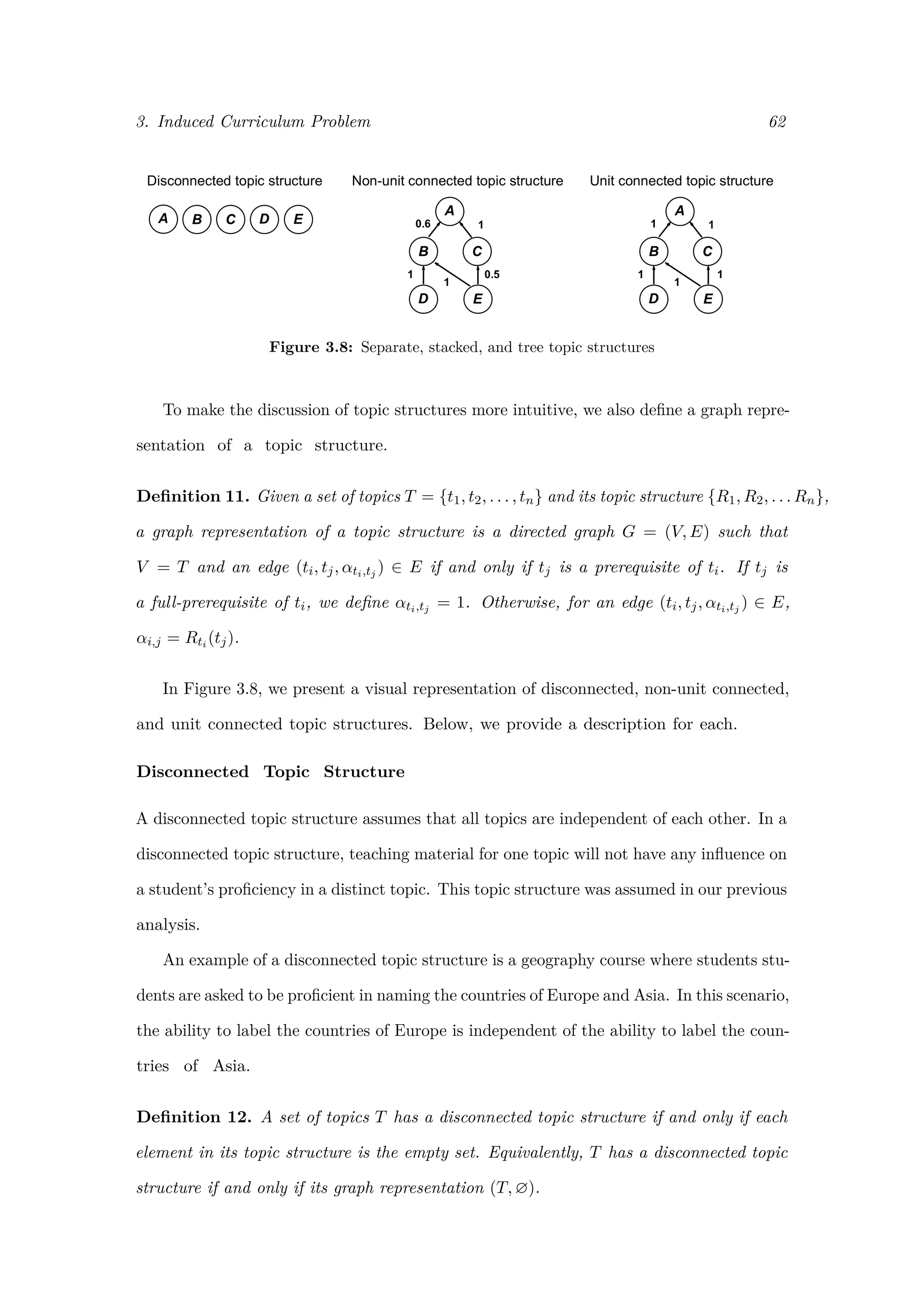
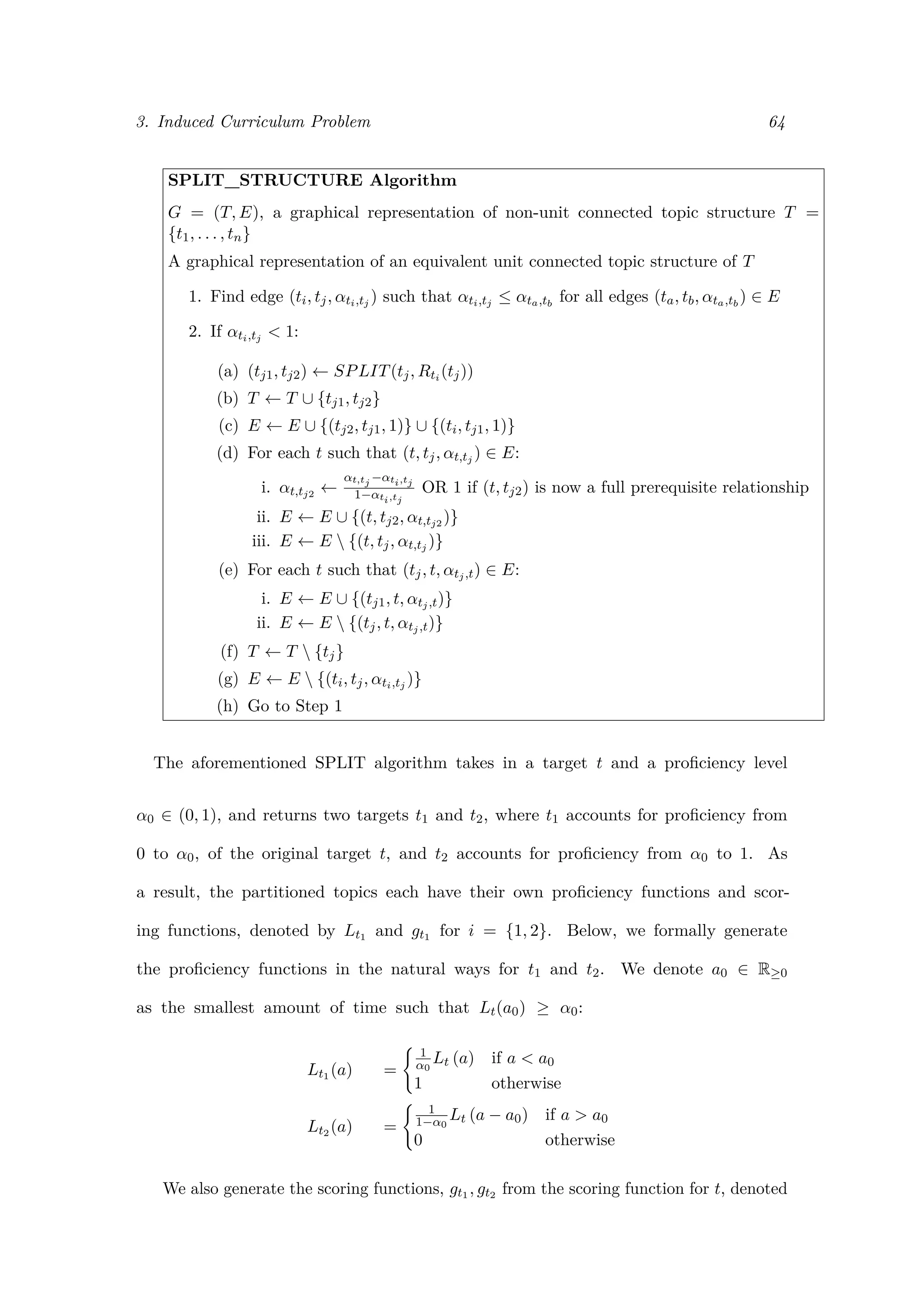
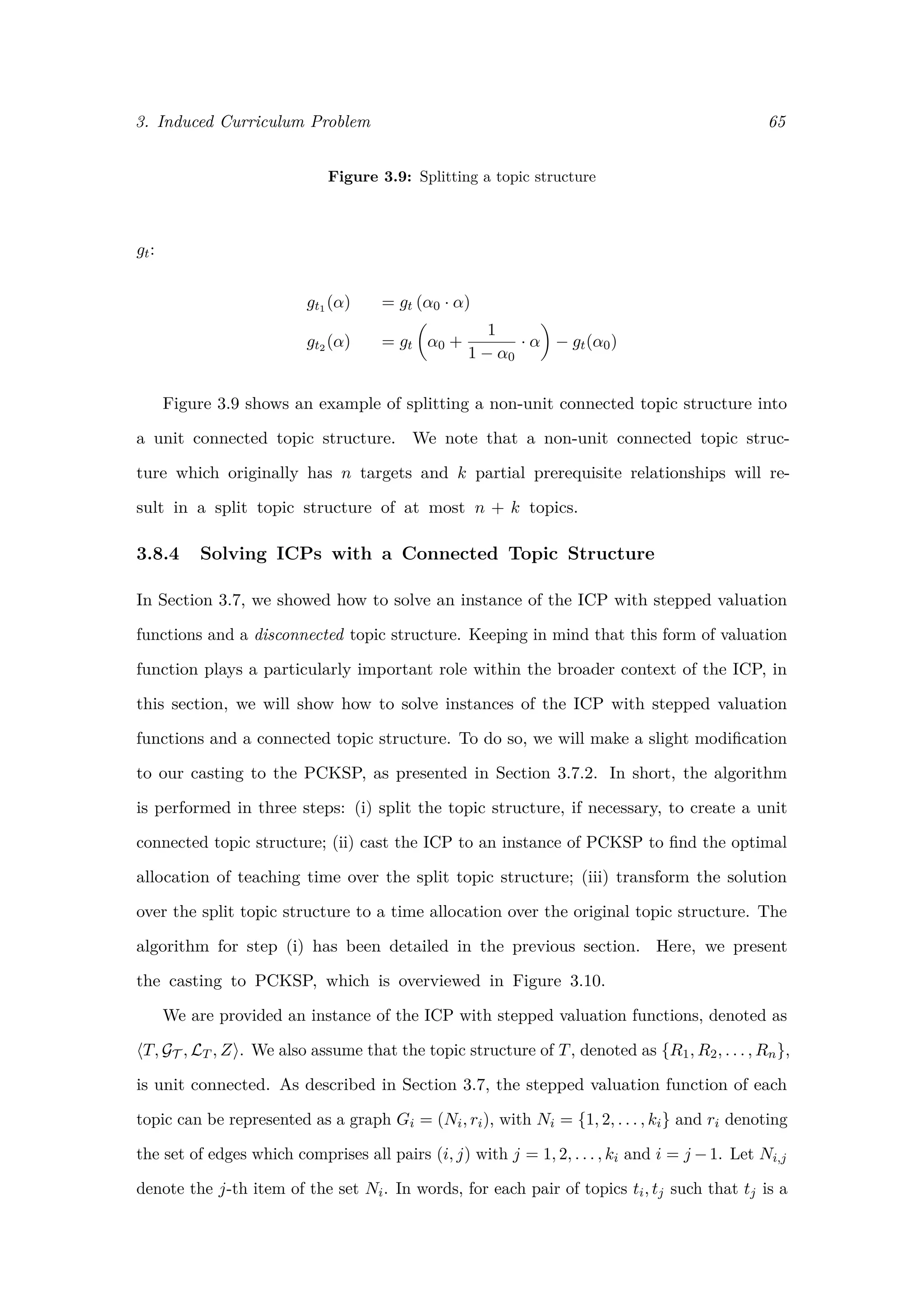
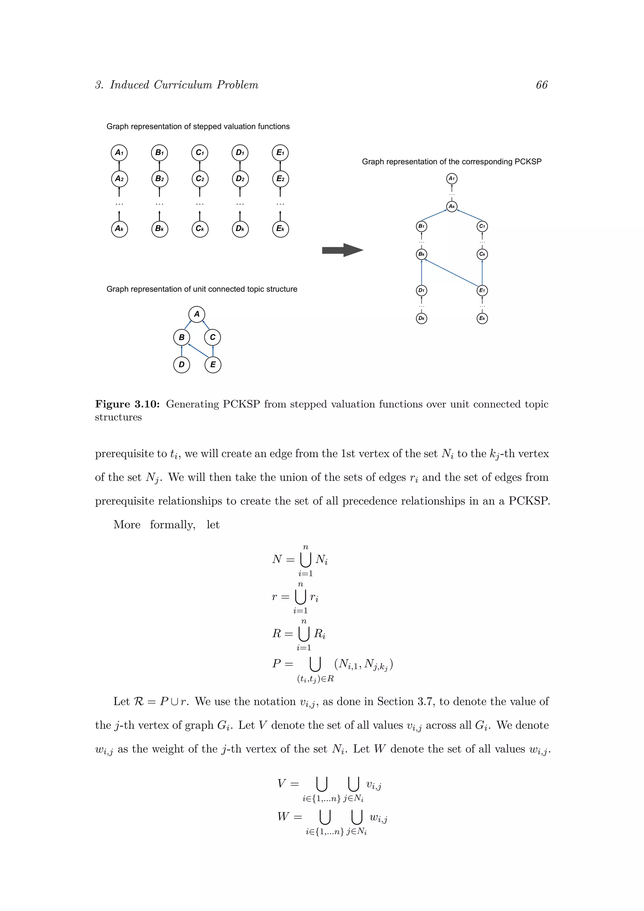
74. 3. Induced Curriculum Problem 68
max F(A)
subject to
t∈T
at ≤ Z
and at ≥ 0 ∀t ∈ T
We first consider an objective function of the following form:
F(A) =
n
i=1
k
j=1
gti ◦ Lti,qj (ati )
In words, a solution to a typed-ICP with this objective function maximises the sum of
test scores across all students. To solve instances of this form, we can create a global valu-
ation function which simply sums over the valuation functions of all students. We denote
Vti (ati ) =
k
j=1
gti ◦ Lti,qj (ati )
It follows that
F(A) =
n
i=1
Vti (ati )
This provides a direct mapping to the optimisation problem of the untyped ICP,
allowing us to use the analysis from Section 3.5 through Section 3.8 to find a optimal
allocations of teaching time assuming this objective function.
More interestingly, consider an objective function which aims to maximise the total
number of students who score above a certain threshold. This idea of optimality is moti-
vated by the importance of the portion of students with C-A* GCSE marks in UK secondary
schools. Brian Lightman, President of the Association of School and College Leaders, ex-
plains:
The focus of GCSEs has been very heavily on the C-D border line, and not,
for example, on students underachieving by getting a grade A, but who could
hopefully get an A*, or on those getting a B, but who could be helped to get
an A [3].
While we do not provide analysis regarding this form of objective function here, it is
nonetheless interesting to note due to its relevance within greater context. Formally, we can
represent the objective function as:

75. 3. Induced Curriculum Problem 69
F(A) =
k
j=1
hθ
n
i=1
gti ◦ Lti,qj (ati )
where
hθ(x) =
1 if x ≥ θ
0 otherwise
3.10 Summary
Teaching to the test in the form of reallocating class time to focus on tested topics is
a well-documented phenomenon, largely attributed to high-stakes testing environments.
Yet, evidence of the precise effect on curricula remain largely anecdotal. We present
the ICP in an effort to quantify the consequences of teaching to the test. To solve
this optimisation problem, we drew natural parallels to generalisations of the knapsack
problem. In an effort to make the model realistic, we explored a range of influencing
factors. We present a summary of these factors below.
• Exam Coverage: To model the general relationship between exams and proficiency,
we introduced scoring functions. While we do not require that scoring functions
are based on previous exams, we suggest this is a reasonable method of formulating
these functions. We brought particular focus to stepped scoring functions, which
result from exams which reward students for achieving benchmarks within each
topic.
• Learning Curves: To account for different learning curves of different topics, we
introduced proficiency functions. Also of note, to account for limited granularity in
allocating teaching time, we used stepped proficiency functions.
• Topic Structure: We presented connected topic structures which exhibited
prerequisite dependencies between topics. Through a casting to the PCKSP, we
were able to solve for instances of the ICP with unit connected topic structures.
Furthermore, we presented the SPLIT_STRUCTURE algorithm which allowed us to
transform non-unit connected topic structures into unit connected topic structures,
allowing us to again leverage the PCKSP to find solutions to the ICP.

76. 3. Induced Curriculum Problem 70
• Student Types: We formulated the typed-ICP to account for different student
types. This modified optimisation problem allows for general objective functions
which can represent different motivations of teachers.

77. 4Further Works
Examination Security Game
There is a significant line of research on Stackelberg Security Games which can be applied
to the ESG. Quantal Response models have been applied to account for boundedly
rational attackers [41]. Within the context of ESGs, teachers may not only be boundedly
rational, but also feel some moral incentive to cover all possible topics. Tendency
driven suboptimal behaviour within SSGs has been previously explored [42], and would
provide interesting insights in our security model examinations.
Furthermore, recent studies on SSGs have presented methods for optimising security
schedules based on deployment data. In particular, processes have been applied in
generating optimal defender strategies taking into account uncertainties in execution and
input [12, 42, 43]. Given the availability of data regarding standardised assessments, we
believe there is a great opportunity to apply methods of machine learning to the ESG.
Finally, the ESG made a number of assumptions regarding test format, some of which
were addressed in a different context within the ICP. Due to already established methods
for taking into account attacker types with Bayesian SSG, we believe this would be a
beneficial area of future work. Furthermore, methods should be developed to take into
account varying question difficulties within the same topic and complex topic structures.
71

78. 4. Further Works 72
Induced Curriculum Problem
We presented solutions to select subsets of the ICP which boasted valuation functions with
special characteristics. A remaining challenge is to develop algorithms to solve the ICP as-
suming general valuation functions.
Additionally, we introduced the notion of student types, but there remains considerable
research left to be done concerning the ICP under different assumptions of optimality.
Perhaps most pressingly, it would be interesting to see an algorithm which solved the typed-
ICP where a teacher aims to maximise the total number of students who score above a
threshold.
We believe it would be beneficial to perform studies on the comparison of ICP solutions
to real-world instances of teaching to the test. If the model shows promise, it would be
interesting to use it in measuring the effect of teaching to the test on different student types
(e.g. is the education of low and high end students compromised due to teaching to the test).
Finally, in order to make full use of the ICP, we recommend the development of a
related game. In the induced curriculum game, examiners would attempt to create a test
which best aligned teacher curricula with the state standards intentions. If successful, the
results of these studies could be considered in generating state standardised exams.

79. Appendices
73

80. AJavaScript Implementation of ERASER Algorithm
1 var _ = require ( ’ lodash ’ ) ;
var d3 = require ( ’ d3 ’ ) ;
3 var f s = require ( ’ f s ’ ) ;
var s o l v e r = require ( ’ javascript −lp−s o l v e r ’ ) ;
5
7 exports . ssgSolver = function ( u t i l i t i e s ) {
var m = 1;
9 var n = u t i l i t i e s . length ;
var z = getZValue ( u t i l i t i e s , m, n) ;
11 var v a r i a b l e s = getVariables (n) ;
13 var o b j e c t i v e = [ "max: d" ] ;
var c o n s t r a i n t s = getConstraintStringArray ( u t i l i t i e s , m, n , z ,
v a r i a b l e s ) ;
15 var integerDomainRestrictions = getDomainArray ( [ ] , n) ;
var stackelbergModel = _. concat ( objective , constraints ,
integerDomainRestrictions ) ;
17
var formattedModel = s o l v e r . ReformatLP ( stackelbergModel ) ;
19 var s o l u t i o n = s o l v e r . Solve ( formattedModel ) ;
21 return s o l u t i o n ;
23 function getAttackConstraint ( u t i l i t i e s , m, n , z ) {
var constraint = zeros (2 + 2 ∗ n) ;
25 f o r ( var ind = 0; ind < n ; ind++) {
constraint [ getIndex ( " r " + ind , n) ] = 1;
27 }
var compare = ">=" ;
29 var constant = 1;
return { constraint : constraint , constant : constant , compare :
compare };
31 }
33 // intArr represents an array of a l l v a r i a b l e s which should be
r e s t r i c t e d to i n t e g e r s
function getDomainArray ( intArr , n) {
74

81. A. JavaScript Implementation of ERASER Algorithm 75
35 var domains = [ ] ;
_. each ( intArr , function (d) {
37 i f (d == " c " | | d == " r " ) {
_. times (n , function ( i ) {
39 domains . push ( " int " + d + i ) ;
})
41 } e l s e {
domains . push ( " int " + d) ;
43 }
}) ;
45 return domains ;
}
47
function getVariableConstraints (m, n) {
49 var defenseVariableConstraintsLow = _.map(_. range (n) , function ( i ) {
var constraint = zeros (2 + 2∗n) ;
51 constraint [ getIndex ( " c " + i , n) ] = 1;
return { constant : 0 , compare : ">=" , constraint : constraint };
53 }) ;
var defenseVariableConstraintsHigh = _.map(_. range (n) , function ( i )
{
55 var constraint = zeros (2 + 2∗n) ;
constraint [ getIndex ( " c " + i , n) ] = 1;
57 return { constant : 1 , compare : "<=" , constraint : constraint };
}) ;
59 var attackVariableConstraintsLow = _.map(_. range (n) , function ( i ) {
var constraint = zeros (2 + 2∗n) ;
61 constraint [ getIndex ( " r " + i , n) ] = 1;
return { constant : 0 , compare : ">=" , constraint : constraint };
63 }) ;
var attackVariableConstraintsHigh = _.map(_. range (n) , function ( i ) {
65 var constraint = zeros (2 + 2∗n) ;
constraint [ getIndex ( " r " + i , n) ] = 1;
67 return { constant : 1 , compare : "<=" , constraint : constraint };
}) ;
69 return _. concat ( defenseVariableConstraintsLow ,
defenseVariableConstraintsHigh , attackVariableConstraintsLow ,
attackVariableConstraintsHigh ) ;
}
71
function getConstraintStringArray ( u t i l i t i e s , m, n , z , v a r i a b l e s ) {
73 return _.map( getConstraintMatrix ( u t i l i t i e s , m, n , z ) , function (d) {
return constraintToString (d , v a r i a b l e s ) ;
75 }) ;
}
77
function constraintToString ( constraint , v a r i a b l e s ) {
79 var c o n s t r a i n t S t r i n g = _. j o i n (_.map( constraint . constraint , function
(d , i ) {
i f (d == 0) {
81 return ’ ’ ;
} e l s e {
83 return d + ’ ’ + v a r i a b l e s [ i ] + ’ ’ ;
}
85 }) , ’ ’ ) ;
return _. j o i n (_. concat ( constraintString , constraint . compare + ’ ’ ,
constraint . constant ) , ’ ’ ) ;
87 }
89 function getConstraintMatrix ( u t i l i t i e s , m, n , z ) {

82. A. JavaScript Implementation of ERASER Algorithm 76
var attackConstraint = getAttackConstraint ( u t i l i t i e s , m, n , z ) ;
91 var defenseConstraint = getDefenseConstraint ( u t i l i t i e s , m, n , z ) ;
var defenderConstraints = _.map(_. range (n) , function ( i ) {
93 return getDefenderConstraint ( u t i l i t i e s , m, n , z , i ) ;
}) ;
95 var attackerLowerConstraints = _.map(_. range (n) , function ( i ) {
return getAttackerLowerConstraint ( u t i l i t i e s , m, n , z , i ) ;
97 }) ;
var attackerUpperConstraints = _.map(_. range (n) , function ( i ) {
99 return getAttackerUpperConstraint ( u t i l i t i e s , m, n , z , i ) ;
}) ;
101 var variableConstraints = getVariableConstraints (m, n) ;
return _. concat ( attackConstraint , defenseConstraint ,
defenderConstraints , attackerLowerConstraints , attackerUpperConstraints ,
variableConstraints ) ;
103 }
105 function getDefenseConstraint ( u t i l i t i e s , m, n , z ) {
var constraint = zeros (2 + 2 ∗ n) ;
107 f o r ( var ind = 0; ind < n ; ind++) {
constraint [ getIndex ( " c " + ind , n) ] = 1;
109 }
var compare = "<=" ;
111 var constant = m;
return { constraint : constraint , constant : constant , compare :
compare };
113 }
115 function getDefenderConstraint ( u t i l i t i e s , m, n , z , i ) {
var constraint = zeros (2 + 2 ∗ n) ;
117 constraint [ getIndex ( "d" , n) ] = 1;
constraint [ getIndex ( " c " + i , n) ] = −defenderDelta ( u t i l i t i e s , i ) ;
119 constraint [ getIndex ( " r " + i , n) ] = z ;
var compare = "<=" ;
121 var constant = z + d e f e n d e r U t i l i t y ( u t i l i t i e s , i , " uncovered " ) ;
return { constraint : constraint , constant : constant , compare :
compare };
123 }
125 function getAttackerUpperConstraint ( u t i l i t i e s , m, n , z , i ) {
var constraint = zeros (2 + 2 ∗ n) ;
127 constraint [ getIndex ( " k " , n) ] = 1;
constraint [ getIndex ( " c " + i , n) ] = −attackerDelta ( u t i l i t i e s , i ) ;
129 constraint [ getIndex ( " r " + i , n) ] = z ;
var compare = "<=" ;
131 var constant = z + a t t a c k e r U t i l i t y ( u t i l i t i e s , i , " uncovered " ) ;
return { constraint : constraint , constant : constant , compare :
compare };
133 }
135 function getAttackerLowerConstraint ( u t i l i t i e s , m, n , z , i ) {
var constraint = zeros (2 + 2 ∗ n) ;
137 constraint [ getIndex ( " k " , n) ] = 1;
constraint [ getIndex ( " c " + i , n) ] = −attackerDelta ( u t i l i t i e s , i ) ;
139 var compare = ">=" ;
var constant = a t t a c k e r U t i l i t y ( u t i l i t i e s , i , " uncovered " ) ;
141 return { constraint : constraint , constant : constant , compare :
compare };
}
143

83. A. JavaScript Implementation of ERASER Algorithm 77
145 function zeros (n) {
return _. range (0 , n , 0) ;
147 }
149 function getVariables (n) {
return _. concat ( [ ’d ’ , ’k ’ ] , getCoverageVariables (n) ,
getRequirementVariables (n) ) ;
151 }
153 function getCoverageVariables (n) {
return _.map(_. range (n) , function (d) { return ’ c ’ + d }) ;
155 }
157 function getRequirementVariables (n) {
return _.map(_. range (n) , function (d) { return ’ r ’ + d }) ;
159 }
161 function getIndex ( key , n) {
i f ( key == "d" ) return 0;
163 i f ( key == " k " ) return 1;
i f ( key . length == 2) {
165 var o f f s e t = 2 + ( key [ 0 ] == " c " ? 0 : n) ;
return o f f s e t + +key [ 1 ] ;
167 }
}
169
function d e f e n d e r U t i l i t y ( u t i l i t i e s , target , covered ) {
171 return u t i l i t i e s [ target ] [ ’ defender ’ ] [ covered ] ;
}
173 function a t t a c k e r U t i l i t y ( u t i l i t i e s , target , covered ) {
return u t i l i t i e s [ target ] [ ’ attacker ’ ] [ covered ] ;
175 }
177 function defenderDelta ( u t i l i t i e s , target ) {
return d e f e n d e r U t i l i t y ( u t i l i t i e s , target , " covered " ) −
d e f e n d e r U t i l i t y ( u t i l i t i e s , target , " uncovered " ) ;
179 }
181 function attackerDelta ( u t i l i t i e s , target ) {
return a t t a c k e r U t i l i t y ( u t i l i t i e s , target , " covered " ) −
a t t a c k e r U t i l i t y ( u t i l i t i e s , target , " uncovered " ) ;
183 }
185 function getZValue ( u t i l i t i e s , m, n) {
return maxUtility = getMaxUtility ( u t i l i t i e s ) ∗ m;
187 }
189 function getMaxUtility ( u t i l i t i e s ) {
return _.max(_.map( u t i l i t i e s , function (d) {
191 return getMaxAbsoluteValue (d) ;
}) ) ;
193 }
195 // d r i l l s down a ( u t i l i t y ) object looking f o r max values
function getMaxAbsoluteValue (d) {
197 i f ( typeof d === " number " ) {
return Math . abs (d) ;
199 } e l s e i f ( typeof d === " object " ) {
return _.max(_.map(_. keys (d) , function ( key ) {

84. A. JavaScript Implementation of ERASER Algorithm 78
201 return getMaxAbsoluteValue (d [ key ] ) ;
}) ) ;
203 } e l s e {
return −1;
205 }
}
207 };
javascript.txt

85. BMathematica Implementation of ERASER
Algorithm
1 u t i l i t y D e l t a [ c_ , u_, i_ ] := c [ [ i ] ] − u [ [ i ] ] ;
u t i l i t y D e l t a : : usage =
3 " c− covered u t i l i t y l i s t , u− uncovered u t i l i t y l i s t , i− index " ;
5 z [ ll_ , m_, n_] := Max[Map[Max, Map[ Abs , l l ] ] ] ∗m;
z : : usage =
7 " gives an appropriate z value f o r the MILP, l l= l i s t of l i s t of
u t i l i t i e s " ;
9
vars [n_] :=
11 Join [{ "d" , " k " } , Array [ " c " <> ToString [#] &, n ] ,
Array [ " r " <> ToString [#] &, n ] ] ;
13 vars : : usage =
" gives a name to a l l of the v a r i a b l e s in the optimization problem " ;
15
defenderConstraint [ i_ , m_, n_, udc_ , udu_ , uac_ , uau_ ] :=
17 Join [{1 , 0} , Array [0 &, i − 1 ] , {−u t i l i t y D e l t a [ udc , udu , i ] } ,
Array [0 &, n − i ] ,
19 Array [0 &, i − 1 ] , {z [{ udc , udu , uac , uau } , m, n ] } ,
Array [0 &, n − i ] ] ;
21 defenderConstraint : : usage =
" i , m, n , udc , udu , uac , uau− Constraint d − U_d( t ,C)<= (1 − r_t ) ∗
23 Z , places upper bound of U_d( t ,C) f o r attacked requirement " ;
25 defenderConstraintConstant [ i_ , m_, n_, udc_ , udu_ , uac_ ,
uau_ ] := ({ z [{ udc , udu , uac , uau} , m, n ] + udu [ [ i ] ] , −1}) ;
27 defenderConstraintConstant : : usage = " i ,m, n , udc , udu , uac , uau " ;
29 attackerConstraintUpper [ i_ , m_, n_, udc_ , udu_ , uac_ , uau_ ] :=
Join [{0 , 1} , Array [0 &, i − 1 ] , {−u t i l i t y D e l t a [ uac , uau , i ] } ,
31 Array [0 &, n − i ] ,
Array [0 &, i − 1 ] , {z [{ udc , udu , uac , uau } , m, n ] } ,
33 Array [0 &, n − i ] ] ;
attackerConstraintUpper : : usage =
35 " i , m, n , udc , udu , uac , uau− Constraint k − U_a( t , c ) <= (1 − r_t )
∗ Z , k i s at l e a s t as l a r g e as maximal payoff " ;
79

86. B. Mathematica Implementation of ERASER Algorithm 80
37
attackerConstraintUpperConstant [ i_ , m_, n_, udc_ , udu_ , uac_ ,
39 uau_ ] := ({ z [{ udc , udu , uac , uau } , m, n ] + uau [ [ i ] ] , −1}) ;
attackerConstraintUpperConstant : : usage = " i ,m, n , udc , udu , uac , uau " ;
41
attackerConstraintLower [ i_ , m_, n_, udc_ , udu_ , uac_ , uau_ ] :=
43 Join [{0 , 1} , Array [0 &, i − 1 ] , {−u t i l i t y D e l t a [ uac , uau , i ] } ,
Array [0 &, n − i ] , Array [0 &, n ] ] ;
45 attackerConstraintLower : : usage =
" i , m, n , udc , udu , uac , uau− Constraint k − U_a( t , c ) >= 0 " ;
47
attackerConstraintLowerConstant [ i_ , m_, n_, udc_ , udu_ , uac_ ,
49 uau_ ] := {uau [ [ i ] ] , 1};
attackerConstraintLowerConstant : : usage = " i , udc , udu , uac , uau " ;
51
defenseConstraint [m_, n_] :=
53 Join [{0 , 0} , Array [1 &, n ] , Array [0 &, n ] ] ;
defenseConstraint : : usage =
55 "n− Constaint on the number of resources that can be covered " ;
57 defenseConstraintConstant [m_, n_] := {m, −1};
defenseConstraintConstant : : usage = "m" ;
59
attackConstraint [m_, n_] := Join [{0 , 0} , Array [0 &, n ] , Array [1 &, n ] ] ;
61 attackConstraint : : usage =
"n− Constraint on the number of resources which can be attacked " ;
63
attackConstraintConstant [m_, n_] := {1 , 0};
65 attackConstraintConstant : : usage = "m, n" ;
67 generateConstraints [m_, n_, udc_ , udu_ , uac_ , uau_ ] :=
Join [{ attackConstraint [m, n ] , defenseConstraint [m, n ] } ,
69 Array [ ( defenderConstraint [# , m, n , udc , udu , uac , uau ] ) &, n ] ,
Array [ ( attackerConstraintLower [# , m, n , udc , udu , uac , uau ] ) &,
71 n ] ,
Array [ ( attackerConstraintUpper [# , m, n , udc , udu , uac , uau ] ) &, n ] ] ;
73 generateConstraints : : usage =
"m, n , udc , udu , uac , uau− merges together the above c o n s t r a i n t s " ;
75
generateConstants [m_, n_, udc_ , udu_ , uac_ , uau_ ] :=
77 Join [{ attackConstraintConstant [m, n ] ,
defenseConstraintConstant [m, n ] } ,
79 Array [ ( defenderConstraintConstant [# , m, n , udc , udu , uac , uau ] ) &,
n ] , Array [ ( attackerConstraintLowerConstant [# , m, n , udc , udu , uac ,
81 uau ] ) &, n ] ,
Array [ ( attackerConstraintUpperConstant [# , m, n , udc , udu , uac ,
83 uau ] ) &, n ] ] ;
generateConstants : : usage =
85 "m, n , udc , udu , uac , uau− merges together the above constants " ;
87 lu [n_] :=
Join [{{− I n f i n i t y , I n f i n i t y } , {−I n f i n i t y , I n f i n i t y }} ,
89 Array [{0 , 1} &, n ] , Array [{0 , 1} &, n ] ] ;
lu : : usage = "n− places bounds on the v a r i a b l e s " ;
91
o b j e c t i v e [n_] := Join [{ −1 , 0} , Array [0 &, 2∗n ] ] ;
93 o b j e c t i v e : : usage = "n− what i s going to be minimized " ;
95 p a i r s [ constraints_ , constants_ ] :=
MapThread [ ( Join [{#1} , {#2}]) &, { constraints , constants } ] ;

87. B. Mathematica Implementation of ERASER Algorithm 81
97 p a i r s : : usage = " constraints , constants − threads the two l i s t s " ;
99 constraintToString [ c_ ] :=
StringReplace [
101 StringJoin [
R i f f l e [ S e l e c t [
103 MapIndexed [ ( I f [#1 == 0 , " " ,
ToString [#1] <> " ∗ " <> vars [ n ] [ [ # 2 ] ] ] ) &, c ] , # != " " &] ,
105 " + " ] ] , "+ −" −> "− " ] ;
constraintToString : : usage =
107 " c− returns a s t r i n g representing the constraint l i s t " ;
109 constantToString [ c_ ] :=
StringJoin [ Switch [ c [ [ 2 ] ] , 1 , " >= " , 0 , " = " , −1, " <= " ] ,
111 ToString [ c [ [ 1 ] ] ] ] ;
constantToString : : usage =
113 " c− returns a s t r i n g representing the constant and the i n e q u a l i t y " ;
115 stackelbergConstraintsToString [m, n , udc , udu , uac , uau ] :=
ListPicker [{} ,
117 Map[ StringJoin [ constraintToString [ # [ [ 1 ] ] ] ,
constantToString [ # [ [ 2 ] ] ] ] &,
119 p a i r s [ generateConstraints [m, n , udc , udu , uac , uau ] ,
generateConstants [m, n , udc , udu , uac , uau ] ] ] ] ;
121 stackelbergConstraintsToString : : usage =
"m, n , udc , udu , uac , uau− di spl ay s c o n s t r a i n t s in s t r i n g form " ;
123
st ack elb er gSo lve r [m_, n_, udc_ , udu_ , uac_ , uau_ ] :=
125 Quiet [ LinearProgramming [ o b j e c t i v e [ n ] ,
generateConstraints [m, n , udc , udu , uac , uau ] ,
127 generateConstants [m, n , udc , udu , uac , uau ] , lu [ n ] , domain [ n ] ] ] ;
st ack elb er gSo lve r : : usage =
129 "m, n , udc , udu , uac , uau− s o l v e s optimization problem with ERASER MILP,
gives s o l u t i o n in format of {d , k , [ defender coverage vector ] , [ attacker
131 coverage vector ]} " ;
133 stackelbergCoverageSolution [m_, n_, udc_ , udu_ , uac_ , uau_ ] :=
st ack elb erg Sol ve r [m, n , udc , udu , uac , uau ] [ [ 3 ; ; (2 + n) ] ] ;
135 stackelbergCoverageSolution : : usage =
"m, n , udc , udu , uac , uau− gives defender mixed strategy as coverage
137 vector " ;
139 stackelbergAttackerSolution [m_, n_, udc_ , udu_ , uac_ , uau_ ] :=
141 st ack elb erg Sol ve r [m, n , udc , udu , uac ,
uau ] [ [ ( 3 + n) ; ; (2 + 2∗n) ] ] ;
143 stackelbergAttackerSolution : : usage =
"m, n , udc , udu , uac , uau− gives attacker mixed strategy " ;
145
formatStackelbergSolution [ s_ ] :=
147 N[{ F i r s t [ s ] , Take [ s , {3 , (2 + n) } ] ,
Take [ s , {(3 + n) , (2 + 2∗n) } ] } ] ;
149 formatStackelbergSolution : : usage =
" Formats output from StackelbergSolver into [ defender expected
151 u t i l i t y , coverage vector , attacker vector ] " ;
mathematica.txt

88. References
[1] New York State Education Department. Grade 8 Mathematics. 2006. url:
http://www.nysedregents.org/grade8/mathematics/.
[2] Sarena Goodman and Lesley Turner. The Design of Teacher Incentive Pay and Educational
Outcomes: Evidence from the New York City Bonus Program. Tech. rep. 2012. arXiv:
arXiv:1011.1669v3.
[3] Children Schools and Families Committee. Testing and Assessment. Tech. rep. House of
Commons, 2008.
[4] Jason Tsai et al. “IRIS - A Tool for Strategic Security Allocation in Transportation
Networks Categories and Subject Descriptors”. In: ().
[5] Eric Shieh et al. “PROTECT: A deployed game theoretic system to protect the ports of the
United States”. In: Proceedings of the 11th International Conference on Autonomous Agents
and Multiagent Systems 1 (2012), pp. 13–20. url:
http://dl.acm.org/citation.cfm?id=2343578.
[6] Merryn Hutchings. Exam factories? The Impact of accountability measures on children and
young people. Tech. rep. London: National Union of Teachers, 2015.
[7] Daniel Koretz. “Alignment, High Stakes, and the Inflation of Test Scores”. In: 1522.310
(2005).
[8] Michelle Meadows. Teacher ethics in summative assessment. Tech. rep. Oxford University
Centre for Educational Assessment, 2015.
[9] Jennifer L Jennings and Jonathan Marc Bearak. “Teaching to the Test in the NCLB Era:
How Test Predictability Affects Our Understanding of Student Performance”. In: (2016),
pp. 1–9.
[10] Daniel Koretz. “Adapting the Practice of Measurement to the Demands of Test-Based
Accountability”. 2013.
[11] James Pita et al. “GUARDS - Game Theoretic Security Allocation on a National Scale
Categories and Subject Descriptors”. In: ().
[12] Rong Yang et al. “Adaptive Resource Allocation for Wildlife Protection against Illegal
Poachers”. In: Aamas (2014), pp. 5–9.
[13] Matthew Brown et al. “STREETS : Game-Theoretic Traffic Patrolling with Exploration
and Exploitation”. In: (1998).
[14] Zhengyu Yin, Ax Jiang, and Mp Johnson. “TRUSTS: Scheduling Randomized Patrols for
Fare Inspection in Transit Systems.” In: Iaai (2012), pp. 2348–2355. url:
http://www.aaai.org/ocs/index.php/IAAI/IAAI-12/paper/viewFile/4733/5452.
[15] James Pita et al. “Deployed ARMOR Protection : The Application of a Game Theoretic
Model for Security at the Los Angeles International Airport Categories and Subject
Descriptors”. In: (2008).
[16] Christopher Kiekintveld et al. “Computing Optimal Randomized Resource Allocations for
Massive Security Games”. In: Proc. of 8th Int. Conf. on Autonomous Agents and
Multiagent Systems (AAMAS 2009) (2009).
82

89. References 83
[17] Joseph J Pedulla et al. “Perceived effects of state-mandated testing programs on teaching
and learning: Findings from a national survey of teachers.” In: March (2003), pp. 1–147.
url: http://www.bc.edu/research/nbetpp/statements/nbr2.pdf.
[18] Daniel Koretz et al. “Final report: Perceived effects of the Maryland School Performance
Assessment Program (CSE Technical Report 409)”. In: Education 1522.March (1996).
[19] L.A. Shepard and K.C. Dougherty. “Effects of high-stakes testing on instruction”. In:
(1991).
[20] Thanh H Nguyen et al. “Towards a Science of Security and Human Behaviour”. In: ().
[21] Michael Maschler, Eilon Solan, and Shmuel Zamir. Game Theory. Cambridge University
Press, 2013.
[22] CBS. Toxic Morale Crippling Air Marshals. 2010. url:
http://www.cbsnews.com/news/toxic-morale-crippling-air-marshals/ (visited on
03/18/2016).
[23] Dmytro Korzhyk. “Stackelberg vs . Nash in Security Games : An Extended Investigation of
Interchangeability , Equivalence , and Uniqueness”. In: 41 (2011), pp. 297–327.
[24] Milind Tambe et al. “Game Theory for Security : Key Algorithmic Principles , Deployed
Systems , Lessons Learned”. In: ().
[25] Nupul Kukreja, William G J Halfond, and Milind Tambe. “Randomizing Regression Tests
using Game Theory”. In: (2013), pp. 616–621.
[26] Vincent Conitzer. “Computing the Optimal Strategy to Commit to Categories and Subject
Descriptors”. In: ().
[27] AQA. Find Past Papers and Mark Schemes. 2016.
[28] Maths Genie. GCSE Papers. 2016. url: http://www.mathsgenie.co.uk/papers.html.
[29] Council for the Curriculum Examinations and Assessments. “GCSE Past Papers & Mark
Schemes”. In: (). url:
http://ccea.org.uk/qualifications/past{_}papers{_}mark{_}schemes/gcse.
[30] D Spielman and S Teng. “Smoothed Analysis of Algorithms: Why the Simplex Algorithm
Usually Takes Polynomial Time”. In: Journal of the Association for Computing Machinery
51.3 (2004), pp. 385–463. arXiv: 0111050v7 [arXiv:cs]. url:
http://dl.acm.org/citation.cfm?id=990310.
[31] Jonathan a. Kelner and Daniel a. Spielman. “A randomized polynomial-time simplex
algorithm for linear programming”. In: Proceedings of the thirty-eighth annual ACM
symposium on Theory of computing - STOC ’06 (2006), p. 51. url:
http://portal.acm.org/citation.cfm?doid=1132516.1132524.
[32] N. Karmarkar. “A new polynomial-time algorithm for linear programming”. In:
Combinatorica 4.4 (1984), pp. 373–395. arXiv: 0604171 [math].
[33] Justin Wolcott. jsLPSolver. 2016. url: https://github.com/JWally/jsLPSolver.
[34] Simon Board. “Preferences and Utility”. In: (2009), pp. 1–6.
[35] Silvano Martello and Paolo Toth. “Algorithms for Knapsack Problems”. In: Annals of
Discrete Mathematics (1987).
[36] Benhard Korte and Vygen Jens. Combinatorial Optimization. Vol. 2. Berlin: Springer, 2012,
pp. 459–462.
[37] Thomas Cormen et al. Introduction to Algorithms. Vol. 6. Cambridge: MIT press, 2001.
[38] Christopher Fricke. “Examples of new facets for the precedence constrained knapsack
problem”. In: February (2006), pp. 189–194.
[39] D Johnson and K Niemi. “On Knapsacks , Partitions , and a New Dynamic Programming
Technique for Trees”. In: 8.1 (1984), pp. 1–14.

90. References 84
[40] Daniel Espinoza, Marcos Goycoolea, and Eduardo Moreno. “The precedence constrained
knapsack problem: Separating maximally violated inequalities”. In: Discrete Applied
Mathematics 194 (2015), pp. 65–80. url:
http://www.sciencedirect.com/science/article/pii/S0166218X15002462.
[41] Rong Yang, Milind Tambe, and Manish Jain. “Game Theory and Human Behavior :
Challenges in Security and Sustainability”. In: ().
[42] Debarun Kar et al. ““ A Game of Thrones ”: When Human Behavior Models Compete in
Repeated Stackelberg Security Games Categories and Subject Descriptors”. In: i ().
[43] Francesco M Delle Fave and John P Sullivan. “Game-Theoretic Security Patrolling with
Dynamic Execution Uncertainty and a Case Study on a Real Transit System”. In: 50.v
(2014), pp. 321–367.