Download to read offline


![PageRank in MapReduce
n n5 [n1, n2, n3] 1 [n2, n4] n2 [n3, n5] n3 [n4] n4 [n5]
n2 n4 n3 n5 n1 n2 n3 n4 n5
n2 n4 n3 n5 n1 n2 n3 n4 n5
n5 [n1, n2, n3n ] 1 [n2, n4] n2 [n3, n5] n3 [n4] n4 [n5]
Map
Reduce](https://image.slidesharecdn.com/hadoopclassesinmumbai-141030043751-conversion-gate02/75/Hadoop-classes-in-mumbai-44-2048.jpg)

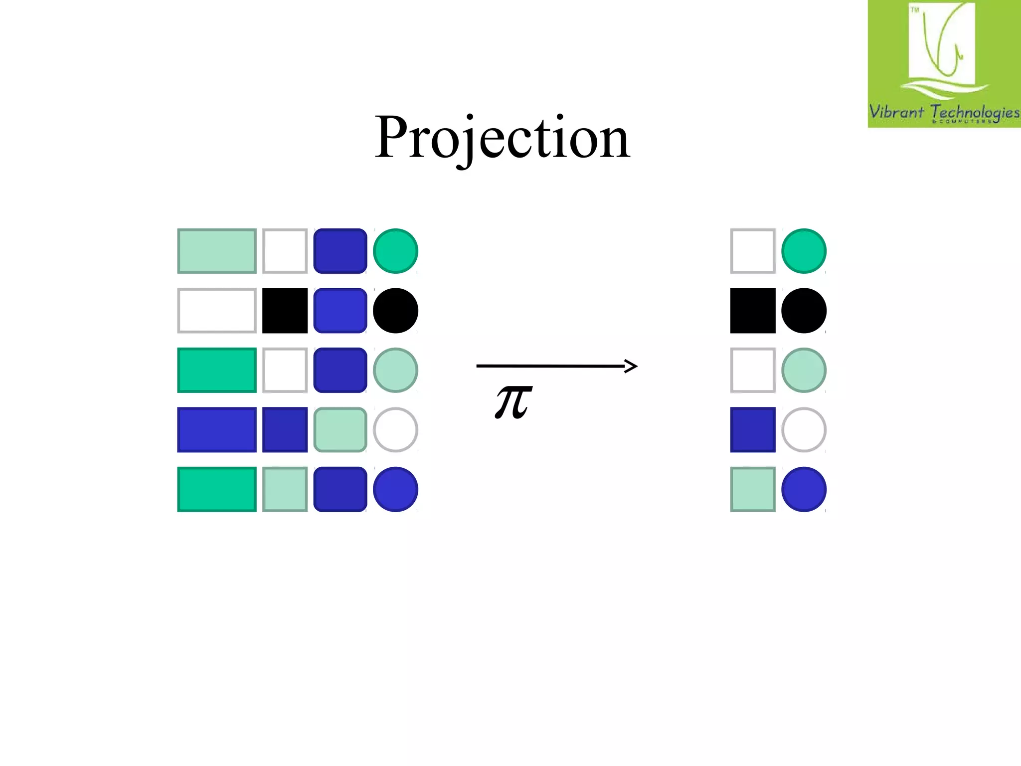
![Projection in MapReduce
• Easy!
– Map over tuples, emit new tuples with appropriate attributes
– Reduce: take tuples that appear many times and emit only one
version (duplicate elimination)
• Tuple t in R: Map(t, t) - (t’,t’)
• Reduce (t’, [t’, …,t’]) - [t’,t’]
• Basically limited by HDFS streaming speeds
– Speed of encoding/decoding tuples becomes important
– Relational databases take advantage of compression
– Semistructured data? No problem!](https://image.slidesharecdn.com/hadoopclassesinmumbai-141030043751-conversion-gate02/75/Hadoop-classes-in-mumbai-62-2048.jpg)
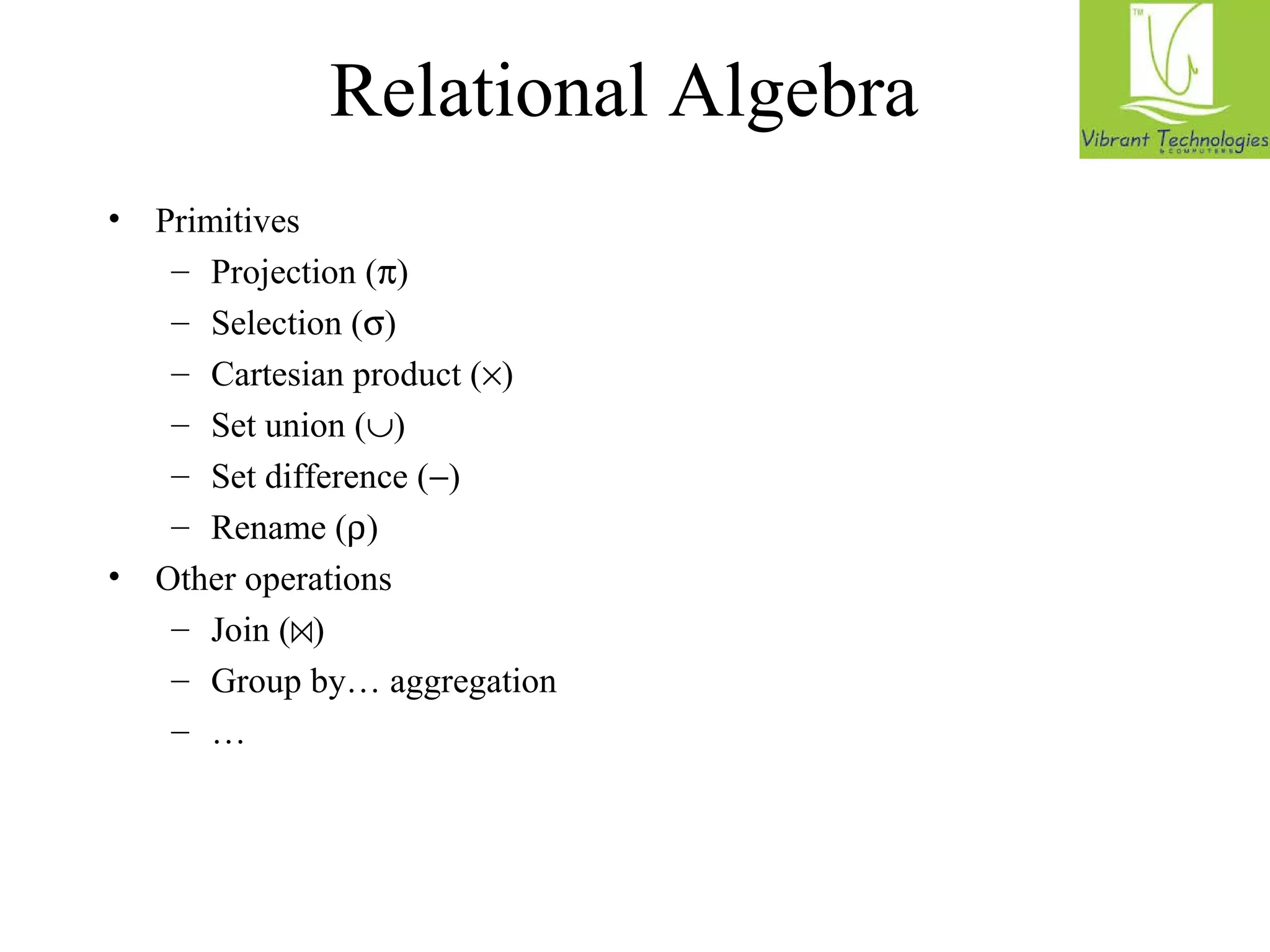
![Union, Set Intersection and Set
Difference
• Similar ideas: each map outputs the tuple
pair (t,t). For union, we output it once, for
intersection only when in the reduce we
have (t, [t,t])
• For Set difference?](https://image.slidesharecdn.com/hadoopclassesinmumbai-141030043751-conversion-gate02/75/Hadoop-classes-in-mumbai-65-2048.jpg)
![Set Difference
- Map Function: For a tuple t in R, produce key-value
pair (t, R), and for a tuple t in S, produce
key-value pair (t, S).
- Reduce Function: For each key t, do the following.
1. If the associated value list is [R], then
produce (t, t).
2. If the associated value list is anything else,
which could only be [R, S], [S, R], or [S], produce
(t, NULL).](https://image.slidesharecdn.com/hadoopclassesinmumbai-141030043751-conversion-gate02/75/Hadoop-classes-in-mumbai-66-2048.jpg)


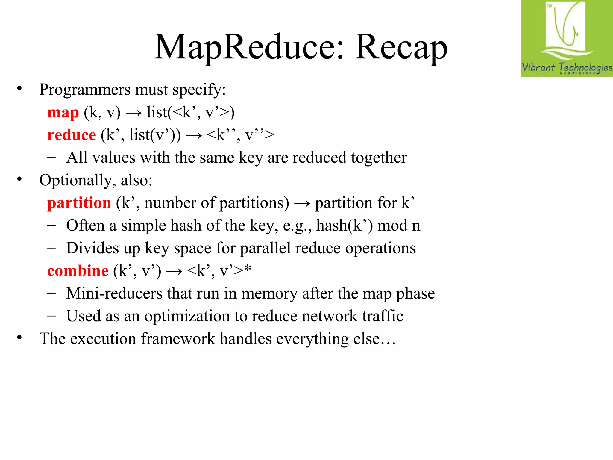
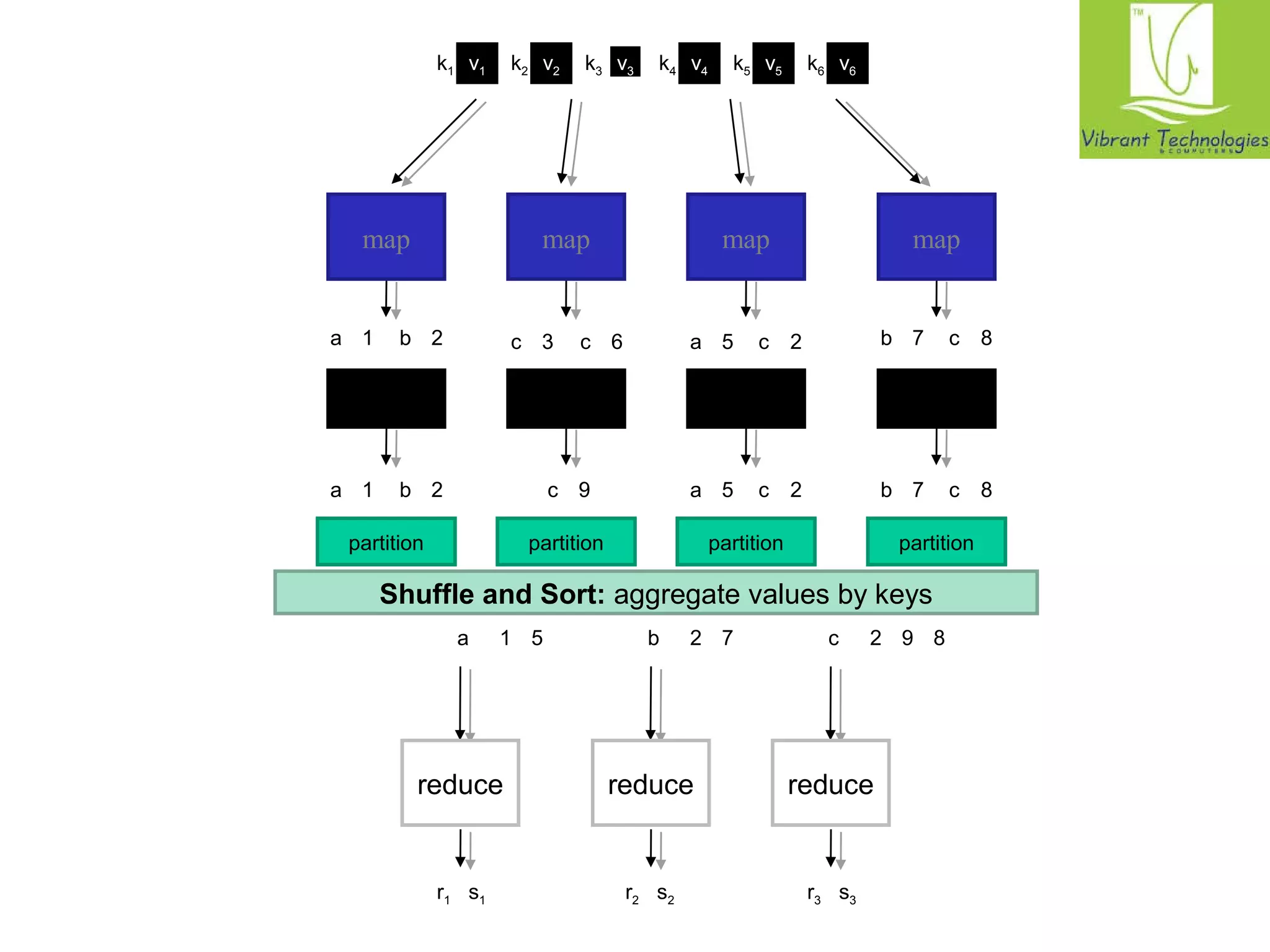
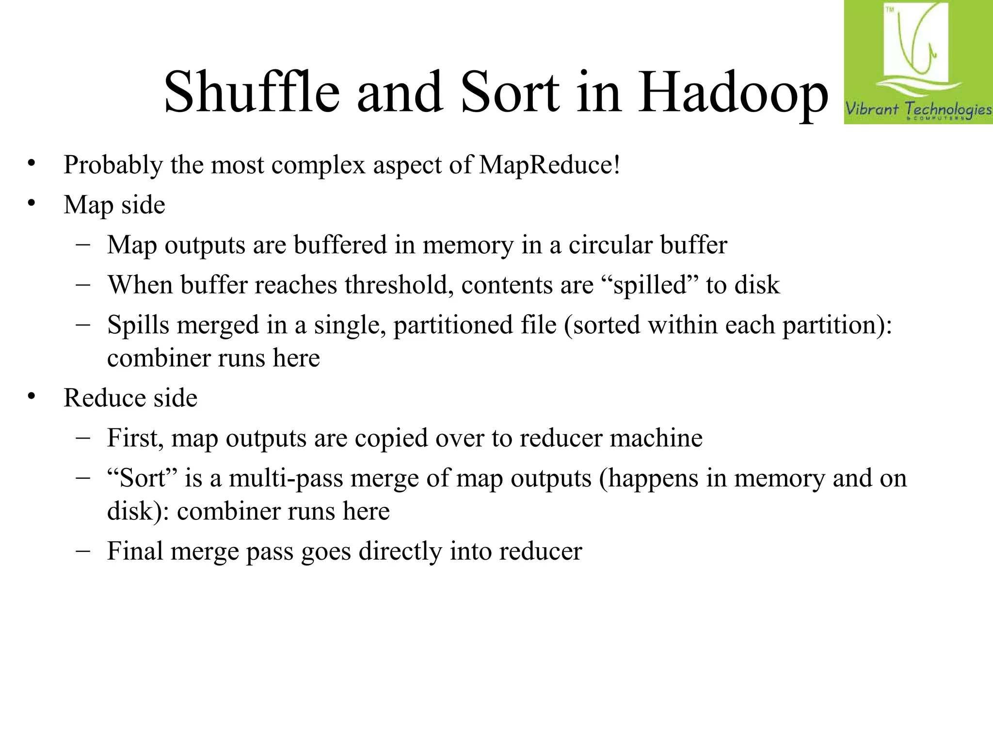
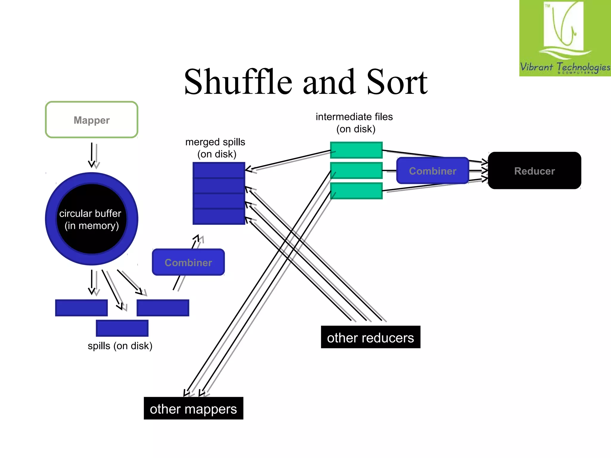
The document provides a comprehensive overview of the MapReduce programming model, specifically focusing on its application in data management and processing within Hadoop. It details the structure of MapReduce jobs, including the roles of mappers, reducers, and combiners, as well as the complexities of data synchronization, partitioning, and execution flow. Additionally, it explores graph algorithms implemented in MapReduce, with emphasis on practical examples like calculating PageRank and managing relational data operations.