Download as PDF, PPTX


![Manufacturability Status & Challenges
Dispearance
1980 1990 2000 2010 2020
10
1
0.1
um
[Courtesy Intel]
X
5 / 36](https://image.slidesharecdn.com/b22017-hsdfinal-171030091003/85/GTC-Taiwan-2017-GPU-EDA-6-320.jpg)
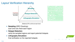
![Pattern Matching based Hotspot Detection
library'
hotspot&
Pa)ern'
matching'
hotspot&
hotspot&
detected
hotspot&
undetected
detected
Cannot&detect&
hotspots¬&in&
the&library&
Fast and accurate
[Yu+,ICCAD’14] [Nosato+,JM3’14] [Su+,TCAD’15]
Fuzzy pattern matching [Wen+,TCAD’14]
Hard to detect non-seen pattern
8 / 36](https://image.slidesharecdn.com/b22017-hsdfinal-171030091003/85/GTC-Taiwan-2017-GPU-EDA-10-320.jpg)

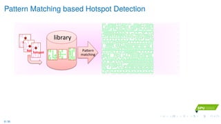
![Machine Learning based Hotspot Detection
Non$
Hotspot
Hotspot
Hotspot&
detec*on&
model&
Classifica*on&
Extract&layout&
features&
Hard,to,trade$off,
accuracy,and,false,
alarms,
Predict new patterns
Decision-tree, ANN, SVM, Boosting ...
[Drmanac+,DAC’09] [Ding+,TCAD’12] [Yu+,JM3’15] [Matsunawa+,SPIE’15] [Yu+,TCAD’15]
Hard to balance accuracy and false-alarm
9 / 36](https://image.slidesharecdn.com/b22017-hsdfinal-171030091003/85/GTC-Taiwan-2017-GPU-EDA-12-320.jpg)


![Learning Models
Support Vector Machine
[ASPDAC’12][TCAD’15]
Classifier:
Artificial Neural Network
[ASPDAC’12][JOP’13]
x1
x2
x3
h1
h2
h3
h4
y1
y2
Input Hidden Output
W1 W2
Feedforward Prediction/Regression:
Boosting
[SPIE’15][ICCAD’116]
Ensemble machine learning methods
that can build strong classifiers from a
set of weak classifiers.
Adaboost and Decision Tree:
11 / 36](https://image.slidesharecdn.com/b22017-hsdfinal-171030091003/85/GTC-Taiwan-2017-GPU-EDA-15-320.jpg)
![Conventional Feature Extraction
r
0"
0"
0"
0"
F
0"
F_In
F_Ex
F_ExIn
F_InEx
-1-2 +1 +2…
…
…
…
…
+2
-2
-1
-1 +2+1
-2+1
-1
+1
+2
-1 +1
+2
…
Fragment
[ASPDAC’12][JM3’15]
HLAC
[JM3’14]
0 order
1st order
2nd order
Density
[SPIE’15]
a11 a12 a13 a14 a15
a21 a22 a23 a24 a25
a31 a32 a33 a23 a35
a41 a42 a43 a44 a45
a51 a52 a53 a54 a55
ws
wn
12 / 36](https://image.slidesharecdn.com/b22017-hsdfinal-171030091003/85/GTC-Taiwan-2017-GPU-EDA-16-320.jpg)
![Feature Evaluation
(a) Fragment
3 2 1 0 1 2 3 43
2
1
0
1
2
3
(b) HLAC
2.5 2.0 1.5 1.0 0.5 0.0 0.5 1.0 1.5 2.02.0
1.5
1.0
0.5
0.0
0.5
1.0
1.5
2.0
(c) Density
For hotspot feature i, calculate Mahalanobis distance [Mahalanobis,1936].
di =
(xi − µ)TV−1(xi − µ) − dmin
dmax − dmin
As large as possible
13 / 36](https://image.slidesharecdn.com/b22017-hsdfinal-171030091003/85/GTC-Taiwan-2017-GPU-EDA-17-320.jpg)
![Feature Engineering Example: CCAS
Training Layout Clips Dense Circuit Sampling CCAS
Concentric Circle Area Sampling (CCAS) [Matsunawa+,JM3’16].
Capture the affects of light diffraction.
Simple rule to select circles from dense samples.
14 / 36](https://image.slidesharecdn.com/b22017-hsdfinal-171030091003/85/GTC-Taiwan-2017-GPU-EDA-18-320.jpg)
![Feature Engineering Example: CCAS
Training Layout Clips Dense Circuit Sampling CCAS
Concentric Circle Area Sampling (CCAS) [Matsunawa+,JM3’16].
Capture the affects of light diffraction.
Simple rule to select circles from dense samples.
Question:
Can we find correlation between circles and hotspots, and select circles smartly?
14 / 36](https://image.slidesharecdn.com/b22017-hsdfinal-171030091003/85/GTC-Taiwan-2017-GPU-EDA-19-320.jpg)
![Smart CCAS Circle Selection [ICCAD’16]
Higer Mutual Information, more correlation between circle and label variable.
0
0.1
0.2
0.3
0.4
0.5
0.6
0.7
0.8
0 100 200 300 400 500 600
MutualInformation
Circle Radius
Case1
Case2
Case3
1 nm
600nm
…
…
15 / 36](https://image.slidesharecdn.com/b22017-hsdfinal-171030091003/85/GTC-Taiwan-2017-GPU-EDA-20-320.jpg)
![Smart CCAS Circle Selection [ICCAD’16]
Mathematical Formulation
max
w
v w
s.t. vi = I(Ci; Y), ∀vi ∈ v,
||w||0 = nc, ∀ i, wi ∈ {0, 1},
|i − j| ≥ d, ∀ i = j, wi = wj = 1.
0
0.1
0.2
0.3
0.4
0.5
0.6
0.7
0.8
0 100 200 300 400 500 600
MutualInformation
Circle Radius
Case1
Case2
Case3
16 / 36](https://image.slidesharecdn.com/b22017-hsdfinal-171030091003/85/GTC-Taiwan-2017-GPU-EDA-21-320.jpg)
![Smart CCAS Circle Selection [ICCAD’16]
Mathematical Formulation
max
w
v w
s.t. vi = I(Ci; Y), ∀vi ∈ v,
||w||0 = nc, ∀ i, wi ∈ {0, 1},
|i − j| ≥ d, ∀ i = j, wi = wj = 1.
0
0.1
0.2
0.3
0.4
0.5
0.6
0.7
0.8
0 100 200 300 400 500 600
MutualInformation
Circle Radius
Case1
Case2
Case3
Optimally Solved by Dynamic Programming
D[i, j] = max{v[i] + D[i − d, j − 1], D[i − 1, j]}},
D[i, j]: optimal solution from range {1, i}, when totally j circles are selected.
16 / 36](https://image.slidesharecdn.com/b22017-hsdfinal-171030091003/85/GTC-Taiwan-2017-GPU-EDA-22-320.jpg)

![Why Deep Learning?
Feature Crafting v.s. Feature Learning
Although prior knowledge is considered during manually feature design, information
loss is inevitable. Feature learned from mass dataset is more reliable.
Scalability
With shrinking down circuit feature size, mask layout becomes more complicated.
Deep learning has the potential to handle ultra-large-scale instances while traditional
machine learning may suffer from performance degradation.
Mature Libraries
Caffe [Jia+,ACMMM’14] and Tensorflow [Martin+,TR’15]
Powerful GPU for training
17 / 36](https://image.slidesharecdn.com/b22017-hsdfinal-171030091003/85/GTC-Taiwan-2017-GPU-EDA-24-320.jpg)
![Architecture Summary [SPIE’17]
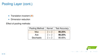
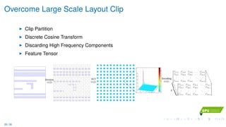
Total 21 layers with 13 convolution layers and 5 pooling layers.
A ReLU is applied after each convolution layer.
…
…
Hotspot
Non-Hotspot
512x512x4
256x256x4
256x256x8
128x128x16
128x128x8
64x64x16
64x64x32
32x32x32 32x32x32
16x16x32
2048
512
C1-1
C1-2 C2-1C2-2 C2-3
P2 C3-1 C3-2
C4-1P3C3-3 C4-2 C4-3
C5-1 C5-2 C5-3P4 P5
24 / 36](https://image.slidesharecdn.com/b22017-hsdfinal-171030091003/85/GTC-Taiwan-2017-GPU-EDA-31-320.jpg)
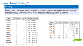
![Architecture Summary [SPIE’17]
Layer Kernel Size Stride Padding Output Vertexes
Conv1-1 2 × 2 × 4 2 0 512 × 512 × 4
Pool1 2 × 2 2 0 256 × 256 × 4
Conv2-1 3 × 3 × 8 1 1 256 × 256 × 8
Conv2-2 3 × 3 × 8 1 1 256 × 256 × 8
Conv2-3 3 × 3 × 8 1 1 256 × 256 × 8
Pool2 2 × 2 2 0 128 × 128 × 8
Conv3-1 3 × 3 × 16 1 1 128 × 128 × 16
Conv3-2 3 × 3 × 16 1 1 128 × 128 × 16
Conv3-3 3 × 3 × 16 1 1 128 × 128 × 16
Pool3 2 × 2 2 0 64 × 64 × 16
Conv4-1 3 × 3 × 32 1 1 64 × 64 × 32
Conv4-2 3 × 3 × 32 1 1 64 × 64 × 32
Conv4-3 3 × 3 × 32 1 1 64 × 64 × 32
Pool4 2 × 2 2 0 32 × 32 × 32
Conv5-1 3 × 3 × 32 1 1 32 × 32 × 32
Conv5-2 3 × 3 × 32 1 1 32 × 32 × 32
Conv5-3 3 × 3 × 32 1 1 32 × 32 × 32
Pool5 2 × 2 2 0 16 × 16 × 32
FC1 – – – 2048
FC2 – – – 512
FC3 – – – 2
25 / 36](https://image.slidesharecdn.com/b22017-hsdfinal-171030091003/85/GTC-Taiwan-2017-GPU-EDA-32-320.jpg)
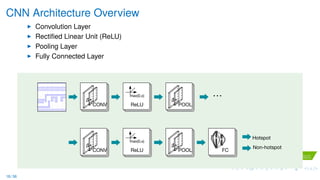
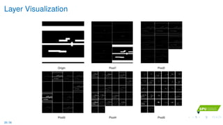
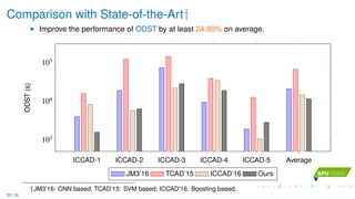
![Simplified CNN Architecture [DAC’17]
Feature Tensor
k-channel hyper-image
Compatible with CNN
Storage and computional efficiency
Layer Kernel Size Stride Output Node #
conv1-1 3 1 12 × 12 × 16
conv1-2 3 1 12 × 12 × 16
maxpooling1 2 2 6 × 6 × 16
conv2-1 3 1 6 × 6 × 32
conv2-2 3 1 6 × 6 × 32
maxpooling2 2 2 3 × 3 × 32
fc1 N/A N/A 250
fc2 N/A N/A 2
…
Hotspot
Non-Hotspot
Convolution + ReLU Layer Max Pooling Layer Full Connected Node
2
6
6
6
4
C11,1 C12,1 C13,1 . . . C1n,1
C21,1 C22,1 C23,1 . . . C2n,1
...
...
...
...
...
Cn1,1 Cn2,1 Cn3,1 . . . Cnn,1
3
7
7
7
5
2
6
6
6
4
C11,k C12,k C13,k . . . C1n,k
C21,k C22,k C23,k . . . C2n,k
...
...
...
...
...
Cn1,k Cn2,k Cn3,k . . . Cnn,k
3
7
7
7
5
(
k
27 / 36](https://image.slidesharecdn.com/b22017-hsdfinal-171030091003/85/GTC-Taiwan-2017-GPU-EDA-34-320.jpg)


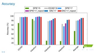
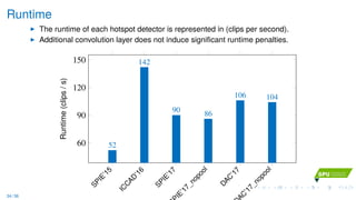


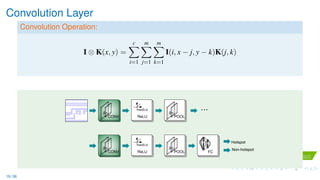
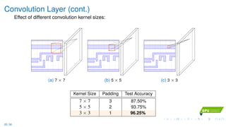
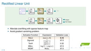
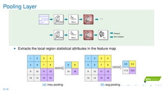
A deep learning model using convolutional neural networks is proposed for lithography hotspot detection. The model takes layout clip images as input and outputs a prediction of hotspot or non-hotspot. It uses several convolutional and pooling layers to automatically learn features from the images without manual feature engineering. Evaluation shows the deep learning model achieves higher accuracy than previous shallow learning methods that rely on manually designed features.