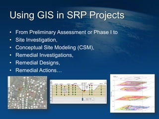
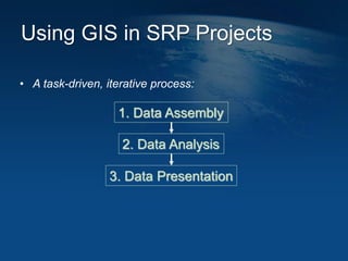
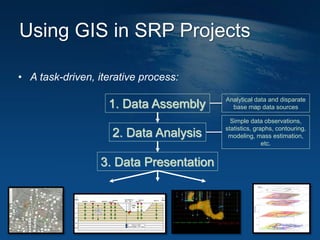
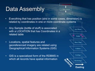
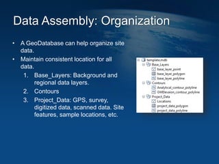
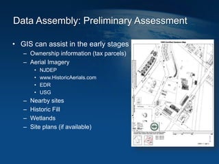
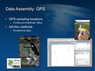
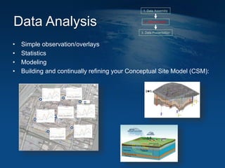
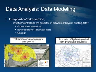
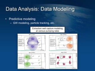
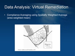
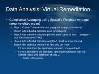
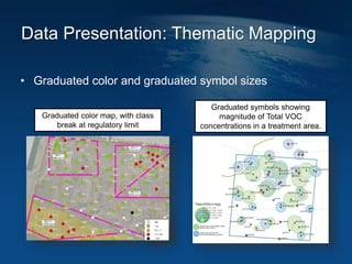
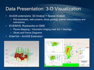
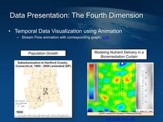
GIS ANALYSIS AND WORK-
PRODUCTS SUPPORTING SRP
The Application of Geographic Information Systems (GIS) to
the Site Remediation Program – An Introduction
Joe Luchette:
jluchette@geosyntec.com
Using GIS in SRP Projects
• From Preliminary Assessment or Phase I to
• Site Investigation,
• Conceptual Site Modeling (CSM),
• Remedial Investigations,
• Remedial Designs,
• Remedial Actions…
• A task-driven, iterative process:
1. Data Assembly
2. Data Analysis
3. Data Presentation
Using GIS in SRP Projects
• A task-driven, iterative process:
1. Data Assembly
2. Data Analysis
3. Data Presentation
Analytical data and disparate
base map data sources
Simple data observations,
statistics, graphs, contouring,
modeling, mass estimation,
etc.
Using GIS in SRP Projects
Data Assembly
• Everything that has position (and in some cases, dimension) is
related by coordinates in one or more coordinate systems
Air Photo
Base Map
Utilities
Wells
Geology
Hydrology
Easting
• Any Sample (bottle of stuff) is associated
with a LOCATION that has Coordinates in a
related table
• Locations, spatial features and
georeferenced imagery are related using
Geographical Information Systems (GIS)
• GIS is a specialized form of the RDBMS in
which all records have spatial information
1. Data Assembly
2. Data Analysis
3. Data Presentation
Data Assembly: Organization
• A GeoDatabase can help organize site
data.
• Maintain consistent location for all
data.
1. Base_Layers: Background and
regional data layers.
2. Contours
3. Project_Data: GPS, survey,
digitized data, scanned data. Site
features, sample locations, etc.
Data Assembly: Preliminary Assessment
• GIS can assist in the early stages
– Ownership information (tax parcels)
– Aerial Imagery
• NJDEP
• www.HistoricAerials.com
• EDR
• USG
– Nearby sites
– Historic Fill
– Wetlands
– Site plans (if available)
• Conversion is not necessarily transitive:
cannot always reproduce the original CAD
data after converting to GIS due to inherent
differences in CAD/GIS data models
• Tips for requesting DWGs:
– Use model space
– Explode blocks,
– Don’t use mtext,
– Don’t use hatching,
– Organize layers well
Data Assembly: Working with AutoCAD Drawings
Traditionally Doesn’t interface well with GIS.
Data Assembly: Working with AutoCAD Drawings
• Bi-directional conversions between CAD
and GIS data
– Use ArcToolbox to convert CAD to GIS
& GIS to CAD
• ArcToolbox > Conversion Tools>To
Geodatabase > Import from CAD
• ArcToolbox > Conversion Tools>To
CAD>Export to CAD
Data Assembly: GeoReferencing
• GeoReferencing
– Digitizing
– Raster to Vector Conversion (ArcScan)
Vectorization of contours
using ArcScan
GeoReferencing a drawing
onto an aerial
Data Assembly: GPS
• GPS sampling locations
– Trimble and Pathfinder Office
• Ad-Hoc methods
– Smartphone Apps
Data Analysis
• Simple observation/overlays
• Statistics
• Modeling
• Building and continually refining your Conceptual Site Model (CSM):
1. Data Assembly
2. Data Analysis
3. Data Presentation
MW-
114
MW-
116
MW-
118
MW-
117
MW-
113
MW-
115
MW-
119
Data Analysis: Overlay
• Data Observation:
– Historic imagery overlays
– Topographic overlays
– Site plan overlays- historic use
Data Analysis: Data Modeling
• Interpolation/extrapolation,
– What concentrations are expected in between or beyond existing data?
• Groundwater elevations
• Isoconcentration (analytical data)
• Geology
TCE isoconcentration contours
with color fill
Interpolation of hydraulic gradient
from groundwater elevations
Data Analysis: Data Modeling
• Predictive modeling
– GW modeling, particle tracking, etc.
Extraction well capture modeling
at various pumping rates
Data Analysis: Virtual Remediation
• Compliance Averaging using Spatially Weighted Average
(area weighted mean)
Data Analysis: Virtual Remediation
• Compliance Averaging using Spatially Weighted Average
(area weighted mean)
– Step 1: Create Thiessen/Voronoi polygons from points dataset.
– Step 2: Add a field & calculate area for polygons
– Step 3: Add a field & calculate percent area ((area of each polygon ÷
total functional area)*100)
– Step 4: Add a field & calculate weighted result for a compound
– Step 5: Get statistics on the final field and get mean
• If this is less than the applicable standard, you are done!
• If this is still above the standard, take out the polygon with the
highest result, and start over at step 2.
– Iterate until complete.
Data Presentation
• You are telling a story through narratives, tables, charts, maps and
other visualizations
• Maps are fundamental to environmental data to communicate spatial
component
• Yes, every picture tells a story (in fact, most pictures tell several
stories), but the key is finding THE picture…
1. Data Assembly
2. Data Analysis
3. Data Presentation
“There’s no such thing as an objective map”
--Michael Goodchild
Data Presentation: Thematic Mapping
• Graduated color and graduated symbol sizes
Graduated symbols showing
magnitude of Total VOC
concentrations in a treatment area.
Graduated color map, with class
break at regulatory limit
Data Presentation: Thematic Mapping
• Pie Charts and Graph maps
Time-series concentration data
suggest transport of vinyl chloride is
to the west, off-site.
Pie charts showing compound ratios
in Total VOC summations.
Data Presentation: Data Posting
• Advanced Labeling (aka “Spider Maps” or “Data Box Maps”)
– Show multiple samples (depth, dates)
– Highlight results above standards
– Use in combination with symbology
Data Presentation: Leaving Plan View
• GIS provides a quick start to your Cross Sections
– Use the X or Y coordinate as the X axis, and use the elevation or depth
measurements and use at as the Y axis to start constructing your
scaled graphic.
– Add your labels
– Draw in your contacts
Data Presentation: Leaving Plan View
• Psuedo 3-D
– Showing Depth using planar maps
Juxtaposition Stacking
Data Presentation: 3-D Visualization
• ArcGIS extensions: 3D Analyst + Spatial Analyst
– Plot boreholes, well screens, block geology (planar interpolations and
extrusions)
• EVS/MVS, Rockworks or GMS
– Plume Mapping - Volumetric Kriging (real 3d) + Geology
– Slices and Fence Diagrams
• EnterVol – ArcGIS Extension
Data Presentation: The Fourth Dimension
• Temporal Data Visualization using Animation
– Stream Flow animation with corresponding graph: Link
Modeling Nutrient Delivery in a
Bioremediation Curtain
Population Growth
www.egr.msu.edu
Helpful Links
• State of NJ – Tax List Search: http://njgin.state.nj.us/oit/gis/NJ_TaxListSearch
• NJDEP Compliance Averaging Guidance:
www.nj.gov/dep/srp/guidance/srra/attainment_compliance.pdf
• Golden Software - Surfer: http://www.goldensoftware.com/products/surfer
• ArcGIS – 3D Analyst Extension:
http://www.esri.com/software/arcgis/extensions/3danalyst
• ArcGIS – Spatial Analyst Extension:
http://www.esri.com/software/arcgis/extensions/spatialanalyst
• Ctech – EVS/MVS Suite: http://www.ctech.com/mvsevs-product-suite-new/
• EnterVol – EVS ArcGIS extension: http://entervol.com/
• Visualizing Temporal data in ArcGIS:
http://resources.arcgis.com/en/help/main/10.1/index.html#/About_visualizing_t
emporal_data/005z0000000n000000/
QUESTION AND ANSWER
GIS analysis and work-products supporting SRP

GIS Analysis For Site Remediation

  • 1.
    GIS ANALYSIS ANDWORK- PRODUCTS SUPPORTING SRP The Application of Geographic Information Systems (GIS) to the Site Remediation Program – An Introduction Joe Luchette: jluchette@geosyntec.com
  • 2.
    Using GIS inSRP Projects • From Preliminary Assessment or Phase I to • Site Investigation, • Conceptual Site Modeling (CSM), • Remedial Investigations, • Remedial Designs, • Remedial Actions…
  • 3.
    • A task-driven,iterative process: 1. Data Assembly 2. Data Analysis 3. Data Presentation Using GIS in SRP Projects
  • 4.
    • A task-driven,iterative process: 1. Data Assembly 2. Data Analysis 3. Data Presentation Analytical data and disparate base map data sources Simple data observations, statistics, graphs, contouring, modeling, mass estimation, etc. Using GIS in SRP Projects
  • 5.
    Data Assembly • Everythingthat has position (and in some cases, dimension) is related by coordinates in one or more coordinate systems Air Photo Base Map Utilities Wells Geology Hydrology Easting • Any Sample (bottle of stuff) is associated with a LOCATION that has Coordinates in a related table • Locations, spatial features and georeferenced imagery are related using Geographical Information Systems (GIS) • GIS is a specialized form of the RDBMS in which all records have spatial information 1. Data Assembly 2. Data Analysis 3. Data Presentation
  • 6.
    Data Assembly: Organization •A GeoDatabase can help organize site data. • Maintain consistent location for all data. 1. Base_Layers: Background and regional data layers. 2. Contours 3. Project_Data: GPS, survey, digitized data, scanned data. Site features, sample locations, etc.
  • 7.
    Data Assembly: PreliminaryAssessment • GIS can assist in the early stages – Ownership information (tax parcels) – Aerial Imagery • NJDEP • www.HistoricAerials.com • EDR • USG – Nearby sites – Historic Fill – Wetlands – Site plans (if available)
  • 8.
    • Conversion isnot necessarily transitive: cannot always reproduce the original CAD data after converting to GIS due to inherent differences in CAD/GIS data models • Tips for requesting DWGs: – Use model space – Explode blocks, – Don’t use mtext, – Don’t use hatching, – Organize layers well Data Assembly: Working with AutoCAD Drawings Traditionally Doesn’t interface well with GIS.
  • 9.
    Data Assembly: Workingwith AutoCAD Drawings • Bi-directional conversions between CAD and GIS data – Use ArcToolbox to convert CAD to GIS & GIS to CAD • ArcToolbox > Conversion Tools>To Geodatabase > Import from CAD • ArcToolbox > Conversion Tools>To CAD>Export to CAD
  • 10.
    Data Assembly: GeoReferencing •GeoReferencing – Digitizing – Raster to Vector Conversion (ArcScan) Vectorization of contours using ArcScan GeoReferencing a drawing onto an aerial
  • 11.
    Data Assembly: GPS •GPS sampling locations – Trimble and Pathfinder Office • Ad-Hoc methods – Smartphone Apps
  • 12.
    Data Analysis • Simpleobservation/overlays • Statistics • Modeling • Building and continually refining your Conceptual Site Model (CSM): 1. Data Assembly 2. Data Analysis 3. Data Presentation MW- 114 MW- 116 MW- 118 MW- 117 MW- 113 MW- 115 MW- 119
  • 13.
    Data Analysis: Overlay •Data Observation: – Historic imagery overlays – Topographic overlays – Site plan overlays- historic use
  • 14.
    Data Analysis: DataModeling • Interpolation/extrapolation, – What concentrations are expected in between or beyond existing data? • Groundwater elevations • Isoconcentration (analytical data) • Geology TCE isoconcentration contours with color fill Interpolation of hydraulic gradient from groundwater elevations
  • 15.
    Data Analysis: DataModeling • Predictive modeling – GW modeling, particle tracking, etc. Extraction well capture modeling at various pumping rates
  • 16.
    Data Analysis: VirtualRemediation • Compliance Averaging using Spatially Weighted Average (area weighted mean)
  • 17.
    Data Analysis: VirtualRemediation • Compliance Averaging using Spatially Weighted Average (area weighted mean) – Step 1: Create Thiessen/Voronoi polygons from points dataset. – Step 2: Add a field & calculate area for polygons – Step 3: Add a field & calculate percent area ((area of each polygon ÷ total functional area)*100) – Step 4: Add a field & calculate weighted result for a compound – Step 5: Get statistics on the final field and get mean • If this is less than the applicable standard, you are done! • If this is still above the standard, take out the polygon with the highest result, and start over at step 2. – Iterate until complete.
  • 18.
    Data Presentation • Youare telling a story through narratives, tables, charts, maps and other visualizations • Maps are fundamental to environmental data to communicate spatial component • Yes, every picture tells a story (in fact, most pictures tell several stories), but the key is finding THE picture… 1. Data Assembly 2. Data Analysis 3. Data Presentation “There’s no such thing as an objective map” --Michael Goodchild
  • 19.
    Data Presentation: ThematicMapping • Graduated color and graduated symbol sizes Graduated symbols showing magnitude of Total VOC concentrations in a treatment area. Graduated color map, with class break at regulatory limit
  • 20.
    Data Presentation: ThematicMapping • Pie Charts and Graph maps Time-series concentration data suggest transport of vinyl chloride is to the west, off-site. Pie charts showing compound ratios in Total VOC summations.
  • 21.
    Data Presentation: DataPosting • Advanced Labeling (aka “Spider Maps” or “Data Box Maps”) – Show multiple samples (depth, dates) – Highlight results above standards – Use in combination with symbology
  • 22.
    Data Presentation: LeavingPlan View • GIS provides a quick start to your Cross Sections – Use the X or Y coordinate as the X axis, and use the elevation or depth measurements and use at as the Y axis to start constructing your scaled graphic. – Add your labels – Draw in your contacts
  • 23.
    Data Presentation: LeavingPlan View • Psuedo 3-D – Showing Depth using planar maps Juxtaposition Stacking
  • 24.
    Data Presentation: 3-DVisualization • ArcGIS extensions: 3D Analyst + Spatial Analyst – Plot boreholes, well screens, block geology (planar interpolations and extrusions) • EVS/MVS, Rockworks or GMS – Plume Mapping - Volumetric Kriging (real 3d) + Geology – Slices and Fence Diagrams • EnterVol – ArcGIS Extension
  • 25.
    Data Presentation: TheFourth Dimension • Temporal Data Visualization using Animation – Stream Flow animation with corresponding graph: Link Modeling Nutrient Delivery in a Bioremediation Curtain Population Growth www.egr.msu.edu
  • 26.
    Helpful Links • Stateof NJ – Tax List Search: http://njgin.state.nj.us/oit/gis/NJ_TaxListSearch • NJDEP Compliance Averaging Guidance: www.nj.gov/dep/srp/guidance/srra/attainment_compliance.pdf • Golden Software - Surfer: http://www.goldensoftware.com/products/surfer • ArcGIS – 3D Analyst Extension: http://www.esri.com/software/arcgis/extensions/3danalyst • ArcGIS – Spatial Analyst Extension: http://www.esri.com/software/arcgis/extensions/spatialanalyst • Ctech – EVS/MVS Suite: http://www.ctech.com/mvsevs-product-suite-new/ • EnterVol – EVS ArcGIS extension: http://entervol.com/ • Visualizing Temporal data in ArcGIS: http://resources.arcgis.com/en/help/main/10.1/index.html#/About_visualizing_t emporal_data/005z0000000n000000/
  • 27.
    QUESTION AND ANSWER GISanalysis and work-products supporting SRP