Download as PDF, PPTX


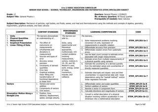
![GENERAL PHYSICS 1
QUARTER 1
Units, Physical Quantities, Measurement, Errors and Uncertainties, Graphical Presentation, & Linear Fitting of
Data
GP1-01-17
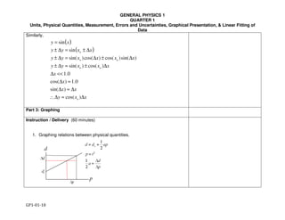
∆≈∆
∆
∆
≈
= oxxdx
df
xf
x
f
dx
df
( )
[ ]
)cos(
)sin(
sin
o
xx
o
xxy
x
dx
d
xy
xxx
xy
o
∆≈∆
∆≈∆
∆±=
=
=
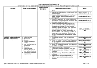
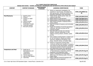
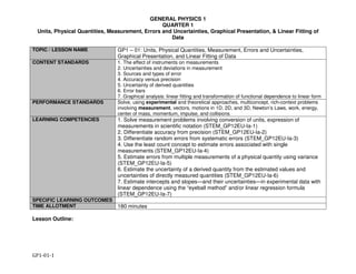
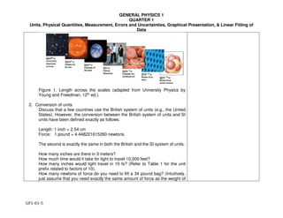
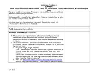
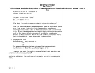
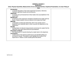
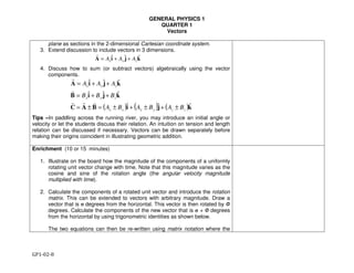
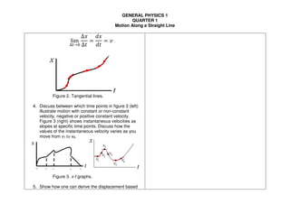
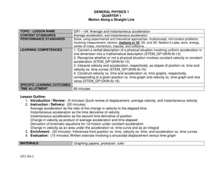
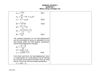
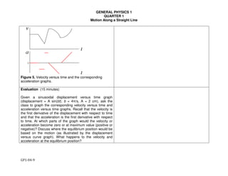
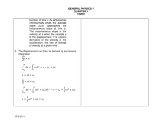
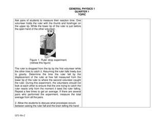
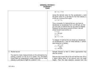
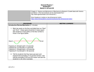
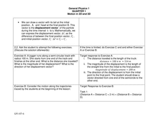
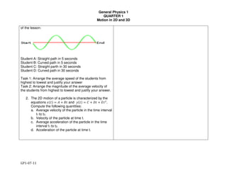
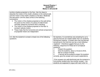
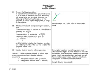
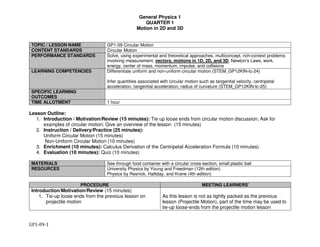
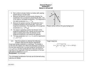
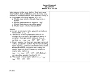
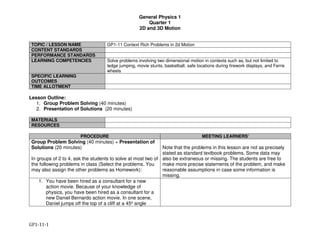
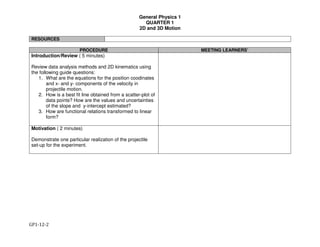
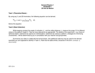
Figure 2. Function of one variable and its error Δf. Given a function f(x), the local
slope at xo is calculated as the first derivative at xo.
Example:](https://image.slidesharecdn.com/physics1initialreleasejune13-160615223814/85/GENERAL-PHYSICS-1-TEACHING-GUIDE-35-320.jpg)
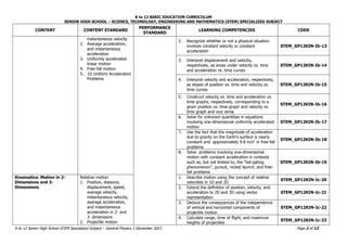
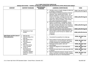
![General Physics 1
QUARTER 1
Motion in 2D and 3D
GP1-07-10
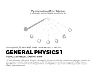
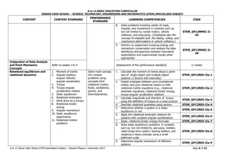
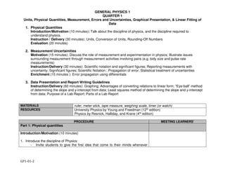
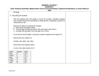
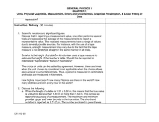
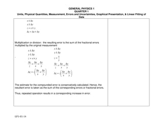
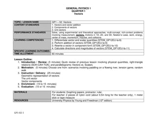
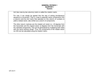
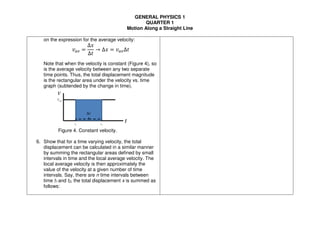
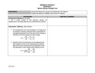
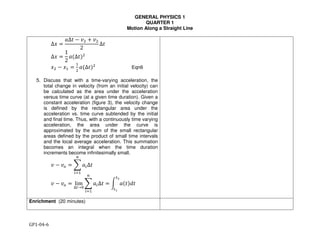
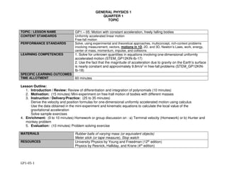
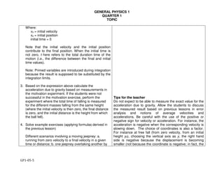
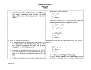
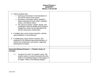
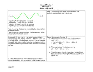
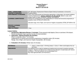
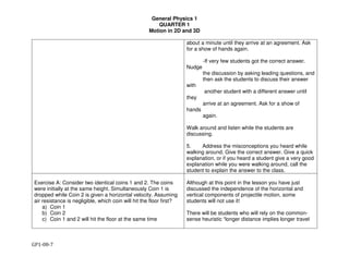
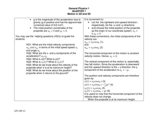
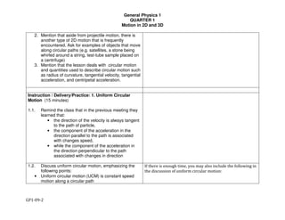
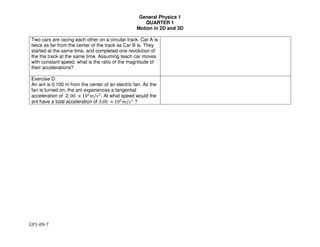
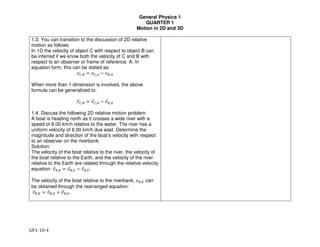
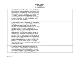
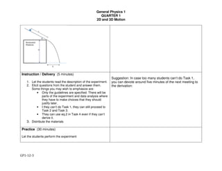
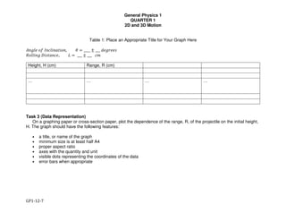
Exercise D: A jogger runs along a semi-circular track with
radius 100 m for 3.00 minutes. She starts from one end of
the track and finishes at the other end. What is her average
speed? What is the magnitude of her average velocity?
Target response for Exercise D:
!"#$!%# "#$$% =
%'"()*+$ (,)-$..$%
('/$ $.)#"$%
=
100 2
180
/
"
= 1.75 %/'
%()*+,-./ 01 (2/3()/ 2/405+,6 = |29:;;;;;;<| = =
∆3<
∆,
= =
|∆3<|
∆,
=
%()*+,-./ 01 .+'?4(5/%/*,
,+%/ /4(?'/.
=
200
180
%
'
= 1.11
%
'
Exercise E: The position of a particle in 3-dimensions is
given by
D = cosH2I,J , 6 = sinH2I,J , N = ,
where x, y,and z are in meters while t is in seconds.
Determine the following quantities:
a) Position vector at , = 0 (*. , = 1/3 s
b) Average velocity in the time interval , = 0 ,0 , =
P
Q
s
c) Instantaneous velocity at time t=0 s
d) Instantaneous velocity at time 1/3 s
e) Average acceleration in the time interval , = 0 s to
, = 1/3 s
f) Instantaneous acceleration at time t= 1.0 s
Target response:
a) 3< H0J = 1 % R̂, 3< T
P
Q
'U =
V
W
% R̂ +
√Q
W
% Ẑ +
P
Q
% [
b) 29:;;;;;;< =
∆]<
∆^
= T−
Q
W
R̂ +
Q√Q
W
Ẑ + I [U %/'
c) 2<H,J =
`
`^
acosH2I,J R̂ + sinH2I,J Ẑ + , [b
= −2π sinH2I,J R̂ + 2I cosH2I,J Ẑ + [
∴ 2<H0 'J = e2I Ẑ + [f %/'
d) 2< T
V
Q
'U = g−2π sin T
WP
Q
U R̂ + 2I cos T
WP
Q
U Ẑ + [h
i
j
= a −√3π R̂ − I Ẑ + [b
%
'
e) (9:;;;;;;< =
∆:;<
∆^
= e −3√3π R̂ − 8I Ẑf %/'
f) (<H,J =
`
`^
2<H,J = −4IWHcosH2I,J R̂ + sinH2I,J ẐJ
∴ (<H1 'J = −4 IW
R̂ %/'W
Evaluation (10 minutes)
1. Consider the motion of the four students at the beginning
In case there is not enough time, ask only Item 1 Task 2
and Item 2a & 2d](https://image.slidesharecdn.com/physics1initialreleasejune13-160615223814/85/GENERAL-PHYSICS-1-TEACHING-GUIDE-92-320.jpg)


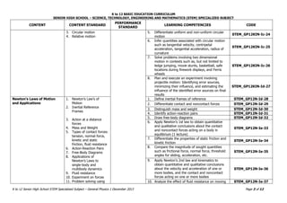
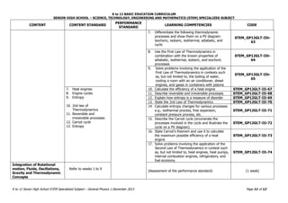
![General Physics 1
QUARTER 1
Motion in 2D and 3D
GP1-09-6
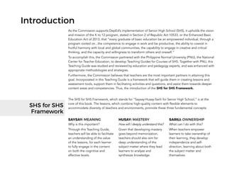
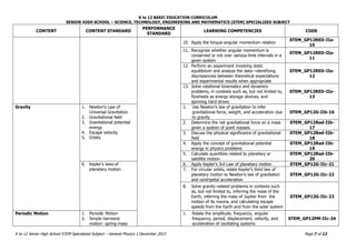
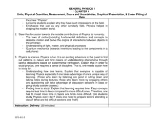
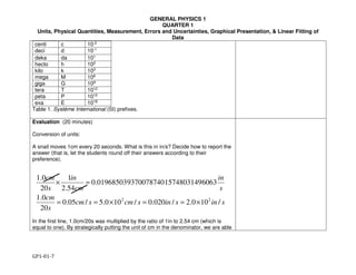
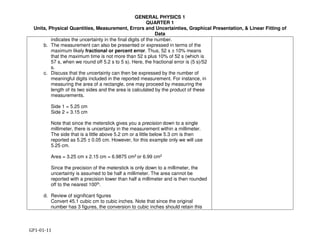
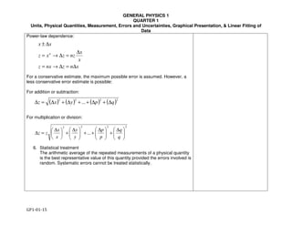
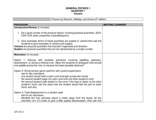
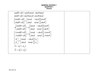
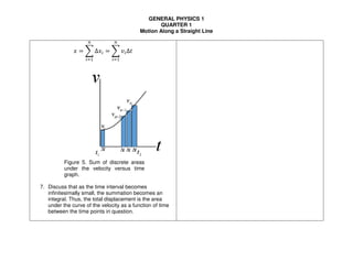
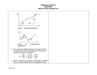
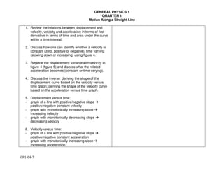
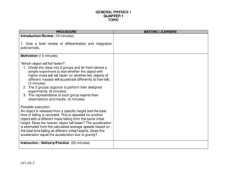
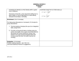
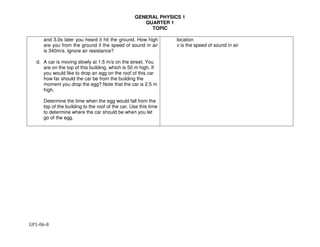
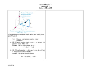
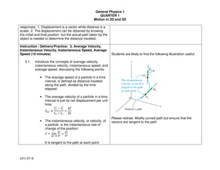
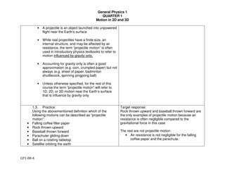
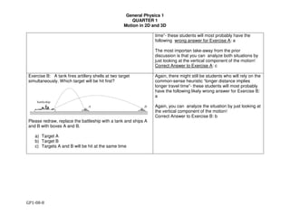
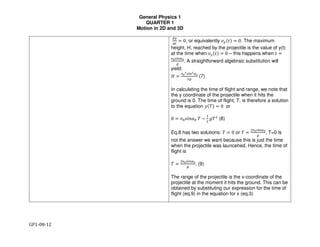
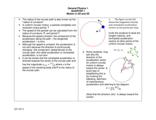
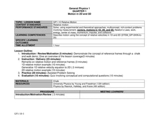
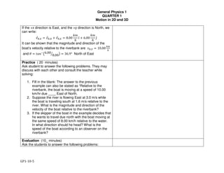
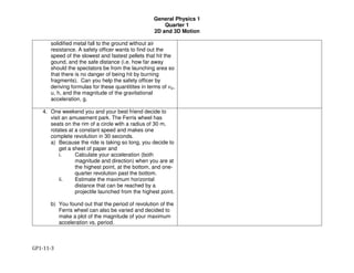
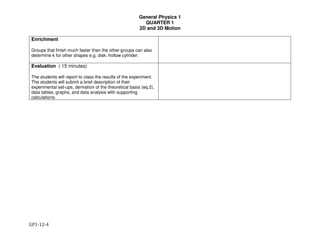
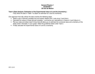
1)Consider an object moving with constant speed v along
a circular path with radius R (Uniform Circular Motion). For
simplicity let’s locate the origin of our coordinate system at
the origin, and consider a counterclockwise motion. We
will assume that y=0 at time t=0. The position vector of the
object as a function of time is
!"#$% & '()*#+$%,̂ . '*/0#+$%1̂ where + & 2/"
2)Show (or let the students show) by taking time
derivatives, that the velocity and acceleration vectors are
given by
#$%&' = −*"+,-%*&'.̂ + *"12+%*&'3̂
and
4$%&' = −*5
["12+%*&'.̂ + "+,-%*&'3]8
3) Show that the magnitude of the acceleration is given by
4 = "*5
= #5
"9
4) Verify that the acceleration and velocity vectors are
always perpendicular by showing that the dot product is
zero: 4$ ∙ #$ = 0
Evaluation (10 minutes)
Ask for a written solution to one of the following questions
or a similar question:
Exercise C:](https://image.slidesharecdn.com/physics1initialreleasejune13-160615223814/85/GENERAL-PHYSICS-1-TEACHING-GUIDE-112-320.jpg)

This document provides an overview of a Teaching Guide for a General Physics 1 course for senior high school. It outlines the course content standards and performance standards, which are mapped to specific learning competencies. The course covers units, measurement, vectors, one-dimensional kinematics including uniformly accelerated motion, and two-dimensional and three-dimensional motion. The Teaching Guide is designed to be highly usable for teachers, providing classroom activities and notes to help develop students' understanding, mastery, and ownership of the content.