Flood Routing using Muskingum Method
•Download as DOCX, PDF•
6 likes•2,960 views

It is problem related to stream flow routing using Muskingum Method.

Recommended
More Related Content
What's hot
What's hot (20)
Viewers also liked
Viewers also liked (10)
Similar to Flood Routing using Muskingum Method
Similar to Flood Routing using Muskingum Method (20)
Recently uploaded
Recently uploaded (20)
Flood Routing using Muskingum Method
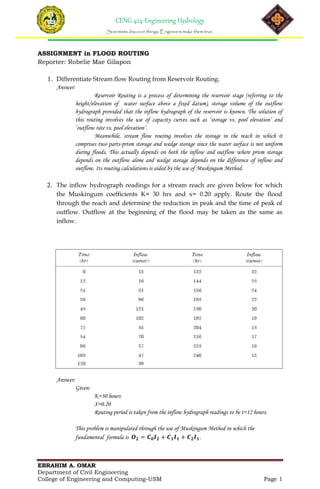
- 1. CENG 424-Engineering Hydrology Scientists discover things. Engineers make them true. EBRAHIM A. OMAR Department of Civil Engineering College of Engineering and Computing-USM Page 1 ASSIGNMENT in FLOOD ROUTING Reporter: Robelie Mae Gilapon 1. Differentiate Stream flow Routing from Reservoir Routing. Answer: Reservoir Routing is a process of determining the reservoir stage (referring to the height/elevation of water surface above a fixed datum), storage volume of the outflow hydrograph provided that the inflow hydrograph of the reservoir is known. The solution of this routing involves the use of capacity curves such as ‘storage vs. pool elevation’ and ‘outflow rate vs. pool elevation’. Meanwhile, stream flow routing involves the storage in the reach in which it comprises two parts-prism storage and wedge storage since the water surface is not uniform during floods. This actually depends on both the inflow and outflow where prism storage depends on the outflow alone and wedge storage depends on the difference of inflow and outflow. Its routing calculations is aided by the use of Muskingum Method. 2. The inflow hydrograph readings for a stream reach are given below for which the Muskingum coefficients K= 30 hrs and x= 0.20 apply. Route the flood through the reach and determine the reduction in peak and the time of peak of outflow. Outflow at the beginning of the flood may be taken as the same as inflow. Answer: Given: K=30 hours X=0.20 Routing period is taken from the inflow hydrograph readings to be t=12 hours. This problem is manipulated through the use of Muskingum Method in which the fundamental formula is 𝑶 𝟐 = 𝑪 𝟎 𝑰 𝟐 + 𝑪 𝟏 𝑰 𝟏 + 𝑪 𝟐 𝑰 𝟏.
- 2. CENG 424-Engineering Hydrology Scientists discover things. Engineers make them true. EBRAHIM A. OMAR Department of Civil Engineering College of Engineering and Computing-USM Page 2 Basically, we compute first the C0 , C1 , and C2 using their respective formulae. 𝐶0 = 𝐾𝑥−0.5𝑡 𝐾−𝐾𝑥+0.5𝑡 𝐶1 = 𝐾𝑥+0.5𝑡 𝐾−𝐾𝑥+0.5𝑡 𝐶2 = 𝐾−𝐾𝑥−0.5𝑡 𝐾−𝐾𝑥+0.5𝑡 Substituting the available data, 𝐶0 = 30(0.2)−0.5(12) 30−30(0.2)+0.5(12) = 0 𝐶1 = 30(0.2)+0.5(12) 30−30(0.2)+0.5(12) = 0.40 𝐶2 = 30−30(0.2)−0.5(12) 30−30(0.2)+0.5(12) = 0.60 To check: C0 + C1 + C2 =1 0+0.40+0.60=1 In the Table below, I1 is known from the inflow hydrograph and O1 is taken as I1 at the beginning of the flood. Tabular Computation: Time(hr) Inflow(I), cumec 0.40I1,cumec 0.60O1, cumec Outflow(O), cumec 0 15 -- -- 15.00 12 16 6.0 9.00 15.00 24 31 6.4 9.00 15.40 36 96 12.4 9.24 21.64 48 121 38.4 12.98 51.38 60 102 48.4 30.83 79.23 72 85 40.8 47.54 88.34 84 70 34.0 53.00 87.00 96 57 28.0 52.20 80.20 108 47 22.8 48.12 70.92 120 39 18.8 42.55 61.35 132 32 15.6 36.81 52.41 144 28 12.8 31.45 44.25 156 24 11.2 26.55 37.75 168 22 9.6 22.65 32.25 180 20 8.8 19.35 28.15 192 19 8.0 16.89 24.89 204 18 7.6 14.93 22.53 216 17 7.2 13.52 20.72 228 16 6.8 12.43 19.23 240 15 6.4 11.54 17.94 Answers are reflected in the graph below.
- 3. CENG 424-Engineering Hydrology Scientists discover things. Engineers make them true. EBRAHIM A. OMAR Department of Civil Engineering College of Engineering and Computing-USM Page 3