Context. Determining the size distribution of asteroids is key to understanding the collisional history and evolution of the inner Solar System. Aims. We aim to improve our knowledge of the size distribution of small asteroids in the main belt by determining the parallaxes of newly detected asteroids in the Hubble Space Telescope (HST) archive and subsequently their absolute magnitudes and sizes. Methods. Asteroids appear as curved trails in HST images because of the parallax induced by the fast orbital motion of the spacecraft. Taking into account the trajectory of this latter, the parallax effect can be computed to obtain the distance to the asteroids by fitting simulated trajectories to the observed trails. Using distance, we can obtain the absolute magnitude of an object and an estimation of its size assuming an albedo value, along with some boundaries for its orbital parameters. Results. In this work, we analyse a set of 632 serendipitously imaged asteroids found in the ESA HST archive. Images were captured with the ACS/WFC and WFC3/UVIS instruments. A machine learning algorithm (trained with the results of a citizen science project) was used to detect objects in these images as part of a previous study. Our raw data consist of 1031 asteroid trails from unknown objects, not matching any entries in the Minor Planet Center (MPC) database using their coordinates and imaging time. We also found 670 trails from known objects (objects featuring matching entries in the MPC). After an accuracy assessment and filtering process, our analysed HST asteroid set consists of 454 unknown objects and 178 known objects. We obtain a sample dominated by potential main belt objects featuring absolute magnitudes (H) mostly between 15 and 22 mag. The absolute magnitude cumulative distribution logN(H > H0) ∝ αlog(H0) confirms the previously reported slope change for 15 < H < 18, from α ≈ 0.56 to α ≈ 0.26, maintained in our case down to absolute magnitudes of around H ≈ 20, and therefore expanding the previous result by approximately two magnitudes. Conclusions. HST archival observations can be used as an asteroid survey because the telescope pointings are statistically randomly oriented in the sky and cover long periods of time. They allow us to expand the current best samples of astronomical objects at no extra cost in regard to telescope time.

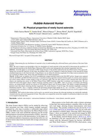
1. Astronomy
&
Astrophysics
A&A, 683, A122 (2024)
https://doi.org/10.1051/0004-6361/202346771
© The Authors 2024
Hubble Asteroid Hunter
III. Physical properties of newly found asteroids
Pablo García-Martín1
, Sandor Kruk2
, Marcel Popescu3,4
, Bruno Merín2
, Karl R. Stapelfeldt5
,
Robin W. Evans6
, Benoit Carry7
, and Ross Thomson8
1
Department of Theoretical Physics, Autonomous University of Madrid (UAM), Madrid 28049, Spain
e-mail: pablo.garciamartin@estudiante.uam.es
2
European Space Agency (ESA), European Space Astronomy Centre (ESAC), Camino Bajo del Castillo s/n, 28692 Villanueva de la
Cañada, Madrid, Spain
3
Astronomical Institute of the Romanian Academy, 5 Cutitul de Argint, 040557 Bucharest, Romania
4
University of Craiova, Str. A. I. Cuza nr. 13, 200585 Craiova, Romania
5
Jet Propulsion Laboratory, California Institute of Technology, Mail Stop 321-100, 4800 Oak Grove Drive, Pasadena, CA 91109, USA
6
Bastion Technologies, 17625 El Camino Real #330, Houston, TX 77058, USA
7
Université Côte d’Azur, Observatoire de la Côte d’Azur, CNRS, Laboratoire Lagrange, 06304 Nice, France
8
Google Cloud, 6425 Penn Ave, Pittsburgh, PA 15206, USA
Received 28 April 2023 / Accepted 22 December 2023
ABSTRACT
Context. Determining the size distribution of asteroids is key to understanding the collisional history and evolution of the inner Solar
System.
Aims. We aim to improve our knowledge of the size distribution of small asteroids in the main belt by determining the parallaxes of
newly detected asteroids in the Hubble Space Telescope (HST) archive and subsequently their absolute magnitudes and sizes.
Methods. Asteroids appear as curved trails in HST images because of the parallax induced by the fast orbital motion of the spacecraft.
Taking into account the trajectory of this latter, the parallax effect can be computed to obtain the distance to the asteroids by fitting
simulated trajectories to the observed trails. Using distance, we can obtain the absolute magnitude of an object and an estimation of its
size assuming an albedo value, along with some boundaries for its orbital parameters.
Results. In this work, we analyse a set of 632 serendipitously imaged asteroids found in the ESA HST archive. Images were captured
with the ACS/WFC and WFC3/UVIS instruments. A machine learning algorithm (trained with the results of a citizen science project)
was used to detect objects in these images as part of a previous study. Our raw data consist of 1031 asteroid trails from unknown
objects, not matching any entries in the Minor Planet Center (MPC) database using their coordinates and imaging time. We also
found 670 trails from known objects (objects featuring matching entries in the MPC). After an accuracy assessment and filtering
process, our analysed HST asteroid set consists of 454 unknown objects and 178 known objects. We obtain a sample dominated by
potential main belt objects featuring absolute magnitudes (H) mostly between 15 and 22 mag. The absolute magnitude cumulative
distribution logN(H > H0) ∝ α log(H0) confirms the previously reported slope change for 15 < H < 18, from α ≈ 0.56 to α ≈ 0.26,
maintained in our case down to absolute magnitudes of around H ≈ 20, and therefore expanding the previous result by approximately
two magnitudes.
Conclusions. HST archival observations can be used as an asteroid survey because the telescope pointings are statistically randomly
oriented in the sky and cover long periods of time. They allow us to expand the current best samples of astronomical objects at no extra
cost in regard to telescope time.
Key words. methods: data analysis – astronomical databases: miscellaneous – minor planets, asteroids: general
1. Introduction
The Solar System objects (SSOs) can be studied by observing
their movement over time, which requires multiple exposures
separated by a few days to produce a sufficiently large orbital
arc. If the SSOs have been reported to the Minor Planet Center
(MPC), which is the main worldwide repository for the receipt
and distribution of positional measurements of SSOs1
, precovery
in archival data can aid in orbit determination. In this paper, we
use a different method to characterise asteroids that relies on a set
of observations taken from low Earth orbit in large astronomical
archives.
1 https://www.zooniverse.org/projects/sandorkruk/
hubble-asteroid-hunter
Observatories in low Earth orbit confer a distinct advantage
in that their fast motion produces a parallax effect on the aster-
oid’s trail shape, allowing distance determination with fewer
observations. This parallax method was first devised by Evans
et al. (1998) and Evans & Stapelfeldt (2002) for use with aster-
oids identified in Hubble Space Telescope (HST) observations.
Figure 1 shows an example of an asteroid trail imaged by HST,
where the parallax effect is evident in the curvature of the trail.
In the Hubble Asteroid Hunter project2
(Kruk et al. 2022),
we identified 1,701 new asteroid trails in 19 yr of HST obser-
vations with the Advanced Camera for Surveys (ACS/WFC)
and Wide Field Camera 3 (WFC3/UVIS) observations, using
2 www.asteroidhunter.org
A122, page 1 of 10
Open Access article, published by EDP Sciences, under the terms of the Creative Commons Attribution License (https://creativecommons.org/licenses/by/4.0),
which permits unrestricted use, distribution, and reproduction in any medium, provided the original work is properly cited.
This article is published in open access under the Subscribe to Open model. Subscribe to A&A to support open access publication.

2. García-Martín, P., et al.: A&A, 683, A122 (2024)
Fig. 1. Example of asteroid trail imaged by HST in observation
idj554030 from WFC3/UVIS, taken on 5 Feb 2018. The trail spans
roughly 10 arcsec in RA and 8 arcsec in Dec.
a deep learning algorithm on Google Cloud, trained on vol-
unteer classifications from the Hubble Asteroid Hunter citizen
science project on the Zooniverse platform. 1031 (61%) of the
trails correspond to SSOs that we could not identify in the
MPC database. Considering how faint these asteroids are, many
of them are likely previously unidentified objects. The paral-
lax fitting method (Evans et al. 1998) is ideal for studying this
new sample of SSOs. By fitting the parallax for these trails,
we can determine the approximate orbital parameters of these
asteroids and derive their physical properties. Once we have
determined the distance to the asteroids, we can use their appar-
ent magnitudes to determine their intrinsic brightnesses and
sizes, assuming an average albedo value.
Studying faint asteroids is essential in order to better under-
stand their size distribution, which remains poorly understood
for small objects. The shape of the magnitude distribution curve,
as determined by Gladman et al. (2009), shows a shallower slope
for asteroids of smaller sizes down to H = 18 mag. This result
is crucial to our understanding of the evolution of the main belt
along with its collisional and dynamic depletion models (Bottke
et al. 2015).
Hubble Space Telescope observations taken over a long time
span can be effectively used as a randomly observed asteroid sur-
vey because the telescope’s pointing selections are statistically
random in the sky, and many observations are across the ecliptic
where the main asteroid belt is located.
This paper is structured as follows. In Sect. 2, we describe
the data that were used in this study. In Sect. 3, we outline
the parallax fitting method and examine its efficacy through
tests conducted on both simulated data and a sample of known
asteroids in the MPC database also identified by the Hubble
Asteroid Hunter citizen science project volunteers. Section 4
reports the results of the application of this method to previ-
ously unidentified asteroids, including the determination of their
orbital parameters and size distributions. In Sect. 5, we compare
our findings to those of previous studies. Finally, in Sect. 6 we
present our conclusions.
2. Data
The trails analysed in this work were obtained from the ESA
Hubble Space Telescope Archive for instruments ACS/WFC and
WFC3/UVIS. An object-detection machine learning algorithm
(trained with the results of a citizen science project) was used to
find asteroid trails (Kruk et al. 2022) and other objects of inter-
est such as gravitational lenses (Garvin et al. 2022) and satellite
trails (Kruk et al. 2023) in Hubble images from the archive
for both instruments. We used a total of 24 731 HST composite
images from ACS/WFC and 12 592 from WFC3/UVIS, each one
of them split into four quadrant cutouts to improve asteroid trail
detection efficiency. HST images from the archive were selected
based on the following criteria: no calibration images or ‘darks’;
exposure time greater than 100 seconds; FoV greater than 0.044◦
(avoiding subframes); and no grism spectral images, as their spe-
cial features could be confused with trails. We also removed any
image purposely targeting Solar System objects.
The volunteers of our citizen science project and also the
machine learning algorithm were trained to identify cosmic rays
to correctly distinguish their streaks from real asteroids. Never-
theless, the whole set of images featuring potential detections
was visually checked by the authors during the first part of this
project to avoid any artifact or spurious detection misidentified
as an asteroid.
Our data consist of 1031 asteroid trails from unknown
objects, not matching any entries in the MPC database based
on their coordinates and imaging time. We also found 670 trails
from known objects (objects featuring matching entries in the
MPC database), which proved very useful in testing and validat-
ing the method we propose in this work. For every case, a list of
right ascension (RA) and declination (Dec) coordinates forming
a trail is used along with the exposure starting and ending times.
Checking the identified trails for known objects was con-
ducted using a two-step process. The first step involved using
the average position and exposure time of each trail. We fed
this data to the SkyBoT service (Berthier et al. 2006, 2016),
performing a cone search with a 900 arcsec radius. This prelim-
inary step returned 22 748 possible candidates for our whole set.
During the second step, we filtered these candidates for precise
matches with the observed trails. For every image, ephemeris for
all its possible matches was retrieved from JPL Horizons service
(Giorgini et al. 1996) using the exposure time. We then anal-
ysed the approximate averaged distance between the observed
trail and those obtained from JPL Horizons (as seen from HST),
using a 3 arsec threshold for a positive match. The complete trail
processing pipeline applied during the first part of this project is
explained in full detail in Kruk et al. (2022).
3. Analysis methods
3.1. Parallax method
To obtain the distance to Earth of the unknown objects, we
present a method using the parallax-induced curvature of aster-
oid trails in HST images, following the work by Evans et al.
(1998) and Evans & Stapelfeldt (2002). Asteroid trails imaged
by HST present a very particular parallax induced by the space-
craft orbital motion around Earth while tracking a fixed target.
Being in a low Earth orbit, HST’s fast pace compared to its typi-
cal exposure times enables this unique effect for relatively close
objects in our Solar System. HST travels approximately one-third
of its orbit during a 30 min exposure (the average time for our
dataset); a stationary object situated at 2 AU from Earth (around
the main belt) could feature a parallax effect of up to ≈8 arcsec.
For every trail, HST orbital motion for the exposure time is
obtained from Jet Propulsion Laboratory (JPL) SPICE routines
(Acton 1996; Acton et al. 2018) along with Earth position with
respect to the Solar System Barycenter (SSB). Our code iter-
ates through different object distance solutions between 0.2 and
6.7 AU, obtaining predicted trails that are then compared to the
observed trail, looking for a best-fit solution. An upper distance
A122, page 2 of 10

3. García-Martín, P., et al.: A&A, 683, A122 (2024)
limit of 6.7 AU was chosen to potentially cover the Jupiter Tro-
jan asteroid population and also based on the non-curvature of
trails for objects located further away.
In addition to the parallax induced by the object’s distance
and HST–Earth trajectories, we also need to consider the object’s
motion around the Sun, which we refer to as the object’s intrinsic
rate of motion as observed in our images. The observed trail is
the linear combination of the parallax effect modelled by vector
P(∆, t) as a function of both observer distance (∆) and time (t),
and the object’s intrinsic rate of motion in RA and Dec: dα
dt and
dδ
dt , respectively.
From Evans et al. (1998), every point of the trail can then be
described as:
α − α0 = Pα(∆, t) +
dα
dt
· t
δ − δ0 = Pδ(∆, t) +
dδ
dt
· t,
(1)
where α0 and δ0 are the initial coordinates of the object; Pα and
Pδ are the components of vector P; dα
dt and dδ
dt are the intrinsic
rates of motion of the object, and t is the time of the exposure
being considered.
To obtain the observed object’s intrinsic rate of motion, we
use a rather straightforward method. The total span of the trail
in both RA and Dec coordinates must be equal to the aster-
oid motion rate plus the ‘deformation’ generated by the parallax
effect. Knowing the starting and ending points of the trail and
the standard deformation generated by the parallax at any given
distance, just one unique value of dα
dt and dδ
dt is possible for each
distance iteration.
The selected trail solution is the one featuring the lowest
error value χ2
as defined in Eq. (2), comparing the predicted
trails for 1300 different observer distance values (∆) and the
observed trail. We normalise χ2
using a 0.05 arcsec value, which
corresponds to the ACS/WFC pixel resolution (Ryon 2022).
The resolution achieved by WFC3/UVIS is 0.04 arcsec/pixel
(Dressel 2022), but we decided to use the worst ACS/WFC case
for our analysis to present a unified method for both instruments.
The χ2 expression is as follows:
χ2
=
1
n
X xcalc − xobs
0.05
2
, (2)
where n is the total number of existing points for the trail, xcalc
are the sky position values from the simulated trail being fitted,
and xobs are the observed trail sky position values.
During the first stage of this project (Kruk et al. 2022), the
trails were discretised by our extraction algorithm, finding the
maxima along each pixel column of the image cutout file. Tak-
ing the resolution of HST into account, this is approximately
one point every 0.04 arcsec for WCS3/UVIS and 0.05 arcsec
for ACS/WFC. The average number of points for a given trail
is approximately 300.
We cannot distinguish between distance solutions with a
mean fitting–residual difference of lower than the instrument res-
olution (considered to be one pixel, or 0.05′′
). Therefore, the
uncertainty Ur of our method is set by the two distance values
corresponding to χ2
+ 1 (as shown in Fig. 2).
Once we have a distance solution for a trail as seen from HST,
we obtain the distance to Earth and SSB using SPICE routines.
Given that all the analysed asteroids were serendipitously imaged
during a single HST observation, we cannot apply any standard
orbit approximation method. The object’s velocity component in
Fig. 2. Asteroid (511908) 2015 HU67. χ2
values showing a minimum
at the best-fit distance solution from Earth. The vertical line repre-
sents the actual distance for this object obtained from the JPL Horizons
ephemeris.
Fig. 3. Possible values of eccentricity (e, red) and inclination (i, blue) as
a function of semi-major axis (a) for asteroid (511908) 2015 HU67 cal-
culated using the parallax method. For every semi-major axis value, the
corresponding possible eccentricity and inclination solutions are shown
graphically.
the asteroid–Earth direction will always be missing and we can
only obtain the limits of its possible orbital parameters for semi-
major axis (a), eccentricity (e), and inclination (i).
Nevertheless, we can calculate some possible combinations
of these parameters supposing a bounded orbit. The object’s esti-
mated velocity and escape velocity are calculated from the obser-
vation (the object’s distance from the Sun can be obtained using
SPICE combined with the asteroid–Earth position obtained from
the parallax method) and 20 000 different velocity values for
the missing asteroid–Earth axis velocity component are iterated
using the escape velocity as a limit. We obtain a set of 20 000
possible orbital parameter combinations for each object, which
can be plotted as a function of semi-major axis as seen in Fig. 3.
We can also obtain minimum semi-major axis, eccentricity, and
inclination values for the object. Objects featuring estimated
velocities greater than their escape velocity are not considered
in our analysis and are expected to be cases where the method
will not be able to obtain a good result (see Sect. 3.2 for further
details on the filtering process).
A122, page 3 of 10

4. García-Martín, P., et al.: AA, 683, A122 (2024)
Fig. 4. Asteroid (511908) 2015 HU67. Observed trail from HST (blue)
vs best-fit distance solution using the parallax method (red). χ2
value
for this fitting is 0.13 (see Eq. (2)).
As an example of the parallax method, we show the results
for object (511908) 2015 HU67 identified in HST observation
idq27j020. This object is a relatively small asteroid from the mid-
dle main belt and features an apparent magnitude of 21.5 in the
V band. This trail was processed using our full code pipeline,
from trail coordinates to orbital parameter results. The trail fit
and χ2
minimum are shown in Figs. 4 and 2 respectively. The
graph featuring all possible inclination and eccentricity values
as a function of semi-major axis is shown in Fig. 3.
As a benchmark, we use the JPL Horizons ephemeris ser-
vice (Giorgini et al. 1996) to validate the parallax-obtained Earth
distance and orbital parameters for this known object. We show
this comparison in Table 1. Our parallax results show good
agreement with the values obtained from the database.
In some cases, the trail does not present enough curvature
to converge to a well-defined distance solution or to obtain a
reduced uncertainty interval allowing us to calculate a mean-
ingful absolute magnitude value. If the trail is not sufficiently
curved, our χ2
function will be too broad, implying a large
uncertainty Ur in the distance solutions. Trails lacking signifi-
cant curvature correspond to objects seen close to HST’s orbital
plane; that is, the induced parallax is close to the direction of
the asteroid’s intrinsic motion. The most curved trails are those
where the asteroid is seen at a large angle from HST’s orbital
plane, such that the induced parallax is becoming perpendicular
to the asteroid’s intrinsic motion.
An example of a trail not presenting a clear solution is object
(58250) 1993 QU1 featured in the HST image with observation
id j93y94010. Despite its high signal-to-noise ratio and good fit
(Fig. 5), the trail is too straight to yield an accurate distance solu-
tion and our method does not converge (Fig. 6). We can also
see in Fig. 6 that the trail fitting yields a large number of possi-
ble solutions inside the χ2
+ 1 threshold, as expected for straight
trails. The obtained Earth distance value is 6.695 AU (the actual
JPL Horizons Earth distance equals 2.382 AU). These cases were
filtered out from our sample as discussed in Sect. 3.2.
3.2. Assessing the accuracy of the method
To obtain a preliminary measure of the accuracy of our method,
we used 21 283 available known-asteroid ephemerides from the
JPL Horizons service (Giorgini et al. 1996) as a proof of concept
(POC) set. For every object, we input only the point coordinates
(RA and Dec) and time, as a real trail observed by HST, and
Table 1. Orbital parameters of (511908) 2015 HU67 from parallax
method vs JPL Horizons ephemeris data.
Feature Parallax results JPL Horizons
Earth dist. (AU) 1.610 1.607
SSB dist. (AU) 2.406 2.404
Phase ang. (deg) 17.941 18.137
Ecliptic lat. (deg) 1.824 1.820
e 0.162 e 0.275
i (deg) 4.178 i 4.909 4.733
a (AU) 1.897 a 2.585
Fig. 5. Object (58250) 1993 QU1. Example of a straight trail with no
parallax solution obtained.
Fig. 6. Object (58250) 1993 QU1. The method does not converge
because of the lack of curvature from the trail. The χ2
minimum is
obtained at the upper distance limit set in our code (≈6.7 AU). The
red line represents the actual Earth distance for this object from the JPL
Horizons ephemeris.
applied our method to calculate a distance solution. The obtained
distance from Earth was then compared with the distance value
provided by the JPL Horizons service. The global relative dis-
tance error (distance error divided by real object distance) results
for this POC set are centred around zero and can be seen in Fig. 7.
This confirms that our parallax method produces distance results
that are compatible with JPL Horizons database values. No fil-
ter or goodness-of-fit criteria were applied to the results of this
analysis or to the input data, which explains the long tails at both
ends of the error distribution. This result validates the accuracy
A122, page 4 of 10

5. García-Martín, P., et al.: AA, 683, A122 (2024)
Fig. 7. Relative distance error for JPL Horizons ephemeris distance vs
parallax-obtained distance for the proof-of-concept set (21 283 known
objects) using coordinates from JPL Horizons as simulated trails (RA,
Dec, and time). x-axis is distance error divided by actual distance. No
filtering or goodness of fit criteria were applied to this proof-of-concept
set, which explains the long tails at both ends of the distribution.
of our Python implementation of the method from Evans et al.
(1998), which was originally implemented in Fortran.
The next step is to evaluate our method in more detail and
precisely define its accuracy for distance predictions. To do so,
we used the 670 trails from known objects identified in the first
part of this project (Kruk et al. 2022). Of these 670 asteroids,
we selected the 452 featuring a permanent MPC designation
to reduce potential errors in their reference orbital parameters.
We ran the code using this group, which we name the known-
objects-validation set, and after examination we decided to apply
the following criteria to filter spurious distance results that could
contaminate our final population distribution. We excluded the
following objects:
– Objects presenting observed estimated velocities above
their escape velocity. No extra-solar objects were included in the
known objects set and the probability of finding one among our
results was deemed extremely unlikely.
– Objects above a 6.5 AU distance result or not featuring a
clear χ2
absolute minimum (Ur uncertainty equal to 0), for which
the method was not converging.
– Objects featuring an upper or lower distance uncertainty
Ur value equal to or greater than 35% of their actual distance.
We chose this value by analysing the relative error distribution
for the whole raw set (distance error divided by actual distance),
which represents one standard deviation (σ) for this distribution.
As mentioned above, these last two criteria are meant to filter out
trails that are too straight to yield a reliable parallax solution.
– Trails as non-monotonic functions (RA or Dec acting as
X–Y; see an example in Fig. 17 of Kruk et al. 2022). The
current version of our interpolation code is not adapted to han-
dling this kind of trail. We found less than five of these cases for
the considered analysis set, and so the impact versus effort ratio
was deemed too low to add this feature to our code. This option
should be considered for further work if larger data sets should
be analysed.
– Trails presenting background or close sources modifying
the extracted coordinates of the trail (see Kruk et al. (2022) for
Fig. 8. Distance to Earth relative error distribution (AU) for our known-
objects-validation set using HST trails (red) compared to the relative
error distribution for the synthetic trails validation set created using JPL
Horizons ephemerides for these same objects and time (green). x-axis
is distance error divided by actual distance.
the full trail coordinate extraction details) or other imaging arti-
facts such as trails slipping out of the cutouts. As mentioned
above, our code uses both the starting and ending points as
boundary conditions to obtain the object’s rates of motion along
with the image exposure time; it is especially sensitive to errors
originating from the incorrect definition of the two ends of a trail.
– Low-signal-to-noise-ratio trails, making coordinates diffi-
cult to obtain and trail limits difficult to measure.
We applied these criteria, keeping a total of 178 cases as
our final known-objects-validation set. We consider these cases
as a representative set to evaluate the accuracy of our parallax-
based method, having removed any external influence from HST
imaging or from our processing pipeline. This filtering process
features a very conservative approach for our selection crite-
ria, which led us to keeping about 40% of the initial processed
asteroids, optimising for detection quality over sample size.
The distance-to-Earth relative error distribution for this
known-objects-validation set is presented in Fig. 8 (distance
error divided by actual distance). This error was calculated by
comparing JPL Horizons Earth distance with the computed dis-
tance using the parallax method. We obtain a mean relative error
value centred at −1.2% and a standard deviation of σ = 10.5%.
This error distribution is presented to the reader as a global per-
formance indicator of our novel parallax method. It will not be
applied as an average error value to the results of this work.
The specific distance uncertainty is calculated for each object
as explained in Sect. 3.1.
To conduct a final verification of our method, we created a
synthetic validation set. Starting from the known objects val-
idation set, we obtained ‘synthetic’ trails from JPL Horizon
ephemerides for the same objects and exposure time as seen from
HST. We fed these trails to our code as real HST trails to obtain
a distance solution. In this case, the obtained mean relative error
value is −2.5% and σ = 7.5%. The comparison of both error dis-
tributions is shown in Fig. 8. Both error distributions are closely
overlapping and centred around zero, and therefore we consider
that any major influence from HST imaging or from our image
processing pipeline was correctly removed from our analysis.
As expected, we find a slight correlation between the actual
distance from the object to Earth, or its apparent magnitude, and
A122, page 5 of 10

6. García-Martín, P., et al.: AA, 683, A122 (2024)
Fig. 9. Scatter plot comparing the relative error on the distance to Earth
obtained from the parallax method vs the object’s actual Earth distance
and apparent magnitude.
Fig. 10. Absolute magnitude vs distance to Earth plot, comparing
our final known object validation set (red) with those removed dur-
ing the filtering process (grey). We can see a fairly random removal
process around both axes, without any effect depending on distance or
magnitude.
the distance error using the parallax method (see Fig. 9). In gen-
eral, distant (and probably faint) objects yield trails that are more
difficult to analyse because of the lower signal-to-noise ratios
and reduced parallax-induced curvature in the trails.
Another important aspect to assess when determining the
accuracy of our method is to make sure the filtering process
does not present any bias, removing fainter or smaller objects
and potentially reducing the number of outer main belt asteroids
in our observations. Figure 10 shows the initial sample of known
objects (452 asteroids) as a function of distance to Earth and
absolute magnitude (both parameters obtained from JPL Hori-
zons, considered as ground truth). Two different populations are
displayed in this figure: our final known object validation set
in red and the objects that were excluded during the filtering
process in grey. We see a fairly constant and random removal
process following both axes, without any systematic or selection
effects. As intended, our filtering process is mainly driven by
the characteristics of the trails, which are random, and not the
physical properties of the asteroids themselves.
3.3. Magnitude analysis
The apparent magnitudes of the trails were obtained in the pre-
vious part of this project (Kruk et al. 2022). We start from these
values to obtain the absolute magnitudes of the objects using the
distance solutions obtained with the parallax method.
Most of the unknown objects were serendipitously imaged by
HST in one single band, and no further information is available
about their colour or asteroid type. Although some of our detec-
tions come from the same HST observation set, we cannot link
the objects from one image to another, as we have no reliable
information about their orbital parameters. Before calculating
their absolute magnitude values, we transform the apparent mag-
nitude of each object in any given HST filter to a Johnson V
filter in order to apply a unified method to compare all of them.
We assume the asteroid spectra to be mostly the reflected spec-
trum from the Sun, except for their particular absorption features.
Therefore, the filter transformation value applied is the same
used for the spectrum of the Sun. Using the known objects set
as proof once again, we obtain a 0.18 mag average error for this
approximation.
Using the parallax-calculated distance and phase angle for
each object, we obtain its absolute magnitude using the equation
from Bowell et al. (1989):
H = V + 2.5 log10((1 − G)ϕ1 + Gϕ2) − 5 log10(∆ · r), (3)
where H is the object’s absolute magnitude, V is its apparent
magnitude in V, G is the photometric slope parameter, ∆ is the
object’s distance to Earth, and r is the object’s distance to the
Sun (both in AU). We used a G = 0.15 constant value for our
analysis. ϕ1 and ϕ2 parameters are functions of the phase angle
α of the object.
3.4. Size-estimation method
We use the absolute magnitude values (H) calculated in the
previous section to estimate the size of the analysed objects,
assuming them to be spherical and to feature a uniform surface
and therefore constant albedo. To do so, we applied the equation
from Harris Harris (1997). Even if albedo is known to change
from S-dominated to C-dominated taxonomy classes from the
inner to the outer belt (DeMeo Carry 2014), an average 0.15
albedo value was chosen for estimating the sizes of the objects.
This is an intermediate value representative of the typical range
(0.03 - 0.4) of asteroid compositional types (e.g. Mainzer et al.
2011; Popescu et al. 2018; Mahlke et al. 2022). To avoid any error
induced by this assumption, we used absolute magnitude (H) to
create the population size distribution graph discussed in Sect. 5
(Fig. 16). As an example, a H =19.5 object (around the median
value for our unknown objects set) will feature a diameter of
≈700 m if supposing a 0.05 albedo and ≈330 m if we suppose a
0.25 albedo.
4. Results
We applied the methods described to the set of 1031 unknown
Solar System Objects from Kruk et al. (2022). The strict filtering
criteria we present in Sect. 3.2 yield a total of 454 objects. This
filtered set is ≈44% of the original number, matching the yield
obtained for the known-objects-validation set after cleansing.
As stated in the previous sections, we prioritised high preci-
sion over a large population of objects. The majority of the input
objects are purposely excluded during these filtering processes
to maximise accuracy.
A122, page 6 of 10

7. García-Martín, P., et al.: AA, 683, A122 (2024)
Fig. 11. Distance to SSB for known (red) and unknown (blue) objects.
Unknown object values were obtained from the parallax method, known
object values from the JPL Horizons database.
Fig. 12. Distance to Earth for known (red) and unknown (blue) objects.
Unknown object values were obtained from the parallax method, known
object values from the JPL Horizons database.
For the histograms of this section, data for known objects are
extracted directly from the JPL Horizons database, which is con-
sidered as a baseline and therefore do not feature any uncertainty
bars in any of the presented graphs. The uncertainty bars for the
histograms of unknown objects were obtained using bootstrap-
ping (Efron 1982), randomly resampling the existing population
1000 times and calculating the standard deviation for each bin.
4.1. Object distance
We obtained the distance to Earth and the distance to the Solar
System Barycenter (SSB) for the 454 unknown objects. Results
can be seen in Figs. 11 and 12. Both distance distributions fea-
ture a close overlap for known and unknown objects, centred
around the main belt in both cases. There is a small bump for
unknown objects at less than 1 AU from Earth, representing
close objects spotted by HST. Given the limited nature of our
calculated orbital parameters, we cannot obtain a real perihelion
value and therefore cannot assess whether or not they could be
near-Earth objects (NEOs), as we argue in Sect. 5.
Fig. 13. Absolute magnitude (H) for known (red) and unknown objects
(blue) from JPL Horizons database and calculated using the distance
obtained with the parallax method, respectively. The upper axis shows
the approximate object size using a 0.15 albedo value.
Fig. 14. Size distribution for unknown objects (using a 0.15 albedo
value).
4.2. Magnitude and size distributions
Despite having obtained a very close distance distribution for
known and unknown objects (either to Earth or SSB), if we take a
look at the absolute magnitude results displayed in Fig. 13 we can
see that the unknown objects population is dominated by fainter
objects centred around H = 19–20 magnitude. Both results indi-
cate that we are mostly imaging small (1 km) main belt objects
not easily accessible using ground-based asteroid surveys.
The size distribution for the unknown objects (assuming an
average albedo of 0.15 for all objects) is presented in Fig. 14. A
significant portion of them are below 1 km in size.
5. Discussion
5.1. Size and absolute magnitude population distributions
A scatter plot presenting size as a function of distance from
Earth is shown in Fig. 15. As we can see, the lower size limit
of the detected unknown objects increases with distance from
A122, page 7 of 10

8. García-Martín, P., et al.: AA, 683, A122 (2024)
Fig. 15. Size vs Earth distance for the known-objects-validation set
(grey) and the unknown objects set (green, using a 0.15 albedo value
to estimate size). For clarity, the average size and distance uncertainties
are displayed next to the main population area as a black cross.
Earth, as expected for a flux-limited survey. The unique capabil-
ities of HST allow us to detect unknown objects up to distances
of around 3 AU from Earth (with the main population centred
around 2 AU) and below a 1 km estimated diameter. We find that
our unknown objects population is mainly composed of small
main belt asteroids (1 km size).
Assuming that the size distribution is the same everywhere
in the asteroid belt and despite the fact that our total dataset
(unknown + known objects) does not represent a dedicated or
observationally unbiased asteroid survey, we can use our HST
set as a random asteroid population sample given the large time
span covered by our HST archival analysis (19 yr) and the sta-
tistically random HST pointing locations (Kruk et al. 2022). As
shown in Figs. 11 and 15, most of our objects are found in the
main belt. If we take a closer look at Fig. 15, we can clearly see
the cutoff generated by the lower part of the scatter plot, which
represents the observational limit of HST for a given distance.
For a distance of 2.5 AU from Earth, which is roughly the end
of the outer main belt, our size detection limit is 0.5 km, equiv-
alent to H ≈ 19.5 using a 0.15 albedo. We assume our dataset to
be complete up to this magnitude value regarding the main belt
asteroid population.
The new population model we present is based on absolute
magnitude (H) and is depicted in Fig. 16. We present the entire
HST set (unknown and known asteroids), featuring 632 objects.
We identify two different approximate values for the slope of
our cumulative distribution function: log N(H H0) ∝ (0.56 ±
0.12) log(H0) for H values between 12 and 15, and log N(H
H0) ∝ (0.26 ± 0.06) log(H0) for H values between 15 and 20.
Above H ≈ 19–20, our dataset reaches its detection limit.
The values we obtained can be compared with the results
from the Sub-Kilometer Asteroid Diameter Survey (SKADS;
Gladman et al. 2009). This dedicated and debiased survey for
main belt small objects yields a slope of α = 0.3 ± 0.02 for H
values between 15 and 18, in agreement with the value obtained
in our analysis. The slight difference could be explained by our
HST dataset bias, its incompleteness, or the different filters used
in the two analyses. The steeper slope change for the H 15
regime is also described in this work, with a reported value of
Fig. 16. Absolute magnitude cumulative size distribution for our HST
dataset. The black lines and numerical values represent the calculated
approximate equivalent slopes α for log N(H H0) ∝ α log(H0).
α = 0.5, which is very close to the value found for the HST aster-
oids set (α = 0.56). Our work shows that the α = 0.3 slope value
between 15 and 18 H remains consistent up to H ≈ 19–20 mag.
For reference, H ≈ 15 corresponds to a size of 3 km for an albedo
of 0.15.
Other previous works found results compatible with our sur-
vey. Using observations from WISE/NEOWISE in the thermal
infrared, Masiero et al. (2011) found a size distribution slope
for main belt objects in good agreement with that found by
Gladman et al. (2009), which is considered as the benchmark
for our work. Still in the infrared and using data from Spitzer,
Ryan et al. (2015) found a slightly shallower population distribu-
tion slope with a ‘kink’ or inflection point around a diameter of
8 km, corresponding roughly to H ≈ 13 using a 0.15 albedo. In
our case, we do not have enough observations around this magni-
tude value to confirm this feature. Heinze et al. (2019) performed
main belt observations from the Blanco Telescope at Cerro
Tololo Inter-American Observatory, reporting a non-constant
population power-law slope. In this latter work, the apparent
R-band population distribution shows a transition around R =
19–20, with a shallower slope for fainter magnitudes, which is in
good agreement with our benchmark (Gladman et al. 2009).This
shallower slope is maintained up to two fainter magnitudes than
Gladman et al. (2009), which reinforces the results from our
work showing a constant slope maintained up to H ≈ 19-20 mag.
Maeda et al. (2021) found a similar shape for both ‘C-like’ and
‘S-like’ size population distributions featuring main belt aster-
oids between 0.4 and 5 km in size (roughly H ≈ 20 and H ≈ 14
using a 0.15 albedo). This similarity between the two types of
asteroids supports the average nature of our population distri-
bution, not being able to reliably distinguish asteroid classes in
our unknown objects HST set. These latter authors also report
an inflection point in the slope of the absolute magnitude popu-
lation distribution that is located at around 1.7 mag fainter than
the inflection point found in the present study. Slope values are
α = 0.55 and α = 0.23; that is, slightly shallower for the fainter
end.
5.2. Potential comets
An interesting possibility suggested by our findings is the exis-
tence of objects with orbits consistent to those of comets. To
A122, page 8 of 10

9. García-Martín, P., et al.: AA, 683, A122 (2024)
Table 2. Two examples of potential comets found in our dataset and
their calculated approximate orbital parameters.
Image j8n218010 j90i02010
Earth dist. (AU) 0.55 +0.02 −0.03 2.91 +0.10 −0.10
SSB dist. (AU) 1.52 +0.01 −0.03 3.10 +0.10 −0.10
H 22.15 +0.16 −0.08 18.35 +0.14 −0.14
TJ (I min) 1.69 1.07
e 0.91 e 0.52 e
i (deg) 17.35 i 17.63 82.08 i 99.79
a (AU) 15.59 a 6.44 a
Min. perihelion (AU) 1.37 3.08
Fig. 17. Two examples of potential comets found in our dataset.
Left images correspond to j8n218010 and right images to j90i02010.
The upper row represents the original trail cutouts and the lower
row the identified trail centerline and trail extraction lateral limits
(Kruk et al. 2022).
help us find possible candidates, we calculated the Tisserand’s
parameter (Tisserand 1889) with respect to Jupiter (TJ) as seen
in Eq. (4), using the object’s minimum inclination, eccentricity,
and semi-major axis values.
TJ =
aJ
a
+ 2
s
(1 − e2)a
aJ
· cos(i), (4)
where aJ is Jupiter’s semi-major axis, a is the object’s minimum
semi-major axis, e is the object’s minimum eccentricity, and i is
the object’s minimum inclination.
We find 45 objects of interest featuring TJ 3. This repre-
sents ≈10% of the total 454 analysed objects. Two examples are
displayed in Table 2 and Fig. 17. All the 45 candidates present
apparent magnitudes of between 22.2 and 25.1 mag in the given
filters used by HST for each observation, making them realistic
candidate new objects featuring comet orbits.
We note that TJ parameter provides a first indication of
a cometary orbit. The Jupiter family comets are characterised
by 2 ≤ TJ ≥ 3, while for the long-period comets, TJ 2. An
enhanced criterion to identify cometary orbits is provided by
Tancredi (2014); it takes into account the orbital parameters
and the minimum orbital intersection distance, and discards the
objects in mean motion resonances.
5.3. Potential near-Earth objects
Near-Earth objects are also a relevant class of objects, and merit
a more detailed analysis to find potential candidates in our
dataset. We define NEOs as objects featuring a perihelion of
1.3 AU (Bottke et al. 2002). Considering that we only have
lower limits for eccentricity and semi-major axis, the calcu-
lated perihelion and aphelion values are also approximations and
should only be used as an indicator of potential objects belong-
ing to this family (shown in the lower-left corner of Fig. 15). We
find 74 potential NEO candidates. The apparent magnitudes in
this case span from 20.4 to 25.1 in the given filter used by HST
to take the image.
Among our NEO set, we find ∼34% Amors, ∼41% Apollos,
and ∼12% Atens. These values are close to but not coincident
with those from Granvik et al. (2018), who present a popu-
lation distribution for NEOs in the range of 17 H 25,
featuring a relative share of 39.4% Amors, 54.4% Apollos, and
3.5% Atens. In our case, our analysis is limited by the approx-
imate nature of the orbital parameters and HST observational
bias for NEOs. Our dataset does not represent a complete popu-
lation model for this kind of object (which is beyond the scope
of this work) but a random sample of observations from HST
archival data.
5.4. Further work
Absolute magnitude distributions can be used to estimate the
size distribution after a careful estimation of the albedo val-
ues, such as in the study conducted by Ivezić et al. (2001)
using commissioning data from SDSS and including colour
information.
We are also currently analysing the light curves from all the
detected asteroids (known and unknown objects). This analy-
sis should lead to a better characterisation of the properties of
small objects, which are important in order to fully understand
the collisional and dynamical main belt evolution (Bottke et al.
2015). The raw light curves from this project require specialised
processing in order to take into account the parallax effect and
correctly project time versus brightness variation.
Beyond the discovery and physical characterisation of small
asteroids in the HST archive, all three of the papers from the
Hubble Asteroid Hunter project illustrate how the training of
deep learning neural networks to identify objects in images –
or other features in science data archives – using labels produced
by large citizen science projects could be used to automatically
tag objects or phenomena in scientific datasets and assist data
analysts in the subsequent identification of such types of objects
or phenomena, greatly enlarging the scientific potential of such
datasets. Encouraged by these prolific citizen science projects,
ESA has launched another two similar citizen science projects
(Rosetta Zoo3
and GaiaVari4
) where volunteers are asked to clas-
sify moving features on the surface of the comet 67P as observed
by the Rosetta mission or classify different types of variable stars
in the Gaia catalogue. The results of these projects will also be
used to train deep neural networks that will allow the identifica-
tion and classification of such features in future datasets (from
similar or the same missions) reliably and automatically. In the
particular case of the asteroids, serendipitous observations made
3 https://www.zooniverse.org/projects/ellenjj/
rosetta-zoo/
4 https://www.zooniverse.org/projects/gaia-zooniverse/
gaia-vari
A122, page 9 of 10

10. García-Martín, P., et al.: AA, 683, A122 (2024)
by JWST will probably become a substantial source of new aster-
oid detections, as demonstrated recently by Müller et al. (2023).
The ESA Euclid mission will also enable many new object dis-
coveries in the years to come thanks to its large field of view
combined with its spatial resolution (Carry 2018; Pöntinen et al.
2020). Unfortunately, in both JWST and Euclid cases, their orbits
around L2 are not suited to induce parallax in the same way
as HST.
6. Conclusions
We analysed the physical properties of a set of 632 serendipi-
tously imaged asteroids from the HST archive. These asteroids
were found using a combination of a citizen science project
and a machine learning algorithm as part of a previous study
(Kruk et al. 2022). To obtain asteroid distances from just one
observation, we applied a proven method based on the parallax
effect generated by HST’s low Earth orbit (Evans et al. 1998).
Approximately 40% of the raw objects found in the archive
yield meaningful distance results using this method. We used
these distance results to compute the absolute magnitude and
approximate size of the asteroids.
Our results indicate a set dominated by main belt objects fea-
turing sizes of below 10 km and absolute magnitudes (H) mostly
between 15 and 22. The unknown objects set (454 objects) is
bounded below 1 km size and between 17 and 22 for H. The
absolute magnitude cumulative distribution confirms the previ-
ously reported slope change at H = 15 for main belt objects
(Gladman et al. 2009), from α ≈ 0.56 to α ≈ 0.26, with this lat-
ter slope being maintained up to absolute magnitudes of around
H ≈ 20 in our case.
One of the advantages of applying machine learning to
find Solar System objects in complete astronomical archives is
the large number of potential results obtained. This allows us
to apply purposely strict filtering conditions to improve accu-
racy and still keep a large enough sample to obtain statistically
meaningful results.
Adding automatic SSO detection pipelines to deep but FoV-
limited telescopes could generate important contributions to the
population of small SSOs and to our understanding of the early
stages and evolution of the Solar System. In our case, the anal-
ysis of archival data spanning 19 yr limits the possibilities of
any object follow up for interesting cases such as potential
NEOs or comets. This drawback can be avoided using real-time
processing pipelines.
We have contacted the IAU Minor Planet Center to submit
the full identifications set (known and unknown objects) for the
whole Hubble Asteroid Hunter Project (Kruk et al. 2022).
Acknowledgements. We thank the anonymous referee for the helpful comments
and suggestions that led to the improvement of this manuscript. We acknowledge
support from ESA through the Science Faculty – Funding reference ESA-SCI-
SC-LE-154. This work was possible thanks to the Google Cloud Research
Credits Program. The work of M.P. was supported by a grant of the Romanian
National Authority for Scientific Research – UEFISCDI, project number PN-III-
P2-2.1-PED-2021-3625. We want to specially thank the STScI helpdesk for their
quick responses and useful advice. This publication uses data generated via the
https://www.zooniverse.org/ platform, development of which is funded by
generous support, including a Global Impact Award from Google, and by a grant
from the Alfred P. Sloan Foundation. This work has made extensive use of data
from HST mission, hosted by the European Space Agency at the eHST archive, at
ESAC (https://www.cosmos.esa.int/hst), thanks to a partnership with the
Space Telescope Science Institute, in Baltimore, USA (https://www.stsci.
edu/) and with the Canadian Astronomical Data Centre, in Victoria, Canada
(https://www.cadc-ccda.hia-iha.nrc-cnrc.gc.ca/).
References
Acton, C. H. 1996, Planet. Space Sci., 44, 65
Acton, C., Bachman, N., Semenov, B., Wright, E. 2018, Planet. Space Sci.,
150, 9
Berthier, J., Vachier, F., Thuillot, W., et al. 2006, ASP Conf. Ser., 351, 367
Berthier, J., Carry, B., Vachier, F., Eggl, S., Santerne, A. 2016, MNRAS, 458,
3394
Bottke, W. F., Brož, M., O’Brien, D. P., et al. 2015, in Asteroids IV, 701
Bottke, W. F., Morbidelli, A., Jedicke, R., et al. 2002, Icarus, 156, 399
Bowell, E., Hapke, B., Domingue, D., et al. 1989, in Asteroids II, 524
Carry, B. 2018, AA, 609, A113
DeMeo, F. E., Carry, B. 2014, Nature, 505, 629
Dressel, L. 2022, in WFC3 Instrument Handbook for Cycle 30 v. 14 (Baltimore:
STScI)
Efron, B. 1982, CBMS-NSF Regional Conference Series in Applied Mathemat-
ics (Philadelphia: Society for Industrial and Applied Mathematics (SIAM))
Evans, R. W., Stapelfeldt, K. R. 2002, in ESA SP, 500, 509
Evans, R. W., Stapelfeldt, K. R., Peters, D. P., et al. 1998, Icarus, 131, 261
Garvin, E. O., Kruk, S., Cornen, C., et al. 2022, AA, 667, A141
Giorgini, J. D., Yeomans, D. K., Chamberlin, A. B., et al. 1996, in AAS/Division
for Planetary Sciences Meeting Abstracts, #28, 25.04
Gladman, B. J., Davis, D. R., Neese, C., et al. 2009, Icarus, 202, 104
Granvik, M., Morbidelli, A., Jedicke, R., et al. 2018, Icarus, 312, 181
Harris, A. W., Harris, A. W. 1997, Icarus, 126, 450
Heinze, A. N., Trollo, J., Metchev, S. 2019, AJ, 158, 232
Ivezić, Ž., Tabachnik, S., Rafikov, R., et al. 2001, AJ, 122, 2749
Kruk, S., García Martín, P., Popescu, M., et al. 2022, AA, 661, A85
Kruk, S., García-Martín, P., Popescu, M., et al. 2023, Nat. Astron., 7, 262
Maeda, N., Terai, T., Ohtsuki, K., et al. 2021, AJ, 162, 280
Mahlke, M., Carry, B., Mattei, P. A. 2022, AA, 665, A26
Mainzer, A., Grav, T., Masiero, J., et al. 2011, ApJ, 741, 90
Masiero, J. R., Mainzer, A. K., Grav, T., et al. 2011, ApJ, 741, 68
Müller, T. G., Micheli, M., Santana-Ros, T., et al. 2023, AA, 670, A53
Pöntinen, M., Granvik, M., Nucita, A. A., et al. 2020, AA, 644, A35
Popescu, M., Licandro, J., Carvano, J. M., et al. 2018, AA, 617, A12
Ryan, E. L., Mizuno, D. R., Shenoy, S. S., et al. 2015, AA, 578, A42
Ryon, J. E. 2022, in ACS Instrument Handbook for Cycle 30 v. 21.0 (Baltimore:
STScI)
Tancredi, G. 2014, Icarus, 234, 66
Tisserand, F. 1889, Bull. Astron. Ser. I, 6, 241
A122, page 10 of 10